Gmaps Documentation Release 0.8.3-dev - Pascal Bugnion - Read the Docs
←
→
Page content transcription
If your browser does not render page correctly, please read the page content below
gmaps Documentation
        Release 0.8.3-dev

         Pascal Bugnion

                Jan 13, 2019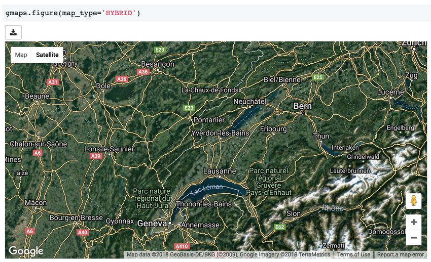
Contents

1   Installation                                                                                                                                                                                            1
    1.1 Installing jupyter-gmaps with conda . .                         .   .   .   .   .   .   .   .   .   .   .   .   .   .   .   .   .   .   .   .   .   .   .   .   .   .   .   .   .   .   .   .   .   1
    1.2 Installing jupyter-gmaps with pip . . .                         .   .   .   .   .   .   .   .   .   .   .   .   .   .   .   .   .   .   .   .   .   .   .   .   .   .   .   .   .   .   .   .   .   1
    1.3 Installing jupyter-gmaps for JupyterLab                         .   .   .   .   .   .   .   .   .   .   .   .   .   .   .   .   .   .   .   .   .   .   .   .   .   .   .   .   .   .   .   .   .   1
    1.4 Development version . . . . . . . . . .                         .   .   .   .   .   .   .   .   .   .   .   .   .   .   .   .   .   .   .   .   .   .   .   .   .   .   .   .   .   .   .   .   .   2
    1.5 Source code . . . . . . . . . . . . . .                         .   .   .   .   .   .   .   .   .   .   .   .   .   .   .   .   .   .   .   .   .   .   .   .   .   .   .   .   .   .   .   .   .   2

2   Authentication                                                                                                                                                                                          3

3   Getting started                                                                                                                                                                                          5
    3.1 Basic concepts . . . . . . . . . . . . . . .                            .   .   .   .   .   .   .   .   .   .   .   .   .   .   .   .   .   .   .   .   .   .   .   .   .   .   .   .   .   .   .    6
    3.2 Base maps . . . . . . . . . . . . . . . . .                             .   .   .   .   .   .   .   .   .   .   .   .   .   .   .   .   .   .   .   .   .   .   .   .   .   .   .   .   .   .   .    9
    3.3 Customising map width, height and layout                                .   .   .   .   .   .   .   .   .   .   .   .   .   .   .   .   .   .   .   .   .   .   .   .   .   .   .   .   .   .   .   11
    3.4 Heatmaps . . . . . . . . . . . . . . . . . .                            .   .   .   .   .   .   .   .   .   .   .   .   .   .   .   .   .   .   .   .   .   .   .   .   .   .   .   .   .   .   .   12
    3.5 Weighted heatmaps . . . . . . . . . . . . .                             .   .   .   .   .   .   .   .   .   .   .   .   .   .   .   .   .   .   .   .   .   .   .   .   .   .   .   .   .   .   .   15
    3.6 Markers and symbols . . . . . . . . . . . .                             .   .   .   .   .   .   .   .   .   .   .   .   .   .   .   .   .   .   .   .   .   .   .   .   .   .   .   .   .   .   .   16
    3.7 GeoJSON layer . . . . . . . . . . . . . . .                             .   .   .   .   .   .   .   .   .   .   .   .   .   .   .   .   .   .   .   .   .   .   .   .   .   .   .   .   .   .   .   20
    3.8 Drawing markers, lines and polygons . . .                               .   .   .   .   .   .   .   .   .   .   .   .   .   .   .   .   .   .   .   .   .   .   .   .   .   .   .   .   .   .   .   24
    3.9 Directions layer . . . . . . . . . . . . . .                            .   .   .   .   .   .   .   .   .   .   .   .   .   .   .   .   .   .   .   .   .   .   .   .   .   .   .   .   .   .   .   26
    3.10 Bicycling, transit and traffic layers . . . . .                        .   .   .   .   .   .   .   .   .   .   .   .   .   .   .   .   .   .   .   .   .   .   .   .   .   .   .   .   .   .   .   29

4   Building applications with jupyter-gmaps                                                                                                                                                                33
    4.1 Reacting to user actions on the map . . . . . . . . . . . . . . . . . . . . . . . . . . . . . . . . . . .                                                                                           33
    4.2 Updating a heatmap in response to other widgets . . . . . . . . . . . . . . . . . . . . . . . . . . . .                                                                                             36
    4.3 Updating symbols in response to other widgets . . . . . . . . . . . . . . . . . . . . . . . . . . . . .                                                                                             38

5   Exporting maps                                                                                                                                                                                          43
    5.1 Exporting to PNG . . . . . . . . . . . . . . . . . . . . . . . . . . . . . . . . . . . . . . . . . . . .                                                                                            43
    5.2 Exporting to HTML . . . . . . . . . . . . . . . . . . . . . . . . . . . . . . . . . . . . . . . . . . .                                                                                             43

6   API documentation                                                                                                                                                                                       45
    6.1 Figures and layers . .      .   .   .   .   .   .   .   .   .   .   .   .   .   .   .   .   .   .   .   .   .   .   .   .   .   .   .   .   .   .   .   .   .   .   .   .   .   .   .   .   .   .   45
    6.2 Utility functions . . .     .   .   .   .   .   .   .   .   .   .   .   .   .   .   .   .   .   .   .   .   .   .   .   .   .   .   .   .   .   .   .   .   .   .   .   .   .   .   .   .   .   .   55
    6.3 Low level widgets . .       .   .   .   .   .   .   .   .   .   .   .   .   .   .   .   .   .   .   .   .   .   .   .   .   .   .   .   .   .   .   .   .   .   .   .   .   .   .   .   .   .   .   56
    6.4 Datasets . . . . . . . .    .   .   .   .   .   .   .   .   .   .   .   .   .   .   .   .   .   .   .   .   .   .   .   .   .   .   .   .   .   .   .   .   .   .   .   .   .   .   .   .   .   .   68
    6.5 GeoJSON geometries          .   .   .   .   .   .   .   .   .   .   .   .   .   .   .   .   .   .   .   .   .   .   .   .   .   .   .   .   .   .   .   .   .   .   .   .   .   .   .   .   .   .   69
    6.6 Traitlets . . . . . . . .   .   .   .   .   .   .   .   .   .   .   .   .   .   .   .   .   .   .   .   .   .   .   .   .   .   .   .   .   .   .   .   .   .   .   .   .   .   .   .   .   .   .   69

                                                                                                                                                                                                             i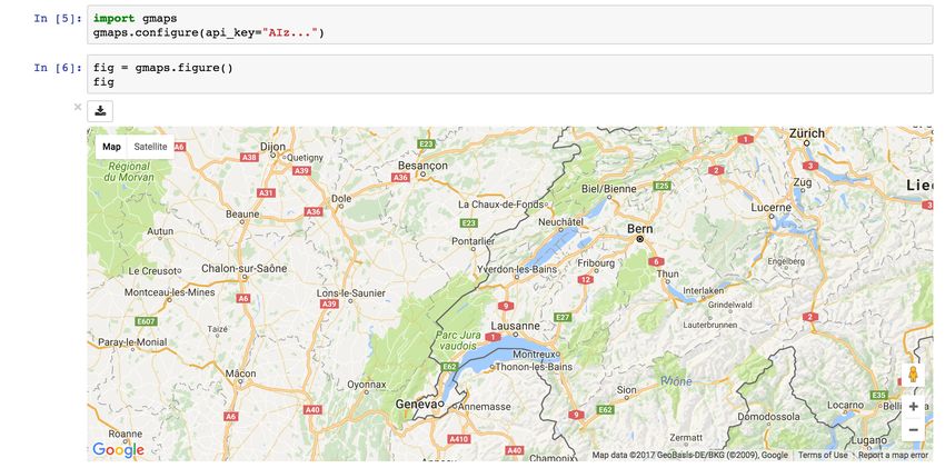
7    Contributing to jupyter-gmaps                                                                                                                                                          71
     7.1 Contributing . . . . . . . . . . . . . . . . . . . . . . . . . . . . . . . . . . . . . . . . . . . . . . .                                                                         71
     7.2 How to release jupyter-gmaps . . . . . . . . . . . . . . . . . . . . . . . . . . . . . . . . . . . . . .                                                                           72

8    Release notes                                                                                                                                                                          73
     8.1 Version 0.8.2 . . . . . . . . . . . . .    .   .   .   .   .   .   .   .   .   .   .   .   .   .   .   .   .   .   .   .   .   .   .   .   .   .   .   .   .   .   .   .   .   .   73
     8.2 Version 0.8.1 - 26th September 2018        .   .   .   .   .   .   .   .   .   .   .   .   .   .   .   .   .   .   .   .   .   .   .   .   .   .   .   .   .   .   .   .   .   .   73
     8.3 Version 0.8.0 - 22nd April 2018 . . .      .   .   .   .   .   .   .   .   .   .   .   .   .   .   .   .   .   .   .   .   .   .   .   .   .   .   .   .   .   .   .   .   .   .   73
     8.4 Version 0.7.4 - 5th April 2018 . . . .     .   .   .   .   .   .   .   .   .   .   .   .   .   .   .   .   .   .   .   .   .   .   .   .   .   .   .   .   .   .   .   .   .   .   74
     8.5 Version 0.7.3 - 11th March 2018 . . .      .   .   .   .   .   .   .   .   .   .   .   .   .   .   .   .   .   .   .   .   .   .   .   .   .   .   .   .   .   .   .   .   .   .   74
     8.6 Version 0.7.2 - 16th February 2018 .       .   .   .   .   .   .   .   .   .   .   .   .   .   .   .   .   .   .   .   .   .   .   .   .   .   .   .   .   .   .   .   .   .   .   74
     8.7 Version 0.7.1 - 10th February 2018 .       .   .   .   .   .   .   .   .   .   .   .   .   .   .   .   .   .   .   .   .   .   .   .   .   .   .   .   .   .   .   .   .   .   .   74
     8.8 Version 0.7.0 - 11th November 2017 .       .   .   .   .   .   .   .   .   .   .   .   .   .   .   .   .   .   .   .   .   .   .   .   .   .   .   .   .   .   .   .   .   .   .   74
     8.9 Version 0.6.2 - 30th October 2017 . .      .   .   .   .   .   .   .   .   .   .   .   .   .   .   .   .   .   .   .   .   .   .   .   .   .   .   .   .   .   .   .   .   .   .   75
     8.10 Version 0.6.1 - 1st September 2017 .      .   .   .   .   .   .   .   .   .   .   .   .   .   .   .   .   .   .   .   .   .   .   .   .   .   .   .   .   .   .   .   .   .   .   75
     8.11 Version 0.6.0 - 26th August 2017 . .      .   .   .   .   .   .   .   .   .   .   .   .   .   .   .   .   .   .   .   .   .   .   .   .   .   .   .   .   .   .   .   .   .   .   75
     8.12 Version 0.5.4 - 15th July 2017 . . . .    .   .   .   .   .   .   .   .   .   .   .   .   .   .   .   .   .   .   .   .   .   .   .   .   .   .   .   .   .   .   .   .   .   .   75
     8.13 Version 0.5.3 - 8th July 2017 . . . . .   .   .   .   .   .   .   .   .   .   .   .   .   .   .   .   .   .   .   .   .   .   .   .   .   .   .   .   .   .   .   .   .   .   .   75
     8.14 Version 0.5.2 - 25th June 2017 . . . .    .   .   .   .   .   .   .   .   .   .   .   .   .   .   .   .   .   .   .   .   .   .   .   .   .   .   .   .   .   .   .   .   .   .   76
     8.15 Version 0.5.1 - 3rd June 2017 . . . .     .   .   .   .   .   .   .   .   .   .   .   .   .   .   .   .   .   .   .   .   .   .   .   .   .   .   .   .   .   .   .   .   .   .   76
     8.16 Version 0.5.0 - 8th May 2017 . . . .      .   .   .   .   .   .   .   .   .   .   .   .   .   .   .   .   .   .   .   .   .   .   .   .   .   .   .   .   .   .   .   .   .   .   76
     8.17 Version 0.4.1 - 14th March 2017 . . .     .   .   .   .   .   .   .   .   .   .   .   .   .   .   .   .   .   .   .   .   .   .   .   .   .   .   .   .   .   .   .   .   .   .   76
     8.18 Version 0.4.0 - 28th January 2017 . .     .   .   .   .   .   .   .   .   .   .   .   .   .   .   .   .   .   .   .   .   .   .   .   .   .   .   .   .   .   .   .   .   .   .   77
     8.19 Version 0.3.6 - 28th December 2016 .      .   .   .   .   .   .   .   .   .   .   .   .   .   .   .   .   .   .   .   .   .   .   .   .   .   .   .   .   .   .   .   .   .   .   77
     8.20 Version 0.3.5 - 8th October 2016 . . .    .   .   .   .   .   .   .   .   .   .   .   .   .   .   .   .   .   .   .   .   .   .   .   .   .   .   .   .   .   .   .   .   .   .   77
     8.21 Version 0.3.4 - 26th September 2016       .   .   .   .   .   .   .   .   .   .   .   .   .   .   .   .   .   .   .   .   .   .   .   .   .   .   .   .   .   .   .   .   .   .   77
     8.22 Version 0.3.3 - 7th September 2016 .      .   .   .   .   .   .   .   .   .   .   .   .   .   .   .   .   .   .   .   .   .   .   .   .   .   .   .   .   .   .   .   .   .   .   77
     8.23 Version 0.3.2 - 30th July 2016 . . . .    .   .   .   .   .   .   .   .   .   .   .   .   .   .   .   .   .   .   .   .   .   .   .   .   .   .   .   .   .   .   .   .   .   .   77
     8.24 Version 0.3.1 - 30th July 2016 . . . .    .   .   .   .   .   .   .   .   .   .   .   .   .   .   .   .   .   .   .   .   .   .   .   .   .   .   .   .   .   .   .   .   .   .   77
     8.25 Version 0.3.0 - 14th June 2016 . . . .    .   .   .   .   .   .   .   .   .   .   .   .   .   .   .   .   .   .   .   .   .   .   .   .   .   .   .   .   .   .   .   .   .   .   78
     8.26 Version 0.2.2 - 26th March 2016 . . .     .   .   .   .   .   .   .   .   .   .   .   .   .   .   .   .   .   .   .   .   .   .   .   .   .   .   .   .   .   .   .   .   .   .   78
     8.27 Version 0.2.1 - 26th March 2016 . . .     .   .   .   .   .   .   .   .   .   .   .   .   .   .   .   .   .   .   .   .   .   .   .   .   .   .   .   .   .   .   .   .   .   .   78
     8.28 Version 0.2 - 2nd January 2016 . . .      .   .   .   .   .   .   .   .   .   .   .   .   .   .   .   .   .   .   .   .   .   .   .   .   .   .   .   .   .   .   .   .   .   .   78
     8.29 Version 0.1.6 - 8th December 2014 .       .   .   .   .   .   .   .   .   .   .   .   .   .   .   .   .   .   .   .   .   .   .   .   .   .   .   .   .   .   .   .   .   .   .   78
     8.30 Version 0.1.5 - 8th December 2014 .       .   .   .   .   .   .   .   .   .   .   .   .   .   .   .   .   .   .   .   .   .   .   .   .   .   .   .   .   .   .   .   .   .   .   78
     8.31 Version 0.1.4 - 4th December 2014 .       .   .   .   .   .   .   .   .   .   .   .   .   .   .   .   .   .   .   .   .   .   .   .   .   .   .   .   .   .   .   .   .   .   .   79
     8.32 Version 0.1.3 - 4th December 2014 .       .   .   .   .   .   .   .   .   .   .   .   .   .   .   .   .   .   .   .   .   .   .   .   .   .   .   .   .   .   .   .   .   .   .   79
     8.33 Version 0.1.2 - 4th December 2014 .       .   .   .   .   .   .   .   .   .   .   .   .   .   .   .   .   .   .   .   .   .   .   .   .   .   .   .   .   .   .   .   .   .   .   79
     8.34 Version 0.1.1 - 2nd December 2014 .       .   .   .   .   .   .   .   .   .   .   .   .   .   .   .   .   .   .   .   .   .   .   .   .   .   .   .   .   .   .   .   .   .   .   79
     8.35 Version 0.1 - 2nd December 2014 . .       .   .   .   .   .   .   .   .   .   .   .   .   .   .   .   .   .   .   .   .   .   .   .   .   .   .   .   .   .   .   .   .   .   .   79

9    Indices and tables                                                                                                                                                                     81

Python Module Index                                                                                                                                                                         83

ii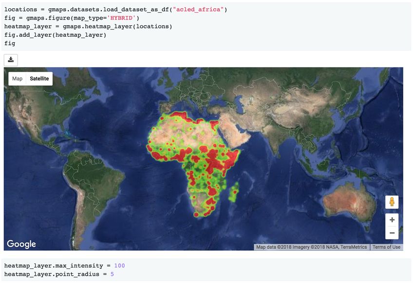
CHAPTER         1

                                                                                                   Installation

1.1 Installing jupyter-gmaps with conda

The easiest way to install gmaps is with conda:

$ conda install -c conda-forge gmaps

1.2 Installing jupyter-gmaps with pip

Make sure that you have enabled ipywidgets widgets extensions:

$ jupyter nbextension enable --py --sys-prefix widgetsnbextension

You can then install gmaps with:

$ pip install gmaps

Then tell Jupyter to load the extension with:

$ jupyter nbextension enable --py --sys-prefix gmaps

1.3 Installing jupyter-gmaps for JupyterLab

To use jupyter-gmaps with JupyterLab, you will need to install the jupyter widgets extension for JupyterLab:

$ jupyter labextension install @jupyter-widgets/jupyterlab-manager

You can then install jupyter-gmaps via pip (or conda):

                                                                                                               1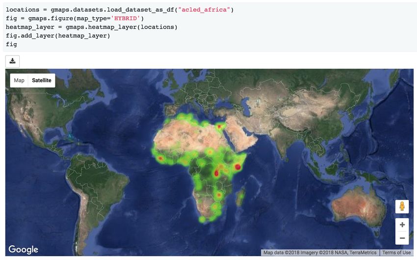
gmaps Documentation, Release 0.8.3-dev

$ pip install gmaps

Next time you open JupyterLab, you will be prompted to rebuild JupyterLab: this is necessary to include the jupyter-
gmaps frontend code into your JupyterLab installation. You can also trigger this directly on the command line with:

$ jupyter lab build

1.4 Development version

You must have NPM to install the development version. You can install NPM with your package manager.
We strongly recommend installing jupyter-gmaps in a virtual environment (either a conda environment or a virtualenv
environment).
Clone the git repository by running:

$ git clone https://github.com/pbugnion/gmaps.git

For the initial installation, run:

$ ./dev-install

This installs gmaps in editable mode and installs the Javascript components as symlinks.
If you then make changes to the code, you can make those changes available to a running notebook server by:
    • restarting the kernel if you have made changes to the Python source code
    • running npm run build:nbextension in the js/ directory and refreshing the browser page containing
      the notebook if you have made changes to the JavaScript source. You do not need to restart the kernel. If you are
      making many changes to the JavaScript directory, you can run npm run build:watch to rebuild on every
      change.
You should not need to restart the notebook server.

1.5 Source code

The jupyter-gmaps source is available on GitHub.

2                                                                                          Chapter 1. Installation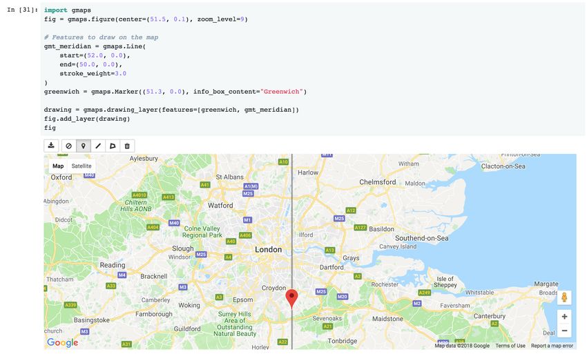
CHAPTER              2

                                                                                               Authentication

Most operations on Google Maps require that you tell Google who you are. To authenticate with Google Maps, follow
the instructions for creating an API key. You will probably want to create a new project, then click on the Credentials
section and create a Browser key. The API key is a string that starts with the letters AI.

You can pass this key to gmaps with the configure method:

gmaps.configure(api_key="AI...")

Maps and layers created after the call to gmaps.configure will have access to the API key.
You should avoid hard-coding the API key into your Jupyter notebooks. You can use environment variables. Add the
following line to your shell start-up file (probably ~/.profile or ~/.bashrc):

export GOOGLE_API_KEY=AI...

Make sure you don’t put spaces around the = sign. If you then open a new terminal window and type env at the
command prompt, you should see that your API key. Start a new Jupyter notebook server in a new terminal, and type:

import os
import gmaps
                                                                                                   (continues on next page)

                                                                                                                         3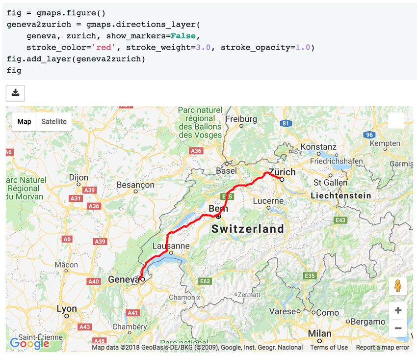
gmaps Documentation, Release 0.8.3-dev

                                                            (continued from previous page)

gmaps.configure(api_key=os.environ["GOOGLE_API_KEY"])

4                                                       Chapter 2. Authentication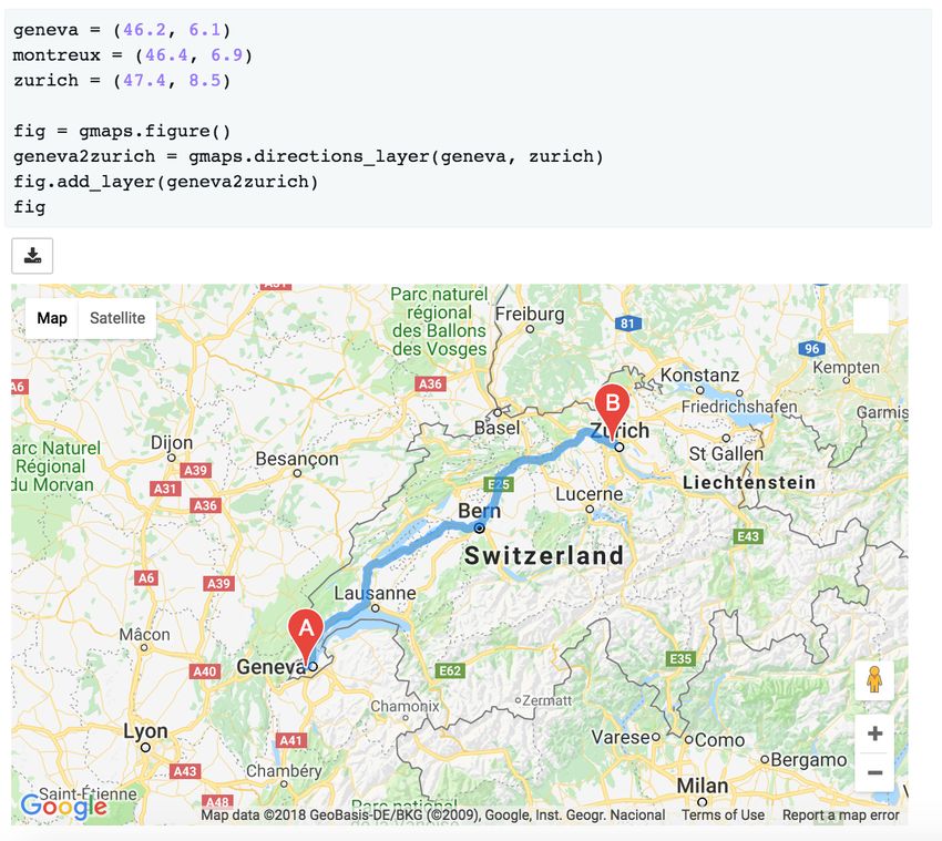
CHAPTER 3
Getting started
gmaps is a plugin for Jupyter for embedding Google Maps in your notebooks. It is designed as a data visualization
tool.
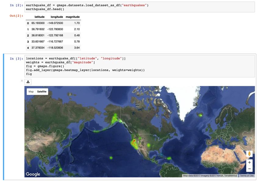
To demonstrate gmaps, let’s plot the earthquake dataset, included in the package:
import gmaps
import gmaps.datasets
gmaps.configure(api_key='AI...') # Fill in with your API key
earthquake_df = gmaps.datasets.load_dataset_as_df('earthquakes')
earthquake_df.head()
The earthquake data has three columns: a latitude and longitude indicating the earthquake’s epicentre and a weight
denoting the magnitude of the earthquake at that point. Let’s plot the earthquakes on a Google map:
locations = earthquake_df[['latitude', 'longitude']]
weights = earthquake_df['magnitude']
fig = gmaps.figure()
fig.add_layer(gmaps.heatmap_layer(locations, weights=weights))
fig
5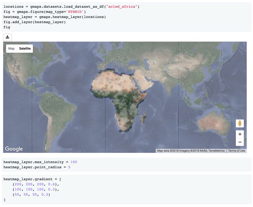
gmaps Documentation, Release 0.8.3-dev

This gives you a fully-fledged Google map. You can zoom in and out, switch to satellite view and even to street view
if you really want. The heatmap adjusts as you zoom in and out.

3.1 Basic concepts

gmaps is built around the idea of adding layers to a base map. After you’ve authenticated with Google maps, you start
by creating a figure, which contains a base map:

import gmaps
gmaps.configure(api_key='AI...')

fig = gmaps.figure()
fig

6                                                                                    Chapter 3. Getting started
gmaps Documentation, Release 0.8.3-dev

You then add layers on top of the base map. For instance, to add a heatmap layer:

import gmaps
gmaps.configure(api_key='AI...')

fig = gmaps.figure(map_type='SATELLITE')

# generate some (latitude, longitude) pairs
locations = [(51.5, 0.1), (51.7, 0.2), (51.4, -0.2), (51.49, 0.1)]

heatmap_layer = gmaps.heatmap_layer(locations)
fig.add_layer(heatmap_layer)
fig

3.1. Basic concepts                                                                                     7
gmaps Documentation, Release 0.8.3-dev

The locations array can either be a list of tuples, as in the example above, a numpy array of shape $N times 2$ or a
dataframe with two columns.
Most attributes on the base map and the layers can be set through named arguments in the constructor or as instance
attributes once the instance is created. These two constructions are thus equivalent:
heatmap_layer = gmaps.heatmap_layer(locations)
heatmap_layer.point_radius = 8

and:
heatmap_layer = gmaps.heatmap_layer(locations, point_radius=8)

The former construction is useful for modifying a map once it has been built. Any change in parameters will propagate
to maps in which those layers are included.

8                                                                                    Chapter 3. Getting started
gmaps Documentation, Release 0.8.3-dev

3.2 Base maps

Your first action with gmaps will usually be to build a base map:

import gmaps
gmaps.configure(api_key='AI...')

gmaps.figure()

This builds an empty map. You can also set the zoom level and map center explicitly:

new_york_coordinates = (40.75, -74.00)
gmaps.figure(center=new_york_coordinates, zoom_level=12)

If you do not set the map zoom and center, the viewport will automatically focus on the data as you add it to the map.
Google maps offers three different base map types. Choose the base map type by setting the map_type parameter:

gmaps.figure(map_type='HYBRID')

3.2. Base maps                                                                                                      9
gmaps Documentation, Release 0.8.3-dev

gmaps.figure(map_type='TERRAIN')

There are four map types available:
     • 'ROADMAP' is the default Google Maps style,

10                                                   Chapter 3. Getting started
gmaps Documentation, Release 0.8.3-dev
• 'SATELLITE' is a simple satellite view,
• 'HYBRID' is a satellite view with common features, such as roads and cities, overlaid,
• 'TERRAIN' is a map that emphasizes terrain features.
3.3 Customising map width, height and layout
The layout of a map figure is controlled by passing a layout argument. This is a dictionary of properties controlling
how the widget is displayed:
import gmaps
gmaps.configure(api_key='AI...')
figure_layout = {
'width': '400px',
'height': '400px',
'border': '1px solid black',
'padding': '1px'
}
gmaps.figure(layout=figure_layout)
The parameters that you are likely to want to tweak are:
• width: controls the figure width. This should be a CSS dimension. For instance, 400px will create a figure that
is 400 pixels wide, while 100% will create a figure that takes up the output cell’s entire width. The default width
is 100%.
• height: controls the figure height. This should be a CSS dimension. The default height is 420px.
• border: Place a border around the figure. This should be a valid CSS border.
• padding: Gap between the figure and the border. This should be a valid CSS padding. You can either have a
single dimension (e.g. 2px), or a quadruple indicating the padding width for each side (e.g. 1px 2px 1px
3.3. Customising map width, height and layout 11gmaps Documentation, Release 0.8.3-dev
2px). This is 0 by default.
• margin: Gap between the border and the figure container. This should be a valid CSS margin. This is 0 by
default.
To center a map in an output cell, use a fixed width and set the left and right margins to auto:
figure_layout = {'width': '500px', 'margin': '0 auto 0 auto'}
gmaps.figure(layout=figure_layout)
3.4 Heatmaps
Heatmaps are a good way of getting a sense of the density and clusters of geographical events. They are a powerful
tool for making sense of larger datasets. We will use a dataset recording all instances of political violence that occurred
in Africa between 1997 and 2015. The dataset comes from the Armed Conflict Location and Event Data Project. This
dataset contains about 110,000 rows.
import gmaps.datasets
locations = gmaps.datasets.load_dataset_as_df('acled_africa')
locations.head()
# => dataframe with 'longitude' and 'latitude' columns
We already know how to build a heatmap layer:
import gmaps
import gmaps.datasets
gmaps.configure(api_key='AI...')
locations = gmaps.datasets.load_dataset_as_df('acled_africa')
(continues on next page)
12 Chapter 3. Getting startedgmaps Documentation, Release 0.8.3-dev
(continued from previous page)
fig = gmaps.figure(map_type='HYBRID')
heatmap_layer = gmaps.heatmap_layer(locations)
fig.add_layer(heatmap_layer)
fig
3.4.1 Preventing dissipation on zoom
If you zoom in sufficiently, you will notice that individual points disappear. You can prevent this from happening
by controlling the max_intensity setting. This caps off the maximum peak intensity. It is useful if your data is
strongly peaked. This settings is None by default, which implies no capping. Typically, when setting the maximum
intensity, you also want to set the point_radius setting to a fairly low value. The only good way to find reasonable
values for these settings is to tweak them until you have a map that you are happy with.:
heatmap_layer.max_intensity = 100
heatmap_layer.point_radius = 5
To avoid re-drawing the whole map every time you tweak these settings, you may want to set them in another noteo-
book cell:
3.4. Heatmaps 13gmaps Documentation, Release 0.8.3-dev
Google maps also exposes a dissipating option, which is true by default. If this is true, the radius of influence
of each point is tied to the zoom level: as you zoom out, a given point covers more physical kilometres. If you set it
to false, the physical radius covered by each point stays fixed. Your points will therefore either be tiny at high zoom
levels or large at low zoom levels.
3.4.2 Setting the color gradient and opacity
You can set the color gradient of the map by passing in a list of colors. Google maps will interpolate linearly between
those colors. You can represent a color as a string denoting the color (the colors allowed by this):
heatmap_layer.gradient = [
'white',
'silver',
'gray'
]
If you need more flexibility, you can represent colours as an RGB triple or an RGBA quadruple:
heatmap_layer.gradient = [
(200, 200, 200, 0.6),
(100, 100, 100, 0.3),
(50, 50, 50, 0.3)
]
14 Chapter 3. Getting startedgmaps Documentation, Release 0.8.3-dev
You can also use the opacity option to set a single opacity across the entire colour gradient:
heatmap_layer.opacity = 0.0 # make the heatmap transparent
3.5 Weighted heatmaps
By default, heatmaps assume that every row is of equal importance. You can override this by passing weights through
the weights keyword argument. The weights array is an iterable (e.g. a Python list or a Numpy array) or a single
pandas series. Weights must all be positive (this is a limitation in Google maps itself).
import gmaps
import gmaps.datasets
gmaps.configure(api_key='AI...')
df = gmaps.datasets.load_dataset_as_df('earthquakes')
# dataframe with columns ('latitude', 'longitude', 'magnitude')
fig = gmaps.figure()
heatmap_layer = gmaps.heatmap_layer(
(continues on next page)
3.5. Weighted heatmaps 15gmaps Documentation, Release 0.8.3-dev
(continued from previous page)
df[['latitude', 'longitude']], weights=df['magnitude'],
max_intensity=30, point_radius=3.0
)
fig.add_layer(heatmap_layer)
fig
3.6 Markers and symbols
We can add a layer of markers to a Google map. Each marker represents an individual data point:
import gmaps
gmaps.configure(api_key='AI...')
marker_locations = [
(-34.0, -59.166672),
(-32.23333, -64.433327),
(40.166672, 44.133331),
(51.216671, 5.0833302),
(51.333328, 4.25)
]
(continues on next page)
16 Chapter 3. Getting startedgmaps Documentation, Release 0.8.3-dev
(continued from previous page)
fig = gmaps.figure()
markers = gmaps.marker_layer(marker_locations)
fig.add_layer(markers)
fig
We can also attach a pop-up box to each marker. Clicking on the marker will bring up the info box. The content of the
box can be either plain text or html:
import gmaps
gmaps.configure(api_key='AI...')
nuclear_power_plants = [
{'name': 'Atucha', 'location': (-34.0, -59.167), 'active_reactors': 1},
{'name': 'Embalse', 'location': (-32.2333, -64.4333), 'active_reactors': 1},
{'name': 'Armenia', 'location': (40.167, 44.133), 'active_reactors': 1},
{'name': 'Br', 'location': (51.217, 5.083), 'active_reactors': 1},
{'name': 'Doel', 'location': (51.333, 4.25), 'active_reactors': 4},
{'name': 'Tihange', 'location': (50.517, 5.283), 'active_reactors': 3}
]
plant_locations = [plant['location'] for plant in nuclear_power_plants]
info_box_template = """
Name{name}
Number reactors{active_reactors}
"""
plant_info = [info_box_template.format(**plant) for plant in nuclear_power_plants]
marker_layer = gmaps.marker_layer(plant_locations, info_box_content=plant_info)
fig = gmaps.figure()
fig.add_layer(marker_layer)
(continues on next page)
3.6. Markers and symbols 17gmaps Documentation, Release 0.8.3-dev
(continued from previous page)
fig
Markers are currently limited to the Google maps style drop icon. If you need to draw more complex shape on maps,
use the symbol_layer function. Symbols represent each latitude, longitude pair with a circle whose colour and
size you can customize. Let’s, for instance, plot the location of every Starbuck’s coffee shop in the UK:
import gmaps
import gmaps.datasets
gmaps.configure(api_key='AI...')
df = gmaps.datasets.load_dataset_as_df('starbucks_kfc_uk')
starbucks_df = df[df['chain_name'] == 'starbucks']
starbucks_df = starbucks_df[['latitude', 'longitude']]
starbucks_layer = gmaps.symbol_layer(
starbucks_df, fill_color='green', stroke_color='green', scale=2
)
fig = gmaps.figure()
fig.add_layer(starbucks_layer)
fig
18 Chapter 3. Getting startedgmaps Documentation, Release 0.8.3-dev
You can have several layers of markers. For instance, we can compare the locations of Starbucks coffee shops and
KFC outlets in the UK by plotting both on the same map:
import gmaps
import gmaps.datasets
gmaps.configure(api_key='AI...')
df = gmaps.datasets.load_dataset_as_df('starbucks_kfc_uk')
starbucks_df = df[df['chain_name'] == 'starbucks']
starbucks_df = starbucks_df[['latitude', 'longitude']]
kfc_df = df[df['chain_name'] == 'kfc']
kfc_df = kfc_df[['latitude', 'longitude']]
starbucks_layer = gmaps.symbol_layer(
starbucks_df, fill_color='rgba(0, 150, 0, 0.4)',
stroke_color='rgba(0, 150, 0, 0.4)', scale=2
)
kfc_layer = gmaps.symbol_layer(
kfc_df, fill_color='rgba(200, 0, 0, 0.4)',
stroke_color='rgba(200, 0, 0, 0.4)', scale=2
)
fig = gmaps.figure()
fig.add_layer(starbucks_layer)
fig.add_layer(kfc_layer)
fig
3.6. Markers and symbols 19gmaps Documentation, Release 0.8.3-dev
3.6.1 Dataset size limitations
Google maps may become very slow if you try to represent more than a few thousand symbols or markers. If you have
a larger dataset, you should either consider subsampling or use heatmaps.
3.7 GeoJSON layer
We can add GeoJSON to a map. This is very useful when we want to draw chloropleth maps.
You can either load data from your own GeoJSON file, or you can load one of the GeoJSON geometries bundled with
gmaps. Let’s start with the latter. We will create a map of the GINI coefficient (a measure of inequality) for every
country in the world.
Let’s start by just plotting the raw GeoJSON:
import gmaps
import gmaps.geojson_geometries
gmaps.configure(api_key='AIza...')
countries_geojson = gmaps.geojson_geometries.load_geometry('countries')
(continues on next page)
20 Chapter 3. Getting startedgmaps Documentation, Release 0.8.3-dev
(continued from previous page)
fig = gmaps.figure()
gini_layer = gmaps.geojson_layer(countries_geojson)
fig.add_layer(gini_layer)
fig
This just plots the country boundaries on top of a Google map.
Next, we want to colour each country by a colour derived from its GINI index. We first need to map from each item
in the GeoJSON document to a GINI value. GeoJSON documents are organised as a collection of features, each of
which has the keys geometry and properties. For instance, for our countries:
>>> print(len(geojson['features']))
217 # corresponds to 217 distinct countries and territories
>>> print(geojson['features'][0])
{
'type': 'Feature'
'geometry': {'coordinates': [ ... ], 'type': 'Polygon'},
'properties': {'ISO_A3': u'AFG', 'name': u'Afghanistan'}
}
As we can see, properties encodes meta-information about the feature, like the country name. We will use this name
to look up a GINI value for that country and translate that into a colour. We can download a list of GINI coefficients
for (nearly) every country using the gmaps.datasets module (you could load your own data here):
import gmaps.datasets
rows = gmaps.datasets.load_dataset('gini') # 'rows' is a list of tuples
country2gini = dict(rows) # dictionary mapping 'country' -> gini coefficient
(continues on next page)
3.7. GeoJSON layer 21gmaps Documentation, Release 0.8.3-dev
(continued from previous page)
print(country2gini['United Kingdom'])
# 32.4
We can now use the country2gini dictionary to map each country to a color. We will use a Matplotlib colormap
to map from our GINI floats to a color that makes sense on a linear scale. We will use the Viridis colorscale:
from matplotlib.cm import viridis
from matplotlib.colors import to_hex
# We will need to scale the GINI values to lie between 0 and 1
min_gini = min(country2gini.values())
max_gini = max(country2gini.values())
gini_range = max_gini - min_gini
def calculate_color(gini):
"""
Convert the GINI coefficient to a color
"""
# make gini a number between 0 and 1
normalized_gini = (gini - min_gini) / gini_range
# invert gini so that high inequality gives dark color
inverse_gini = 1.0 - normalized_gini
# transform the gini coefficient to a matplotlib color
mpl_color = viridis(inverse_gini)
# transform from a matplotlib color to a valid CSS color
gmaps_color = to_hex(mpl_color, keep_alpha=False)
return gmaps_color
We now need to build an array of colors, one for each country, that we can pass to the GeoJSON layer. The easiest
way to do this is to iterate over the array of features in the GeoJSON:
colors = []
for feature in countries_geojson['features']:
country_name = feature['properties']['name']
try:
gini = country2gini[country_name]
color = calculate_color(gini)
except KeyError:
# no GINI for that country: return default color
color = (0, 0, 0, 0.3)
colors.append(color)
We can now pass our array of colors to the GeoJSON layer:
fig = gmaps.figure()
gini_layer = gmaps.geojson_layer(
countries_geojson,
fill_color=colors,
stroke_color=colors,
fill_opacity=0.8)
fig.add_layer(gini_layer)
fig
22 Chapter 3. Getting startedgmaps Documentation, Release 0.8.3-dev
3.7.1 GeoJSON geometries bundled with Gmaps
Finding appropriate GeoJSON geometries can be painful. To mitigate this somewhat, gmaps comes with its own set
of curated GeoJSON geometries:
>>> import gmaps.geojson_geometries
>>> gmaps.geojson_geometries.list_geometries()
['brazil-states',
'england-counties',
'us-states',
'countries',
'india-states',
'us-counties',
'countries-high-resolution']
>>> gmaps.geojson_geometries.geometry_metadata('brazil-states')
{'description': 'US county boundaries',
'source': 'http://eric.clst.org/Stuff/USGeoJSON'}
Use the load_geometry function to get the GeoJSON object:
import gmaps
import gmaps.geojson_geometries
gmaps.configure(api_key='AIza...')
countries_geojson = gmaps.geojson_geometries.load_geometry('brazil-states')
(continues on next page)
3.7. GeoJSON layer 23gmaps Documentation, Release 0.8.3-dev
(continued from previous page)
fig = gmaps.figure()
geojson_layer = gmaps.geojson_layer(countries_geojson)
fig.add_layer(geojson_layer)
fig
New geometries would greatly enhance the usability of jupyter-gmaps. Refer to this issue on GitHub for information
on how to contribute a geometry.
3.7.2 Loading your own GeoJSON
So far, we have only considered visualizing GeoJSON geometries that come with jupyter-gmaps. Most of the time,
though, you will want to load your own geometry. Use the standard library json module for this:
import json
import gmaps
gmaps.configure(api_key='AIza...')
with open('my_geojson_geometry.json') as f:
geometry = json.load(f)
fig = gmaps.figure()
geojson_layer = gmaps.geojson_layer(geometry)
fig.add_layer(geojson_layer)
fig
3.8 Drawing markers, lines and polygons
The drawing layer lets you draw complex shapes on the map. You can add markers, lines and polygons directly to
maps. Let’s, for instance, draw the Greenwich meridian and add a marker on Greenwich itself:
import gmaps
gmaps.configure(api_key='AIza...')
fig = gmaps.figure(center=(51.5, 0.1), zoom_level=9)
# Features to draw on the map
gmt_meridian = gmaps.Line(
start=(52.0, 0.0),
end=(50.0, 0.0),
stroke_weight=3.0
)
greenwich = gmaps.Marker((51.3, 0.0), info_box_content='Greenwich')
drawing = gmaps.drawing_layer(features=[greenwich, gmt_meridian])
fig.add_layer(drawing)
fig
24 Chapter 3. Getting startedgmaps Documentation, Release 0.8.3-dev
Adding the drawing layer to a map displays drawing controls that lets users add arbitrary shapes to the map. This is
useful if you want to react to user events (for instance, if you want to run some Python code every time the user adds
a marker). This is discussed in the Reacting to user actions on the map section.
To hide the drawing controls, pass show_controls=False as argument to the drawing layer:
drawing = gmaps.drawing_layer(
features=[greenwich, gmt_meridian],
show_controls=False
)
Besides lines and markers, you can also draw polygons on the map. This is useful for drawing complex shapes. For
instance, we can draw the London congestion charge zone. jupyter-gmaps has a built-in dataset with the coordinates
of this zone:
import gmaps
import gmaps.datasets
london_congestion_zone_path = gmaps.datasets.load_dataset('london_congestion_zone')
london_congestion_zone_path[:2]
# [(51.530318, -0.123026), (51.530078, -0.123614)]
We can draw this on the map with a gmaps.Polygon:
fig = gmaps.figure(center=(51.5, -0.1), zoom_level=12)
london_congestion_zone_polygon = gmaps.Polygon(
london_congestion_zone_path,
stroke_color='blue',
fill_color='blue'
)
drawing = gmaps.drawing_layer(
(continues on next page)
3.8. Drawing markers, lines and polygons 25gmaps Documentation, Release 0.8.3-dev
(continued from previous page)
features=[london_congestion_zone_polygon],
show_controls=False
)
fig.add_layer(drawing)
fig
We can pass an arbitrary list of (latitude, longitude) pairs to gmaps.Polygon to specify complex shapes. For details on
how to style polygons, see the gmaps.Polygon API documentation.
See the API documentation for gmaps.drawing_layer() for an exhaustive list of options for the drawing layer.
3.9 Directions layer
gmaps supports drawing routes based on the Google maps directions service. At the moment, this only supports
directions between points denoted by latitude and longitude:
import gmaps
import gmaps.datasets
gmaps.configure(api_key='AIza...')
# Latitude-longitude pairs
geneva = (46.2, 6.1)
montreux = (46.4, 6.9)
zurich = (47.4, 8.5)
fig = gmaps.figure()
geneva2zurich = gmaps.directions_layer(geneva, zurich)
(continues on next page)
26 Chapter 3. Getting startedgmaps Documentation, Release 0.8.3-dev
(continued from previous page)
fig.add_layer(geneva2zurich)
fig
You can also pass waypoints and customise the directions request. You can pass up to 23 waypoints. Waypoints are
not supported when the travel mode is 'TRANSIT' (this is a limitation of the Google Maps directions service):
fig = gmaps.figure()
geneva2zurich_via_montreux = gmaps.directions_layer(
geneva, zurich, waypoints=[montreux],
travel_mode='BICYCLING')
fig.add_layer(geneva2zurich_via_montreux)
fig
3.9. Directions layer 27gmaps Documentation, Release 0.8.3-dev
You can customise how directions are rendered on the map:
fig = gmaps.figure()
geneva2zurich = gmaps.directions_layer(
geneva, zurich, show_markers=False,
stroke_color='red', stroke_weight=3.0, stroke_opacity=1.0)
fig.add_layer(geneva2zurich)
fig
28 Chapter 3. Getting startedgmaps Documentation, Release 0.8.3-dev The full list of options is given as part of the documentation for the gmaps.directions_layer(). Updating options on the layer object will update the map. This lets you use the directions layer as part of a larger widget application. See the app tutorial for details. 3.10 Bicycling, transit and traffic layers You can add bicycling, transit and traffic information to a base map. For instance, use gmaps. bicycling_layer() to draw cycle lanes. This will also change the style of the base layer to de-emphasize streets which are not cycle-friendly. import gmaps gmaps.configure(api_key='AI...') # Map centered on London fig = gmaps.figure(center=(51.5, -0.2), zoom_level=11) fig.add_layer(gmaps.bicycling_layer()) fig 3.10. Bicycling, transit and traffic layers 29
gmaps Documentation, Release 0.8.3-dev

Similarly, the transit layer, available as gmaps.transit_layer(), adds information about public transport, where
available.

30                                                                               Chapter 3. Getting started
gmaps Documentation, Release 0.8.3-dev

The traffic layer, available as gmaps.traffic_layer(), adds information about the current state of traffic.

3.10. Bicycling, transit and traffic layers                                                                   31
gmaps Documentation, Release 0.8.3-dev

Unlike the other layers, these layers do not take any user data. Thus, jupyter-gmaps will not use them to center the
map. This means that, if you use these layers by themselves, you will often want to center the figure explicitly, using
the center and zoom_level attributes.

32                                                                                    Chapter 3. Getting started
CHAPTER              4

                                                     Building applications with jupyter-gmaps

You can use jupyter-gmaps as a component in a Jupyter widgets application. Jupyter widgets let you embed rich user interfaces i

          • you can use maps as a way to get user input. The drawing layer lets users draw markers, lines or polygons
            on the map. We can specify arbitrary Python code that runs whenever a shape is added to the map. As an
            example, we will build an application where, whenever the user places a marker, we retrieve the address
            of the marker and write it in a text widget.
          • you can use maps as a way to display the result of an external computation. For instance, if you have
            timestamped geographical data (for instance, you have the date and coordinates of a series of events), you
            can combine a heatmap with a slider to see how events unfold over time.

4.1 Reacting to user actions on the map

The drawing layer lets us specify Python code to be executed whenever the user adds a feature (like a marker, a line
or a polygon) to the map. To demonstrate this, we will build a small application for reverse geocoding: when the user
places a marker on the map, we will find the address closest to that marker and write it in a text widget. We will use
geopy, a wrapper around several geocoding APIs, to calculate the address from the marker’s coordinates.
This is the entire code listing:

import ipywidgets as widgets
import geopy
import gmaps

API_KEY = 'AIz...'

gmaps.configure(api_key=API_KEY)

class ReverseGeocoder(object):
    """
    Jupyter widget for finding addresses.
                                                                                                  (continues on next page)

                                                                                                                      33
gmaps Documentation, Release 0.8.3-dev
(continued from previous page)
The user places markers on a map. For each marker,
we use `geopy` to find the nearest address to that
marker, and write that address in a text box.
"""
def __init__(self):
self._figure = gmaps.figure()
self._drawing = gmaps.drawing_layer()
self._drawing.on_new_feature(self._new_feature_callback)
self._figure.add_layer(self._drawing)
self._address_box = widgets.Text(
description='Address: ',
disabled=True,
layout={'width': '95%', 'margin': '10px 0 0 0'}
)
self._geocoder = geopy.geocoders.GoogleV3(api_key=API_KEY)
self._container = widgets.VBox([self._figure, self._address_box])
def _get_location_details(self, location):
return self._geocoder.reverse(location, exactly_one=True)
def _clear_address_box(self):
self._address_box.value = ''
def _show_address(self, location):
location_details = self._get_location_details(location)
if location_details is None:
self._address_box.value = 'No address found'
else:
self._address_box.value = location_details.address
def _new_feature_callback(self, feature):
try:
location = feature.location
except AttributeError:
return # Not a marker
# Clear address box to signify to the user that something is happening
self._clear_address_box()
# Remove all markers other than the one that has just been added.
self._drawing.features = [feature]
# Compute the address and display it
self._show_address(location)
def render(self):
return self._container
ReverseGeocoder().render()
34 Chapter 4. Building applications with jupyter-gmapsgmaps Documentation, Release 0.8.3-dev
There are several things to note:
• We wrap the application in a ReverseGeocoder class. Wrapping your application in a class (rather than
using the notebook’s global namespace) helps with encapsulation and lets you instantiate this widget multiple
times. Since the flow through widget applications is often more complex than linear data analysis workflows,
encapsulation will improve your ability to reason about the code.
• As part of the class constructor, we use gmaps.figure() to create a figure. We then use gmaps.
drawing_layer() to create a drawing layer, which we add to the figure. We also create a widgets.Text
widget. This is a text box in which we will write the address. We then wrap our figure and the text box in a
single widgets.VBox, a widget container that stacks widgets vertically.
• We register a callback on the drawing layer using .on_new_feature. The function that we pass in to .
on_new_feature will get called whenever the user adds a feature to the map. This is the hook that lets us
build complex applications on top of the drawing layer: we can run arbitrary Python code when the user adds a
marker to the map.
• In the .on_new_feature callback, we first check whether the feature that has been added is a marker (the
user could, in principle, have added another feature type, like a line, to the map).
• Assuming the feature is a valid marker, we first clear the text widget containing the address. This gives feedback
to the user that something is happening.
• We then re-write the .features array of the drawing layer, keeping just the marker that the user has just
added. This clears previous markers, avoiding clutter on the map.
• We then use geopy to find the adddress. Assuming the address is valid, display it in the text widget.
4.1. Reacting to user actions on the map 35gmaps Documentation, Release 0.8.3-dev
4.2 Updating a heatmap in response to other widgets
Many layers support updating the data without re-rendering the entire map. This is useful for exploring multi-
dimensional datasets, especially in conjunction with other widgets.
As an example, we will use the acled_africa_by_year dataset, a dataset indexing violence against civilians in
Africa. The original dataset is from the ACLED project. The dataset has four columns:
import gmaps.datasets
df = gmaps.datasets.load_dataset_as_df('acled_africa_by_year')
df.head()
We will build an application that lets the user explore different years via a slider. When the user changes the slider, we
display the total number of fatalities for that year, and update a heatmap showing the distribution of conflicts.
This is the entire code listing:
from IPython.display import display
import ipywidgets as widgets
import gmaps
gmaps.configure(api_key='AIza...')
class AcledExplorer(object):
"""
Jupyter widget for exploring the ACLED dataset.
The user uses the slider to choose a year. This renders
a heatmap of civilian victims in that year.
"""
def __init__(self, df):
self._df = df
self._heatmap = None
self._slider = None
initial_year = min(self._df['year'])
title_widget = widgets.HTML(
'Civilian casualties in Africa, by year'
'Data from ACLED project
˓→ '
)
map_figure = self._render_map(initial_year)
controls = self._render_controls(initial_year)
(continues on next page)
36 Chapter 4. Building applications with jupyter-gmapsgmaps Documentation, Release 0.8.3-dev
(continued from previous page)
self._container = widgets.VBox([title_widget, controls, map_figure])
def render(self):
display(self._container)
def _on_year_change(self, change):
year = self._slider.value
self._heatmap.locations = self._locations_for_year(year)
self._total_box.value = self._total_casualties_text_for_year(year)
return self._container
def _render_map(self, initial_year):
fig = gmaps.figure(map_type='HYBRID')
self._heatmap = gmaps.heatmap_layer(
self._locations_for_year(initial_year),
max_intensity=100,
point_radius=8
)
fig.add_layer(self._heatmap)
return fig
def _render_controls(self, initial_year):
self._slider = widgets.IntSlider(
value=initial_year,
min=min(self._df['year']),
max=max(self._df['year']),
description='Year',
continuous_update=False
)
self._total_box = widgets.Label(
value=self._total_casualties_text_for_year(initial_year)
)
self._slider.observe(self._on_year_change, names='value')
controls = widgets.HBox(
[self._slider, self._total_box],
layout={'justify_content': 'space-between'}
)
return controls
def _locations_for_year(self, year):
return self._df[self._df['year'] == year][['latitude', 'longitude']]
def _total_casualties_for_year(self, year):
return int(self._df[self._df['year'] == year]['year'].count())
def _total_casualties_text_for_year(self, year):
return '{} civilian casualties'.format(self._total_casualties_for_year(year))
AcledExplorer(df).render()
4.2. Updating a heatmap in response to other widgets 37gmaps Documentation, Release 0.8.3-dev
There are several things to note on this:
• We wrap the application in a class to help keep the mutable state encapsulated.
• As part of the class constructor, we use gmaps.figure() to create a figure. We add use gmaps.
heatmap_layer() to create a heatmap, which we add to the figure. The Heatmap object returned has
a locations attribute. Setting this to a new value will automatically update the heatmap.
• We create a slider with widgets.IntSlider. In general, jupyter-gmaps objects are designed to interact
with widgets from ipywidgets. For a full list of available widgets, see the ipywidgets documentation.
• We want to react to changes in the slider: every time the slider moves, we recompute the total number of
fatalities and update the data in the heatmap. To react to changes in a widget, we use the .observe method on
the widget. This lets us specify a callback that gets called whenever a given attribute of the widget changes. We
pass the names="value" argument to slider.observe to only react to changes in the slider’s value
attribute. Note that the callback (self.render in our case) needs to take a single argument. It gets passed a
dictionary describing the change.
• To build the layout for our application, we use combinations of HBox and VBox widgets.
4.3 Updating symbols in response to other widgets
The marker and symbol layers can also be udpated dynamically (as can most other markers).
As an example, we will use the starbucks_kfc_uk dataset, a dataset indexing the location of every Starbucks and
KFC in the UK. The original dataset is from the UK food standards agency.
We will build a application with two checkboxes, one for Starbucks outlets and one for KFC outlets. We react to users
clicking on the outlets by changing the symbols displayed on the map.
This is the entire code listing:
38 Chapter 4. Building applications with jupyter-gmapsgmaps Documentation, Release 0.8.3-dev
from IPython.display import display
import ipywidgets as widgets
import gmaps
import gmaps.datasets
gmaps.configure(api_key="AIza...")
class OutletExplorer(object):
def __init__(self, df):
"""
Jupyter widget for exploring KFC and Starbucks outlets
Using checkboxes, the user chooses whether to include
Starbucks, KFC outlets, both or neither.
"""
self._df = df
self._symbol_layer = None
self._starbucks_symbols = self._create_symbols_for_chain(
'starbucks', 'rgba(0, 150, 0, 0.4)')
self._kfc_symbols = self._create_symbols_for_chain(
'kfc', 'rgba(150, 0, 0, 0.4)')
title_widget = widgets.HTML(
'Explore KFC and Starbucks locations'
'Data from UK Food Standards Agency
˓→'
)
controls = self._render_controls(True, True)
map_figure = self._render_map(True, True)
self._container = widgets.VBox(
[title_widget, controls, map_figure])
def render(self):
""" Render the widget """
display(self._container)
def _render_map(self, initial_include_starbucks, initial_include_kfc):
""" Render the initial map """
fig = gmaps.figure(layout={'height': '500px'})
symbols = self._generate_symbols(True, True)
self._symbol_layer = gmaps.Markers(markers=symbols)
fig.add_layer(self._symbol_layer)
return fig
def _render_controls(
self,
initial_include_starbucks,
initial_include_kfc
):
""" Render the checkboxes """
self._starbucks_checkbox = widgets.Checkbox(
value=initial_include_starbucks,
description='Starbucks'
)
(continues on next page)
4.3. Updating symbols in response to other widgets 39gmaps Documentation, Release 0.8.3-dev
(continued from previous page)
self._kfc_checkbox = widgets.Checkbox(
value=initial_include_kfc,
description='KFC'
)
self._starbucks_checkbox.observe(
self._on_controls_change, names='value')
self._kfc_checkbox.observe(
self._on_controls_change, names='value')
controls = widgets.VBox(
[self._starbucks_checkbox, self._kfc_checkbox])
return controls
def _on_controls_change(self, obj):
"""
Called when the checkboxes change
This method builds the list of symbols to include on the map,
based on the current checkbox values. It then updates the
symbol layer with the new symbol list.
"""
include_starbucks = self._starbucks_checkbox.value
include_kfc = self._kfc_checkbox.value
symbols = self._generate_symbols(
include_starbucks, include_kfc)
# Update the layer with the new symbols:
self._symbol_layer.markers = symbols
def _generate_symbols(self, include_starbucks, include_kfc):
""" Generate the list of symbols to includs """
symbols = []
if include_starbucks:
symbols.extend(self._starbucks_symbols)
if include_kfc:
symbols.extend(self._kfc_symbols)
return symbols
def _create_symbols_for_chain(self, chain, color):
chain_df = self._df[self._df['chain_name'] == chain]
symbols = [
gmaps.Symbol(
location=(latitude, longitude),
stroke_color=color,
fill_color=color,
scale=2
)
for latitude, longitude in
zip(chain_df["latitude"], chain_df["longitude"])
]
return symbols
df = gmaps.datasets.load_dataset_as_df("starbucks_kfc_uk")
OutletExplorer(df).render()
40 Chapter 4. Building applications with jupyter-gmapsgmaps Documentation, Release 0.8.3-dev We used the gmaps.Markers class to represent the symbol layer, rather than the gmaps.symbol_layer() factory function. The Markers class is easier to manipulate, since it just takes a list of symbols. The disadvantage is that we had to construct the symbols independently. 4.3. Updating symbols in response to other widgets 41
gmaps Documentation, Release 0.8.3-dev

42                                       Chapter 4. Building applications with jupyter-gmaps
CHAPTER     5

                                                                                             Exporting maps

5.1 Exporting to PNG

You can save maps to PNG by clicking the Download button in the toolbar. This will download a static copy of the
map.
This feature suffers from some know issues:
    • there is no way to set the quality of the rendering at present,
    • you cannot export maps that contain a Directions layer (see the issue on Github for details).

5.2 Exporting to HTML

You can export maps to HTML using the infrastructure provided by ipywidgets. For instance, let’s export a simple
map to HTML:

from ipywidgets.embed import embed_minimal_html
import gmaps

gmaps.configure(api_key="AI...")

fig = gmaps.figure()
embed_minimal_html('export.html', views=[fig])

This generates a file, export.html, with two (or more)  tags that contain the widget state. The scripts
with tag  indicate where the wid-
gets will be placed in the DOM. You can move these around and nest them in other DOM elements to change where
the exported maps appear in the DOM.
Open export.html with a webserver, e.g. by running, if you use Python 3:

python -m http.server 8080

                                                                                                             43
gmaps Documentation, Release 0.8.3-dev Or, if you use Python 2: python -m SimpleHTTPServer 8080 Navigate to http://0.0.0.0:8080/export.html and you should see the export! The module ipywidgets.embed contains other functions for exporting that will give you greater control over what is exported. See the documentation and the source code for more details. 44 Chapter 5. Exporting maps
CHAPTER             6

                                                                                        API documentation

6.1 Figures and layers

gmaps.figure(display_toolbar=True, display_errors=True, zoom_level=None, tilt=45, center=None, lay-
                out=None, map_type=’ROADMAP’, mouse_handling=’COOPERATIVE’)
    Create a gmaps figure
     This returns a Figure object to which you can add data layers.
          Parameters
                 • display_toolbar (boolean, optional) – Boolean denoting whether to show the
                   toolbar. Defaults to True.
                 • display_errors (boolean, optional) – Boolean denoting whether to show er-
                   rors that arise in the client. Defaults to True.
                 • zoom_level (int, optional) – Integer between 0 and 21 indicating the initial zoom
                   level. High values are more zoomed in. By default, the zoom level is chosen to fit the data
                   passed to the map. If specified, you must also specify the map center.
                 • tilt (int, optional) – Tilt can be either 0 or 45 indicating the tilt angle in degrees.
                   45-degree imagery is only available for satellite and hybrid map types, and is not available at
                   every location at every zoom level. For locations where 45-degree imagery is not available,
                   Google Maps will automatically fall back to 0 tilt.
                 • center (tuple, optional) – Latitude-longitude pair determining the map center. By
                   default, the map center is chosen to fit the data passed to the map. If specified, you must
                   also specify the zoom level.
                 • map_type (str, optional) – String representing the type of map to show. One of
                   ‘ROADMAP’ (the classic Google Maps style) ‘SATELLITE’ (just satellite tiles with no
                   overlay), ‘HYBRID’ (satellite base tiles but with features such as roads and cities overlaid)
                   and ‘TERRAIN’ (map showing terrain features). Defaults to ‘ROADMAP’.
                 • mouse_handling (str, optional) – String representing how the map captures the
                   page’s mouse event. One of ‘COOPERATIVE’ (scroll events scroll the page without zoom-

                                                                                                                     45
gmaps Documentation, Release 0.8.3-dev
ing the map, double clicks or CTRL/CMD+scroll zoom the map), ‘GREEDY’ (the map
captures all scroll events), ‘NONE’ (the map cannot be zoomed or panned by user ges-
tures) or ‘AUTO’ (cooperative if the notebook is displayed in an iframe, greedy otherwise).
Defaults to ‘COOPERATIVE’.
• layout (dict, optional) – Control the layout of the figure, e.g. its width, height,
border etc. For instance, passing layout={'width': '400px', 'height':
'300px'} will build a figure of fixed width and height. For more in formation on available
properties, see the ipywidgets documentation on widget layout.
Returns A gmaps.Figure widget.
Examples
>>> import gmaps
>>> gmaps.configure(api_key="AI...")
>>> fig = gmaps.figure()
>>> locations = [(46.1, 5.2), (46.2, 5.3), (46.3, 5.4)]
>>> fig.add_layer(gmaps.heatmap_layer(locations))
You can also explicitly specify the intiial map center and zoom:
>>> fig = gmaps.figure(center=(46.0, -5.0), zoom_level=8)
To customise the layout:
>>> fig = gmaps.figure(layout={
'width': '400px',
'height': '600px',
'padding': '3px',
'border': '1px solid black'
})
To have a satellite map:
>>> fig = gmaps.figure(map_type='HYBRID')
gmaps.heatmap_layer(locations, weights=None, max_intensity=None, dissipating=True,
point_radius=None, opacity=0.6, gradient=None)
Create a heatmap layer.
This returns a gmaps.Heatmap or a gmaps.WeightedHeatmap object that can be added to a gmaps.
Figure to draw a heatmap. A heatmap shows the density of points in or near a particular area.
To set the parameters, pass them to the constructor or set them on the Heatmap object after construction:
>>> heatmap = gmaps.heatmap_layer(locations, max_intensity=10)
or:
>>> heatmap = gmaps.heatmap_layer(locations)
>>> heatmap.max_intensity = 10
Examples
>>> fig = gmaps.figure()
>>> locations = [(46.1, 5.2), (46.2, 5.3), (46.3, 5.4)]
>>> heatmap = gmaps.heatmap_layer(locations)
(continues on next page)
46 Chapter 6. API documentationgmaps Documentation, Release 0.8.3-dev
(continued from previous page)
>>> heatmap.max_intensity = 2
>>> heatmap.point_radius = 3
>>> heatmap.gradient = ['white', 'gray']
>>> fig.add_layer(heatmap)
Parameters
• locations (iterable of latitude, longitude pairs) – Iterable of (lati-
tude, longitude) pairs denoting a single point. Latitudes are expressed as a float between -90
(corresponding to 90 degrees south) and +90 (corresponding to 90 degrees north). Longi-
tudes are expressed as a float between -180 (corresponding to 180 degrees west) and +180
(corresponding to 180 degrees east). This can be passed in as either a list of tuples, a two-
dimensional numpy array or a pandas dataframe with two columns, in which case the first
one is taken to be the latitude and the second one is taken to be the longitude.
• weights (iterable of floats, optional) – Iterable of weights of the same
length as locations. All the weights must be positive.
• max_intensity (float, optional) – Strictly positive floating point number indi-
cating the numeric value that corresponds to the hottest colour in the heatmap gradient. Any
density of points greater than that value will just get mapped to the hottest colour. Setting
this value can be useful when your data is sharply peaked. It is also useful if you find that
your heatmap disappears as you zoom in.
• point_radius (int, optional) – Number of pixels for each point passed in the
data. This determines the “radius of influence” of each data point.
• dissipating (bool, optional) – Whether the radius of influence of each point
changes as you zoom in or out. If dissipating is True, the radius of influence of each point
increases as you zoom out and decreases as you zoom in. If False, the radius of influence
remains the same. Defaults to True.
• opacity (float, optional) – The opacity of the heatmap layer. Defaults to 0.6.
• gradient (list of colors, optional) – The color gradient for the heatmap.
This must be specified as a list of colors. Google Maps then interpolates linearly between
those colors. Colors can be specified as a simple string, e.g. ‘blue’, as an RGB tuple, e.g.
(100, 0, 0), or as an RGBA tuple, e.g. (100, 0, 0, 0.5).
Returns A gmaps.Heatmap or a gmaps.WeightedHeatmap widget.
gmaps.symbol_layer(locations, hover_text=”, fill_color=None, fill_opacity=1.0, stroke_color=None,
stroke_opacity=1.0, scale=3, info_box_content=None, display_info_box=None)
Symbol layer
Add this layer to a gmaps.Figure instance to draw symbols on the map. A symbol will be drawn on the map
for each point in the locations argument.
Examples
>>> fig = gmaps.figure()
>>> locations = [
(-34.0, -59.166672),
(-32.23333, -64.433327),
(40.166672, 44.133331),
(51.216671, 5.0833302),
(51.333328, 4.25)
]
(continues on next page)
6.1. Figures and layers 47You can also read