Ground Truth for the Future - Low Distortion Projections and the State Plane Coordinate System of 2022 - Arizona Professional Land ...
←
→
Page content transcription
If your browser does not render page correctly, please read the page content below

Arizona Professional Land Surveyors Association
                                  Flagstaff, Arizona | August 17, 2019

Ground Truth for the Future
Low Distortion Projections and the
State Plane Coordinate
System of 2022
Michael L. Dennis, PhD, PE, RLS
August 2019

Design and metadata example:            NOAA’s National Geodetic Survey
OCRS Bend-Redmond-Prineville              https://geodesy.noaa.gov
Ground Truth for the Future

Table of Contents
Workshop description and speaker biography ................................................................................ 2
Map projection types and conformality .......................................................................................... 3
Map projection distortion ................................................................................................................ 6
Methods for creating low-distortion projected coordinate systems .............................................. 10
Six steps illustrating Low Distortion Projection (LDP) design .................................................... 12
Design example for a Low Distortion Projection (LDP) .............................................................. 19
Projection grid scale factor and convergence angle computation ................................................. 31
Methods for computing horizontal “ground” distance.................................................................. 33
Surveying & mapping spatial data requirements & recommendations ........................................ 34
Example of surveying and mapping documentation (metadata) .................................................. 35
Selected References ...................................................................................................................... 36

List of Figures
Figure 1. Map projection developable surfaces and their projection axes. ................................... 4
Figure 2. Secant, tangent, and non-intersecting projection developable surfaces. ....................... 6
Figure 3. Linear distortion of secant map projection with respect to ellipsoid and topography ... 8
Figure 4. Comparison of (a) SPCS, (b) “modified” SPCS, and (c) LDP .................................... 11
Figure 5. LDP design area, showing topographic ellipsoid heights of towns ............................. 19
Figure 6. Linear distortion for OCRS Bend-Redmond-Prineville Zone ..................................... 28
Figure 7. Areas with ±20 ppm distortion in example for initial and final LCC LDP designs. ... 29
Figure 8. Areas with ±20 ppm distortion for original and “modified” SPCS 83 OR S Zone ..... 30

List of Tables
Table 1. Conformal projections used for large-scale engineering and surveying applications..... 3
Table 2. Convergence angles at various latitudes ......................................................................... 7
Table 3. Maximum range in linear distortion due to Earth curvature for various zone widths .... 9
Table 4. Change in projection linear distortion due to change in ellipsoid height. ....................... 9
Table 5. Geometric mean radius of curvature at various latitudes .............................................. 15
Table 6. The six locations (towns) in the project region used to perform LDP design............... 20
Table 7. Distortion performance for six different TM projection alternatives............................ 23
Table 8. Distortion performance for six different LCC projection alternatives .......................... 23
Table 9. Comparison of OCRS, SPCS 83, and “modified” SPCS 83 projection parameters ..... 26
Table 10. Comparison of distortion for OCRS, SPCS 83 OR S, and modified SPCS 83 OR S . 26

 August 2019                                                                                                                     Page 1
Ground Truth for the Future

Workshop description and speaker biography
Workshop description
Map projections are distorted — it is a Fact of Life. The crux of the problem is linear
distortion: the difference between true horizontal “ground” distance and its projected
representation. This difference often exceeds 1 foot per mile (20 cm/km) for State Plane and
other existing published coordinate systems. Such linear distortion can be problematic for
various geospatial products and services, including engineering plans, survey plats, construction
staking, as-built surveys, and facilities management. Linear distortion cannot be eliminated, but
it can be minimized using low distortion projections (LDPs). Conceptually, LDPs are relatively
simple, although designing LDPs that perform satisfactorily can prove challenging in some
situations. This workshop show how LDPs can be designed to achieve optimal performance
even over relatively large areas with variable topographic relief. Importantly, the design
procedures are based on the same conformal map projection types used for the new State Plane
Coordinate System of 2022 (SPCS2022): Lambert Conformal Conic, Transverse Mercator, and
Oblique Mercator. The workshop also provides an overview of the history of State Plane and
current plans for development of SPCS2022, including proposed options for states and territories
to adopt LDPs as part of SPCS2022. Beyond consistency with SPCS2022, another benefit of
using those existing map projection types is that they are compatible with engineering,
surveying, and GIS data. Because they can be rigorously georeferenced, LDPs can be used
directly to represent conditions “at ground” in GIS and CAD platforms. A resulting notable
benefit is that LDP datasets can coexist with other geospatial data without resorting to
approximate “best-fit” transformations or other “rubber-sheeting” acts of desperation.

Although this document is intended to accompany the workshop presentation, it has been written
so that it can serve as a standalone guide for design and documentation of LDPs.

Speaker biography
Michael L. Dennis, PhD, RLS, PE is a geodesist at NOAA’s National Geodetic Survey (NGS)
where he manages the State Plane Coordinate System of 2022 Project. He is also involved in
evaluation of data processing and survey network adjustment procedures, development of
standards and guidelines, and public outreach. Dr. Dennis is a Professional Engineer and
Surveyor with private sector experience, including ownership of a consulting and surveying firm.
He is also a member of several professional organizations, including the Arizona Professional
Land Surveyors Association and the Surveying and Geomatics Division in the Utility
Engineering and Surveying Institute of the American Society of Civil Engineers.

 August 2019                                                                             Page 2
Ground Truth for the Future

Map projection types and conformality
When a map projection is associated with a specific geometric reference frame (i.e., geodetic
datum or geographic coordinate system), it is called a projected coordinate systems (PCS). A
PCS definition must always include a projection type, geometric reference frame, and linear unit.

Thousands of map projection types have been developed, and about a hundred are commonly
used for a wide range of geospatial applications. Fortunately, the list of projections that are
useful for surveying and engineering is much shorter, because they should meet the following
requirements:
1. Appropriate for large-scale mapping (i.e., not just for covering large portions of the Earth)
2. Widely available and well-defined in commercial geospatial software packages
3. Conformal

Based on these three criteria, the number of conformal map projections appropriate for survey
engineering applications reduces to the four in Table 1: Transverse Mercator (TM), Lambert
Conformal Conic (LCC), Oblique Mercator (OM), and Stereographic. Table 1 also indicates
which of the projections are used in the following well-known PCSs: State Plane Coordinate
System (SPCS), Universal Transverse Mercator (UTM), and Universal Polar Stereographic
(UPS) systems. These projections types are shown in Figure 1.

Table 1. Conformal projections used for large-scale engineering and surveying applications.
  Projection           Type         Usage*                                Comments
 Transverse                                     Often used for areas elongate in north-south direction.
                                     SPCS,
 Mercator           Cylindrical                 Perhaps the most widely used projection for large-scale
                                     UTM
 (TM)                                           mapping. Also called the Gauss-Krüger projection.
                                                Often used for areas elongate in east-west direction.
 Lambert
                                                Also widely used for both large- and small-scale
 Conformal          Conical          SPCS
                                                mapping. Includes both the one-parallel and two-
 Conic (LCC)
                                                parallel versions (which are mathematically identical).
                                                Often used for areas elongate in oblique direction. Not
 Oblique                                        used as often as the TM and LCC projections, but
 Mercator           Cylindrical      SPCS       widely available in commercial software. A common
 (OM)                                           implementation is the Hotine OM (also called
                                                “Rectified Skew Orthomorphic”).
                                                Suitable for small areas, but for large areas scale error is
                                                greater than TM, LCC, or OM because the projection
 Stereographic
                Planar                          surface does not curve with the Earth in any direction.
 (oblique and                         UPS
                (azimuthal)                     Polar aspect (origin at Earth’s poles) used for polar
 polar aspects)
                                                regions. Can be implemented as “ordinary” or “double”
                                                stereographic, but resulting coordinates are different.
*SPCS = State Plane Coordinate System; UTM = Universal Transverse Mercator; UPS = Universal Polar Stereographic

 August 2019                                                                                            Page 3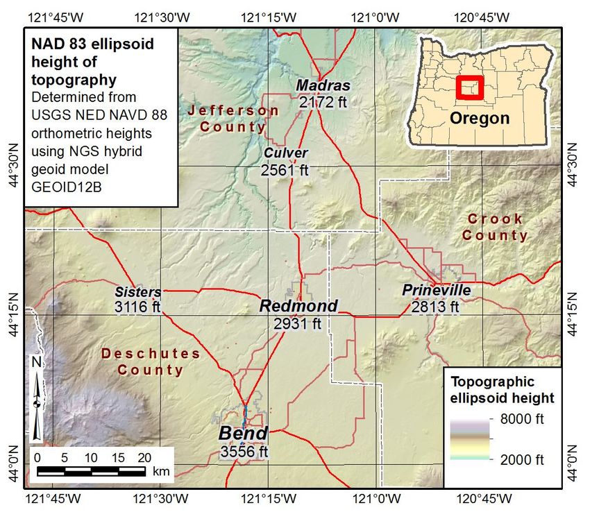
Ground Truth for the Future

Figure 1. Map projection developable surfaces and their projection axes.

For all non-conformal projections (such as equal area projections), meridians and parallels
generally do not intersect at right angles, and scale error varies with direction, so there is no
unique linear distortion at a point. These characteristics make non-conformal projections
inappropriate for most surveying and engineering applications.

The “flat” surface upon which coordinates are projected is called the developable surface. There
are three types – plane, cylinder, and cone – as shown in Figure 1. Each of these is “flat” in the
sense that it can be represented as a plane without distortion, because it has an infinite radius of
curvature in at least one direction. Conceptually, the cylinder and cone can be “cut” parallel to
their central axis (which is the direction of infinite radius of curvature) and laid flat without

 August 2019                                                                                  Page 4

Ground Truth for the Future

changing the relationship between the projected coordinates. Another way to think of it is that
there is only one developable surface, the cone: a cone of infinite height is a cylinder, and a cone
of zero height is a plane.

Each of the projection types listed in Table 1 is usually defined with a set of five or six
parameters (although in some cases an LCC and OM can require seven or eight parameters,
respectively). One is k0, the projection scale (factor) on the projection axis. The projection axis
is the line along which projection scale is minimum and constant with respect to the reference
ellipsoid, as shown in Figure 1. It is the central meridian ( C) for the TM, the central parallel
( C) for the LCC, and the skew axis for the OM. Actually, the scale is not quite constant along
the OM skew axis but is minimum at a single point (the local origin) and increases slowly along
the axis with distance from the origin. The stereographic projection does not have a projection
axis per se but rather a single point of minimum scale at its origin. For the two-parallel LCC, k0
is defined as less than 1 implicitly, by the distance between the north and south standard parallels
(the further apart the standard parallels, the smaller is k0)

The k0 value defines the scale relationship between the ellipsoid and conformal developable
surfaces, as listed below and shown in Figure 2:

   •   k0 < 1. The developable surface is inside (“below”) the ellipsoid and intersects the
       ellipsoid along two curves on either side of the projection axis, beyond which the
       developable surface is outside (“above”) the ellipsoid. In this case the projection is called
       secant because it cuts through the ellipsoid. Secant is the most common projection
       configuration for published PCSs (such as SPCS, UTM, and UPS) because it covers the
       largest region with the least absolute scale error with respect to the ellipsoid. Positive and
       negative scale errors are balanced for secant projection zone as shown in Fig. 2, with
       approximately the middle 71% of the developable surface below the ellipsoid and the
       outer 14.5% on either side above the ellipsoid. The “zone” is the area on the Earth where
       the PCS is used.

   •   k0 = 1. The developable surface is tangent to the ellipsoid. That is, it touches the ellipsoid
       along its projection axis (or at a single point for the Stereographic projection).

   •   k0 > 1. The developable surface is above the ellipsoid and does not intersect the ellipsoid
       surface anywhere. This approach is used to place the developable surface near the
       topographic surface, which is typically above the ellipsoid. The intent is to decrease
       linear distortion of the projected coordinates with respect to the ground surface, rather
       than the ellipsoid surface.

In addition to the projection axis scale, at least four other parameters are needed to fully define
the projections listed in Table 1. Two of these are the latitude and longitude of its geodetic
origin ( 0, 0). The geodetic origin may or may not be located on the projection axis. It is
always on the central meridian of the TM ( 0 = C) but often is not on the central parallel of the
LCC projection ( 0 ≠ C), in which case at least six parameters are required to define an LCC.
The other two parameters are the projected coordinate values of the geodetic origin, often called
the grid origin and specified as false northing (N0) and false easting (E0) in this document. Grid

 August 2019                                                                                 Page 5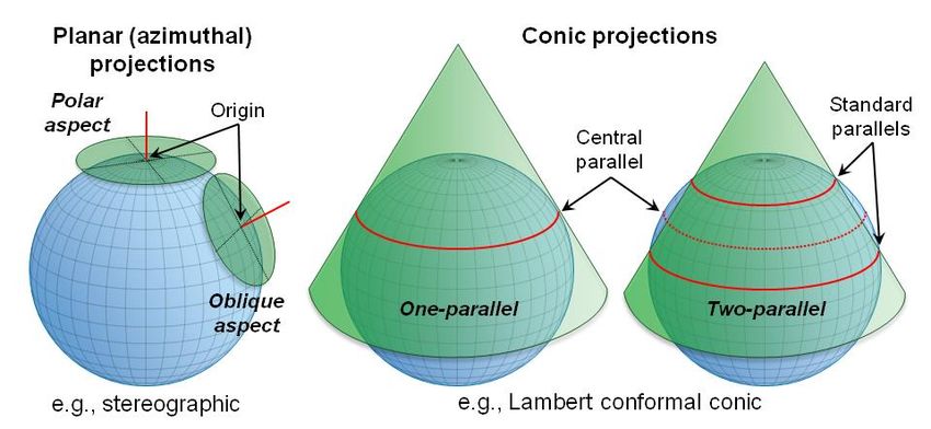
Ground Truth for the Future

origin values are usually selected such that projected coordinates are positive within the zone.
An additional (sixth) parameter called the skew axis azimuth ( 0) is required for the OM
projection to specify the orientation of its skew axis ( 0 can also be specified implicitly by using
a two-point definition).

Figure 2. Secant, tangent, and non-intersecting projection developable surfaces.

Map projection distortion
Map projection distortion is an unavoidable consequence of attempting to represent a curved
surface on a flat surface. It can be thought of as a change in the “true” relationship between
points located on the surface of the Earth and the representation of their relationship on a plane.
Distortion cannot be eliminated — it is a Fact of Life. The best that can be done is to decrease
the effect.
There are two general types of map projection distortion, linear and angular:
1. Linear distortion. Although formally defined infinitesimally at a point, it can be thought of
   as the finite difference in distance between a pair of grid (map) coordinates when compared
   to the true (“ground”) distance, denoted here by δ.
   •   Can express as a ratio of distortion length to ground length:
       ○ E.g., feet of distortion per mile; parts per million (= mm per km)
       ○ Note: 1 foot / mile = 189 ppm = 189 mm / km

 August 2019                                                                                Page 6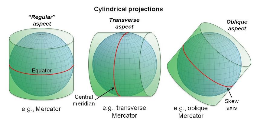
Ground Truth for the Future

   •   Linear distortion can be positive or negative:
       ○ POSITIVE distortion means the projected grid (map) length is LONGER than the
          “true” horizontal (ground) distance.
      ○ NEGATIVE distortion means the projected grid (map) length is SHORTER than the
          “true” horizontal (ground) distance.
2. Angular distortion. For conformal projections, it equals the convergence (mapping) angle, γ.
   The convergence angle is the difference between projected grid (map) north and true
   (geodetic) north – a useful property for surveying applications.
   • Convergence angle is zero on the projection central meridian, positive east of the central
      meridian, and negative west of the central meridian.
   • Magnitude of the convergence angle increases with distance from the central meridian,
      and its rate of change increases with increasing latitude, as shown in Table 2.
   • For the OM projection, there is no true central meridian (i.e., longitude along which the
      convergence angle is zero). However, the meridian passing through the local origin has a
      convergence very close to zero (and is zero at the origin), and the values in this table can
      be used to estimate the convergence angle for the OM local origin.
   • Usually convergence is not as much of a concern as linear distortion, and it can only be
      minimized by staying close to the projection central meridian (or limiting surveying and
      mapping activities to equatorial regions of the Earth). Note that the convergence angle is
      zero everywhere for the regular Mercator projection. Even though this projection is
      conformal, it is not suitable for large-scale mapping in non-equatorial regions due to its
      extreme distortion.

Table 2. Convergence angles at various latitudes, at a distance of 1 mile (1.6 km) east (positive)
and west (negative) of central meridian for TM and projection (and LCC projection with central
parallel equal to latitude in table).
                Convergence                      Convergence                     Convergence
 Latitude                         Latitude                         Latitude
               1 mi from CM                     1 mi from CM                    1 mi from CM
     0°          0° 00’ 00”          30°         ±0° 00’ 30”          60°         ±0° 01’ 30”
     5°         ±0° 00’ 05”          35°         ±0° 00’ 36”          65°         ±0° 01’ 51”
    10°         ±0° 00’ 09”          40°         ±0° 00’ 44”          70°         ±0° 02’ 23”
    15°         ±0° 00’ 14”          45°         ±0° 00’ 52”          75°         ±0° 03’ 14”
    20°         ±0° 00’ 19”          50°         ±0° 01’ 02”          80°         ±0° 04’ 54”
    25°         ±0° 00’ 24”          55°         ±0° 01’ 14”          85°         ±0° 09’ 53”

 August 2019                                                                              Page 7
Ground Truth for the Future

One can think of linear distortion as being due to the projection developable surface (plane, cone,
or cylinder) departing from the reference ellipsoid. No ellipsoidal forms of conformal
projections are perspective. That is, they cannot be created geometrically by constructing
straight lines that radiate from some point and intersect a plane, as implied by Figure 2. But it is
still useful to think of linear distortion increasing as the “distance” of the developable surface
from the ellipsoid increases. In that sense, linear distortion is entirely a function of “height” with
respect to the ellipsoid.

Although total linear distortion is (conceptually) due to departure of the developable surface
from the ellipsoid, it is convenient to separate it into two components: one due to Earth
curvature and one due to height above or below the reference ellipsoid. Indeed, this “total”
distortion is often computed as the product of these two components and called the “combined”
scale error (or factor). The relative magnitude of each at a point of interest depends on its
horizontal distance from the projection axis and its ellipsoid height.

Figure 3 provides a conceptual illustration of distortion as a geometric departure of the
developable surface from the reference ellipsoid. Table 3 gives the range of distortion due to
curvature for various projection zone widths, and Table 4 gives change in distortion due to
change in height, but total distortion is always a combination of both.

Figure 3. Linear distortion of secant map projection with respect to ellipsoid and topography.

 August 2019                                                                                 Page 8

Ground Truth for the Future

Table 3. Maximum range in linear distortion due to Earth curvature for various zone widths
(perpendicular to projection axis).

       Zone width for secant         Maximum range in linear distortion, (δ + 1) = k
    projections (i.e., balanced    Parts per million                         Ratio
 positive and negative distortion)                   Feet per mile
                                      (mm/km)                           (absolute value)
         16 miles (25 km)                    ±1 ppm          ±0.005 ft/mile      1 : 1,000,000
         35 miles (57 km)                    ±5 ppm          ±0.026 ft/mile          1 : 200,000
         50 miles (81 km)                    ±10 ppm         ±0.053 ft/mile          1 : 100,000
         71 miles (114 km)                   ±20 ppm          ±0.11 ft/mile          1 : 50,000
        112 miles (180 km)                   ±50 ppm          ±0.26 ft/mile          1 : 20,000
 ~158 miles (255 km) e.g., SPCS*            ±100 ppm          ±0.53 ft/mile          1 : 10,000
 ~317 miles (510 km) e.g., UTM†             ±400 ppm          ±2.11 ft/mile           1 : 2500
                                   †
*State Plane Coordinate System;        Universal Transverse Mercator

Table 4. Change in projection linear distortion due to change in ellipsoid height.

          Change in                    Change in linear distortion, (δ + 1) = RG / (RG + h)
      ellipsoid height,         Parts per million                                  Ratio
               h                                          Feet per mile
                                   (mm/km)                                    (absolute value)
      ±100 feet (30 m)                  ±4.8 ppm          ±0.025 ft/mile        ~1 : 209,000
      ±400 feet (120 m)                 ±19 ppm            ±0.10 ft/mile         ~1 : 52,000
     ±1000 feet (300 m)                 ±48 ppm            ±0.25 ft/mile         ~1 : 21,000
    +2500 feet (750 m)*                –120 ppm            –0.63 ft/mile             ~1 : 8400
   +3300 feet (1000 m)**               –158 ppm            –0.83 ft/mile             ~1 : 6300
   +14,400 feet (4400 m) †             –690 ppm             –3.6 ft/mile             ~1 : 1450
*Approximate mean topographic ellipsoid height of the conterminous US (CONUS)
** Approximate mean topographic ellipsoid height in CONUS west of 100°W longitude
†
  Approximate maximum topographic ellipsoid height in CONUS

Rules of thumb for ±5 ppm distortion:
• Due to curvature: within ±5 ppm for area 35 miles wide (perpendicular to projection axis).
• Due to change in topographic height: ±5 ppm for range in height of ±100 ft.

 August 2019                                                                                Page 9
Ground Truth for the Future
Methods for creating low-distortion projected coordinate systems
1. Design a Low Distortion Projection (LDP) for a specific geographic area.
Use a conformal projection referenced to the existing geometric reference frame (described
in detail in next section).
2. Scale the reference ellipsoid “to ground”.
A map projection referenced to this new “datum” is then designed for the project area.
Problems: Main one is that method is more complex but performs no better than an LDP.
• Requires a new ellipsoid for every coordinate system. Therefore the five or six
projection parameters plus two ellipsoid parameters are required, for a total of seven or
eight parameters to define each system.
• Coordinates must be transformed to the new ellipsoidal system prior to being projected.
So projection algorithm must include a datum transformation, and this can make these
systems more difficult to implement.
• The transformed latitudes of points can differ substantially from the original values, by
more than 3 feet (1 meter) for heights greater than 1000 ft (300 m). This can cause
incorrect projected coordinates if original geodetic coordinates are not transformed prior
to projecting.
3. Scale an existing published map projection “to ground”.
Referred to as “modified” State Plane when an existing SPCS projection definition is used.
Problems:
• Generates coordinates with values similar to “true” State Plane (can cause confusion).
○ Can eliminate this problem by translating grid coordinates to get smaller values.
• Often yields “messy” parameters when a projection definition is back-calculated from the
scaled coordinates (e.g., to import the data into a GIS).
○ More difficult to implement in a GIS, and may cause problems due to rounding or
truncating of “messy” projection parameters (especially for large coordinate values).
○ Can reduce this problem through judicious selection of “scaling” parameters.
• Does not reduce the convergence angle (it is same as that of original SPCS definition).
Likewise, arc-to-chord correction is the same as original SPCS (used along with
convergence angle for converting grid azimuths to geodetic azimuths).
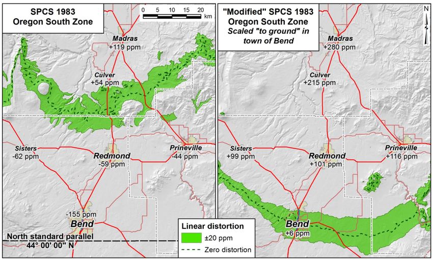
• MOST IMPORTANT: Usually does not minimize distortion over as large an area as
the other two methods.
○ Extent of low-distortion coverage generally decreases as distance from projection axis
increases.
○ State Plane axis usually does not pass through the project area and in addition may be
oriented in a direction that decreases the area of low distortion coverage.
○ Figure 4 illustrates this problem with “modified” SPCS as compared to an LDP.
August 2019 Page 10Ground Truth for the Future (a) Typical SPCS situation (for LCC projection). Projection is secant to ellipsoid, with developable surface below topographic surface. (b) SPCS scaled “to ground” at design location. Central parallel in same location as original SPCS; note developable surface inclined with respect to topographic surface. (c) LDP design. Note central parallel moved north to align developable surface with topographic surface, thereby reducing distortion over a larger region. Figure 4. Comparison of (a) SPCS, (b) “modified” SPCS, and (c) LDP. August 2019 Page 11
Ground Truth for the Future

Six steps illustrating Low Distortion Projection (LDP) design
The design objective is usually to minimize linear distortion over the largest area possible.
These goals are at odds with one another, so LDP design is an optimization problem. It is
important to also realize that the most difficult part is often not technical but psychological.
There is little value in designing an LDP for a region without first getting concurrence and buy-
in from the many stakeholders impacted by the design. This includes surveyors, engineers, GIS
professionals, as well as public and private organizations that make use of geospatial data in the
design area. Getting stakeholders involved early in the process will increase the likelihood that
the LDP will be adopted and actually used.

The following six steps are intended to illustrate commonly encountered situations in LDP
design. These steps are provided to teach the design concepts; in the actual design process some
of these “steps” can be omitted or modified, especially when designing for large areas. But these
steps work well for small areas (< ~30 miles or 50 km wide perpendicular to the projection axis).

1. Define distortion objective for area of interest and determine representative ellipsoid
   height, ho (not elevation)
   NOTE: This is just to get the design process started. Ellipsoid height by itself is unlikely to
   yield the final design scale, except for small areas, due to curvature and/or systematic change
   in topographic height. It is even possible to skip this step entirely, and instead start the
   process with a projection scale of 1 (or some other arbitrary value). However, considering
   height helps illustrate the concepts behind design the process.
   •   A common objective for “low distortion” is ±20 ppm (±0.1 ft/mile), but this may not be
       achievable due to range of topographic height and/or size of design area. The following
       “rules of thumb” can help guide the initial design. However, it may be possible to
       achieve better results than these guidelines indicate, because both height and areal extent
       affect distortion simultaneously, and one can be used to compensate for the other.
       ○ Size of design area. Distortion due to curvature is within ±5 ppm for an area 35
         miles wide. Note that this width is perpendicular to the projection axis (e.g., east-
         west for TM and north-south for LCC projections). The effect is not linear; range of
         distortion due to curvature increases rapidly with increasing zone width and is
         proportional to the square of the zone width, i.e., doubling the zone width increases
         the distortion by about a factor of four (for this ±5 ppm case, doubling zone width to
         70 miles quadruples the distortion range to about ±20 ppm).
       ○ Range in topographic ellipsoid height. Distortion due to change in topographic
         height is about ±5 ppm for a ±100 ft range in height. Note that this is linear for the
         topographic height ranges on Earth. Thus a range of ±400 ft in height corresponds to
         a range of about ±20 ppm distortion.
   •   The average height of an area may not be appropriate (e.g., because of mountains in the
       design area).
       ○ There is usually no need to estimate height to an accuracy of better than about ±20 ft
         (±6 m); this corresponds to about ±1 ppm distortion. In addition, the initial projection
         scale determined using this height will likely be refined later in the design process.

 August 2019                                                                              Page 12
Ground Truth for the Future
2. Choose projection type and place projection axis near centroid of project area
NOTE: This is just to get the design process started. In cases where the topography
generally changes in one direction, offsetting the projection axis can yield substantially better
results. As with step #1, there is no need to spend a lot of effort on this step, since the effect
of the projection type and axis location is evaluated later in the design process.
• Select a well-known and widely used conformal projection, such as the Transverse
Mercator (TM), Lambert Conformal Conic (LCC), or Oblique Mercator (OM).
○ When minimizing distortion, it is not always obvious which projection type to use,
but for small areas (< ~30 miles or ~50 km wide), both the TM and LCC will usually
provide similar and satisfactory results. However, significantly better performance
can be obtained in many cases when a projection is used with its axis perpendicular to
the general topographic slope of the design area (more on this below).
○ In nearly all cases, a two-parallel LCC should not be used for an LDP (but note that
some software may not support a one-parallel LCC). A two-parallel LCC should not
be used because the reason there are two parallels is to make the projection secant to
the ellipsoid (i.e., to make the central parallel scale less than 1). This is at odds with
the usual objective of scaling the projection so that the developable surface is at the
topographic surface, which is typically well above the ellipsoid, particularly in areas
where reduction in distortion is desired. Even for LDP designs that use secant LCC
definitions, it is easier to design an LDP using a one-parallel rather than two-parallel
LCC.
○ The OM projection can be very useful for minimizing distortion over large areas,
especially areas that are elongate in an oblique direction. It can also be useful in
areas where the topographic slope varies gradually and more-or-less uniformly in an
oblique direction. The disadvantage of this projection is that it is more difficult to use
for designs that account for topographic slope, since both the projection skew axis
location and orientation must be simultaneously optimized. Such designs would be
extremely difficult to perform manually but can be optimized using mathematical
methods (such as least squares). There is also more than one version of the OM
projection; the Hotine OM, also called Rectified Skew Orthomorphic (RSO), is the
most common version of the OM used in the U.S.
○ The oblique stereographic projection can also be used, but it is unlikely that it will
perform better than the TM, LCC, or OM projections since it does not curve with the
Earth in any direction. Situations where it would provide the lower distortion than
the other projections would only rarely (if ever) be encountered. In addition, there are
two common versions (“original” and “double” stereographic), but they do not yield
the same coordinates and so care must be taken to ensure the one used for design is
the same used in subsequent applications (coordinates differ by about 1 foot 20 miles
from the projection origin).
○ When choosing a projection, universal commercial software support, although
desirable, is not an essential requirement. In rare cases where third parties must use a
coordinate system based on a projection not supported in their software, it is possible
for them to get on the coordinate system implicitly, for example by using a 2-D best-
August 2019 Page 13Ground Truth for the Future
fit conformal transformation based on LDP coordinates at common points (e.g., the
so-called horizontal “calibration” or “localization” process available in most
commercial GNSS surveying software).
• Placing the projection axis near the design area centroid is often a good first step in the
design process (or, for the OM projection, parallel to the long axis of the design area).
○ In cases where topographic height increases more-or-less uniformly in one direction,
dramatically better performance can be achieved by offsetting the projection axis
from the project centroid. In such cases a projection type should be chosen such that
its projection axis is perpendicular to the topographic slope (e.g., for topography
sloping east-west, a TM projection should be used; for slope north-south, an LCC
projection should be used). The axis is located such that the developable surface best
coincides with the topographic surface (as shown in Figure 4 for an LCC).
○ Often the central meridian of the projection is placed near the east-west “middle” of
the project area in order to minimize convergence angles (i.e., the difference between
geodetic and grid north). The central meridian is the projection axis only for the TM
projection; its location has no effect on linear distortion for the LCC projection.
3. Scale projection axis to the representative ground height, ho
NOTE: This is just to get the design process started. Ellipsoid height by itself is unlikely to
yield the final design scale, except for small areas, due to curvature and/or systematic change
in topographic height. This step can also be skipped by simply starting with k 0 = 1, but the
following provides the concepts (as well as some mathematical information for step #4).
h0
• Compute map projection axis scale factor “at ground”: k 0 = 1 +
RG
○ For TM projection, k 0 is the central meridian scale factor.
○ For one-parallel LCC projection, k 0 is the standard (central) parallel scale factor.
○ For OM projection, k 0 is the scale at the local origin.
a 1 − e2
• RG is the geometric mean radius of curvature, RG =
1 − e 2 sin 2
and = geodetic latitude of point, and for the GRS 80 ellipsoid:
a = semi-major axis = 6,378,137 m (exact) = 20,925,646.325 international ft
= 20,925,604.474 US survey ft
e2 = first eccentricity squared = f (2 – f ) = 0.00669438002290
f = geometric flattening = 1 / 298.257222101
○ Alternatively, can initially approximate RG using Table 5, since k 0 will likely be
refined in Step #4:
August 2019 Page 14Ground Truth for the Future
Table 5. Geometric mean radius of curvature at various latitudes for the GRS 80 ellipsoid
(rounded to nearest 1000 feet and meters).
Lat feet (meters) Lat feet (meters) Lat feet (meters)
0° 20,855,000 (6,357,000) 35° 20,902,000 (6,371,000) 65° 20,971,000 (6,392,000)
10° 20,860,000 (6,358,000) 40° 20,913,000 (6,374,000) 70° 20,980,000 (6,395,000)
15° 20,865,000 (6,360,000) 45° 20,926,000 (6,378,000) 75° 20,987,000 (6,397,000)
20° 20,872,000 (6,362,000) 50° 20,938,000 (6,382,000) 80° 20,992,000 (6,398,000)
25° 20,880,000 (6,364,000) 55° 20,950,000 (6,385,000) 85° 20,995,000 (6,399,000)
30° 20,890,000 (6,367,000) 60° 20,961,000 (6,389,000) 90° 20,996,000 (6,400,000)
4. Compute distortion throughout project area and refine design parameters
RG
• Distortion computed at a point (at ellipsoid height h) as = k − 1
RG + h
○ Where k = projection grid point scale factor (i.e., distortion with respect to the
ellipsoid at a point). Note that computation of k is rather involved, and is often done
in commercial software. However, if your software does not compute k, or if you
want to check the accuracy of k computed by your software, equations for doing so
for the TM and LCC projections are provided in section “Projection grid scale factor
and convergence angle computation” later in this document.
○ Multiply by 1,000,000 to get distortion in parts per million (ppm).
• Best approach is to compute distortion over entire area and generate a distortion map and
compute distortion statistics (this helps ensures low-distortion coverage is achieved
where it is desired).
○ Often requires repeated evaluation using different k 0 values and different projection
axis locations.
○ May also warrant trying different projection types.
• General approach for computational refinement:
○ Compute distortion statistics, such as mean, range, and standard deviation for all
points in the design rea.
○ Changing the projection scale only affects the mean distortion; it has essentially no
effect on the variability (standard deviation and range).
○ The only way to reduce distortion variability is by moving the projection axis and/or
changing the projection type. The usual objective is to minimize the distortion range.
Once this is done, the scale can be changed so that the mean distortion is near zero
(this will have no effect on the distortion range or standard deviation).
August 2019 Page 15Ground Truth for the Future
○ Finally, check to ensure the desired distortion is achieved in important areas, and
check to ensure overall performance is satisfactory, by using a map showing
distortion everywhere in the design area. It may be worthwhile to give greater weight
to distortion in populated areas (such as cities), rather than using the same weight for
all areas.
5. Keep the definition SIMPLE and CLEAN!
• Define k 0 to no more than SIX decimal places, e.g., 1.000175 (exact).
○ Note: A change of one unit in the sixth decimal place (±1 ppm) equals distortion
caused by a 20 ft (6 m) change in height.
○ For large areas with variable relief, scale defined to five decimal places (±10 ppm) is
often sufficient.
• Define the central meridian and latitude of grid origin to nearest whole arc-minute.
Using arc minutes evenly divisible by 3 will result in exact values in decimal degrees
(e.g., 121°33’00” W = −121.55°), although some prefer using the nearest 5 arc minutes
(as done for State Plane 1983 and 1927).
• Define grid origin using whole values. Often it is desired to use values with as few digits
as possible (e.g., false easting = 50,000 for a system with maximum easting coordinate
value < 100,000), although there are many different options for selecting values. Note
that the grid origin definition has no effect whatsoever on map projection distortion.
○ It is strongly recommended that the coordinate values everywhere in the design area
be distinct from other coordinate system values for that area (such as State Plane and
UTM) in order to reduce the risk of confusing the LDP with other systems. For
multi-zone LDPs, it could similarly be helpful to keep coordinates between the zones
distinct, if possible.
○ It may be desirable to define grid origins such that the northings and eastings do not
equal one another anywhere in the design area.
○ In some applications, there may be an advantage to using other criteria for defining
the grid origin. For example, it may be desirable for all coordinates in the design area
to have the same number of digits (such as six digits, i.e., between 100,000 and
999,999). In other cases it may be useful to make the coordinates distinct from State
Plane by using larger rather than smaller coordinates, especially if the LDP covers a
very large area. In multi-zone systems, it may also be helpful to define grid origins
such that the values correlate to zone numbers (e.g., coordinates between 3,000,000
3,999,999 m for a zone designated as #3). This approach was used for the Iowa and
Kansas Regional Coordinate Systems (Dennis et al., 2014 and Dennis, 2017b).
6. Explicitly define linear unit and geometric reference system (i.e., geodetic datum)
• Linear unit, e.g., meter (or international foot, or US survey foot, or…?)
○ Although the U.S. survey foot is currently used for SPCS 83 in most states, that linear
unit will be officially deprecated by the U.S. government on December 31, 2022.
August 2019 Page 16Ground Truth for the Future
That means the U.S. survey foot cannot be used for projection definitions that will
become part of the State Plane Coordinate System of 2022, and it will not be
supported by NGS for any component of the National Spatial Reference System
(NSRS) after 2022. However, the U.S. survey foot will continue to be supported as a
legacy unit by NGS in applications that compute State Plane coordinates for zones
where it was officially specified for SPCS 83, and for all zones of SPCS 27.
○ The foot definition used after 2022 will be simply be called the “foot”, and it will be
numerically identical to the foot definition presently called the “international foot”
(i.e., 1 foot = 0.3048 meter exactly). The intent is to have a single, uniform definition
of the foot used throughout the U.S. for all applications
• Geometric reference system (datum), e.g., North American Datum of 1983 (NAD 83)
○ The reference system realization (“datum tag”) and epoch date (e.g., 2010.00) should
not be included in the coordinate system definition (just as it is not included in State
Plane definitions). However, the datum tag and epochs are essential components for
defining the spatial data used within the coordinate system (as shown in a metadata
example later in this document). For NAD 83, the NGS convention is to give the
datum tag in parentheses after the datum name, usually as the year in which the datum
was “realized” as part of a network adjustment. Epoch dates are given after the
datum tag and are preceded by the word “epoch.” Although given as decimal years,
they are usually not the same as the datum tag. Common datum tags and epochs for
NGS control are listed below. Prior to the NAD 83 (2011) epoch 2010.00 realization,
epochs were only used for tectonically active areas and CORS. But that they will be
used for all components of the NSRS after 2022. Below are some common datum
tags and epochs for geometric (“horizontal”) geodetic control:
▪ “2011” for the current NAD 83 (2011) epoch 2010.00 realization, which is
referenced to the North America tectonic plate. A tag of “PA11” is used for
control referenced to the Pacific plate (e.g., Hawaii, American Samoa), and a tag
of “MA11” is used for control referenced to the Pacific plate (e.g., Guam).
▪ “2007” for the (superseded) NSRS2007 (National Spatial Reference System of
2007) realization. Functionally equivalent to the superseded “CORS” datum tag
and referenced to an epoch of 2002.00 for most of the coterminous US and the
Caribbean (an epoch of 2007.00 was used for the western states of AK, AZ, CA,
NV, OR, and WA).
▪ “199x” for most of the various superseded HARN (or HPGN) and Federal Base
Network (FBN) realizations, where x is the last digit of the year of the adjustment
(usually done for a particular state). HARN is “High Accuracy Reference
Network” and HPGN is “High Precision Geodetic Network”.
• Note regarding the State Plane Coordinate System of 2022 (SPCS2022): NGS will
replace NAD 83 with new terrestrial reference frames (TRFs) in 2022. The one for North
America will be called the North American Terrestrial Reference Frame of 2022
(NATRF2022); there will also be a TRF for the Caribbean, Pacific, and Mariana tectonic
plates. The GRS 80 ellipsoid will continue to be used for the SPCS2022. In North
America, horizontal coordinates will change by less than 2 m (6.5 ft). Ellipsoid heights
August 2019 Page 17Ground Truth for the Future
will change by less than ±2 m everywhere. A change in height of 2 m will change linear
distortion by 0.3 ppm. Since the change to the 2022 TRFs will have negligible impact on
the distortion of LDPs designed with respect to NAD 83, those LDPs could continue to
be used with the 2022 datum. However, to avoid confusion it would be prudent to
change the grid coordinates so that LDP coordinates based on the 2022 datum are
significantly different from those referenced to NAD 83. Such a change will not affect
distortion but would reduce the risk of accidentally referencing the wrong datum.
NGS is currently in the process of defining SPCS2022. The references section of this
document includes recently released NGS documents about SPCS2022:
○ A report on the history, status, and possible future of State Plane (Dennis, 2018).
○ New SPCS2022 policy and procedures (NGS, 2019a and 2019b, respectively), which
allow for the use of LDPs for SPCS2022 zones. However, the LDPs must be defined
by the states where they will be used (NGS will not design zone with a distortion
design criterion of less than ±50 ppm, due to lack of resources).
• Note regarding the relationship between NAD 83 and WGS 84: For the purposes of
entering the LDP projection parameters into vendor software, the datum should be
defined as NAD 83 (which uses the GRS 80 reference ellipsoid for all realizations).
Some commercial software implementations assume there is no transformation between
WGS 84 and NAD 83 (i.e., all transformation parameters are zero). Other
implementations use a non-zero transformation, and in some cases both types are
available. The type of transformation used will depend on specific circumstances,
although often the zero transformation is the appropriate choice (even though it is not
technically correct). Check with software technical support to ensure the appropriate
transformation is being used for your application. Additional information about WGS 84
is available from the National Geospatial-Intelligence Agency (NGA, 2014b).
• Note regarding the vertical component of a coordinate system definition: The vertical
reference system (datum) is an essential part of a three-dimensional coordinate system
definition. But LDPs are restricted exclusively to horizontal coordinates. Although the
vertical component is essential for most applications, it is not part of an LDP and must be
defined separately. It should be specified as part of the overall coordinate system
metadata (as shown in the metadata example later in this document). A complete three-
dimensional coordinate system definition must include a vertical “height” component.
Typically the vertical part consists of ellipsoid heights relative to NAD 83 (when using
GNSS) and/or orthometric heights (“elevations”) relative to the North American Vertical
Datum of 1988 (NAVD 88). These two types of heights are related (at least in part) by a
hybrid geoid model, such as GEOID12B, and often a vertical adjustment or
transformation to match local vertical control for a project. The approach used for the
vertical component usually varies from project to project and requires professional
judgment to ensure it is defined correctly. Providing such instructions is beyond the
scope of this document.
August 2019 Page 18Ground Truth for the Future
Design example for a Low Distortion Projection (LDP)
The LDP design example is for the southern Deschutes River valley of central Oregon (shown in
Figure 5). This example follows the design of the Bend-Redmond-Prineville zone in the Oregon
Coordinate Reference System (OCRS). The design process is illustrated in the six steps below.
• First three steps are mainly to initiate the design; step 4 is where the design is optimized
to minimize distortion over the largest area possible.
• Overall design objective is ±20 ppm for the region and ±10 ppm within the three largest
towns (Bend, Redmond, and Prineville).
• Towns of Sisters, Culver, and Madras are also used for evaluation.
Figure 5. LDP design area, showing topographic ellipsoid heights of towns.
August 2019 Page 19Ground Truth for the Future
1. Define distortion objective for area of interest and determine representative ellipsoid
height, ho (not elevation)
To get the process started, ellipsoid heights were obtained at arbitrary locations in each of the
six towns using NAVD 88 orthometric heights from the USGS 1-arcsecond 3DEP dataset
(formerly the National Elevation Dataset) with GEOID12B hybrid geoid heights. These
values are given in Table 6, for a mean topographic ellipsoid height of h0 = 2858 ft
(“representative” value for initial design).
Size of design area. The overall design area is about 45 miles long north-south, and about 35
miles wide east-west. Based on ±10 ppm distortion for a zone width of 50 miles in Table 3,
it appears the design distortion can be achieved, at least with respect to Earth curvature.
Range in topographic ellipsoid height. The height range in Table 6 is 1384 ft (i.e., ±692 ft),
which corresponds to about ±33 ppm based on ±4.8 ppm per ±100 ft in Table 4 — not an
encouraging observation, considering the design objectives of ±20 ppm overall and
especially of ±10 ppm in Bend, Redmond, and Prineville.
Table 6. The six locations (towns) in the project region used to perform LDP design.
Topographic height at location (feet)
NAD 83 NAD 83
Location NAVD 88 GEOID12B NAD 83
latitude longitude
orthometric hybrid geoid ellipsoid
Bend 44°03'29"N 121°18'55"W 3625 -68.8 3556
Redmond 44°16'21"N 121°10'26"W 3000 -69.5 2931
Prineville 44°17'59"N 120°50'04"W 2880 -67.5 2813
Sisters 44°17'27"N 121°32'57"W 3186 -70.1 3116
Culver 44°31'32"N 121°12'47"W 2631 -69.8 2561
Madras 44°38'00"N 121°07'46"W 2242 -70.0 2172
Mean 2927 -69.3 2858
Range 1383 2.6 1384
Std deviation ±473 ±1.0 ±473
2. Choose projection type and place projection axis near centroid of project area
Upon initial inspection, it is not clear which projection type would be best, so we will
evaluate both TM and LCC. To get the process started, the projection axes placed near the
center of the region.
For the TM projection, the initial central meridian is set at λ0 = 121° 15’ 00” W.
For the LCC projection, the initial central parallel is set at φ 0 = 44° 20’ 00” N.
August 2019 Page 20Ground Truth for the Future
Because the design area is somewhat longer north-south than east-west (45 vs. 35 miles), the
TM projection may be the better choice. On the other hand, the topographic height overall
decreases from north to south, which tends to favor the LCC projection. The performance of
these projections will be evaluated as part of the design process.
3. Scale projection axis to representative ground height, ho
First compute Earth radius at mid-latitude of φ = 44° 20’ 00” N (same as central parallel for
initial LCC design):
a 1 − e2 20,925,646.325 1 − 0.006694380023
RG = = = 20,923,900 ift
1 − e sin 1 − 0.006694380023 sin (44.333333) 2
2 2
Thus the central meridian scale factor scaled to the representative ellipsoid height is
h0 2858
k0 = 1 + =1+ = 1.00014 (rounded to five decimal places)
RG 20,923,900
Based on these results, the following initial TM and LCC projections are defined (will check
and refine as necessary in step #4). Only the characteristics affecting distortion need to be
specified at this point. Other parameters, such as false northings and eastings, will be
specified after a design is selected based on distortion performance.
Projection: Transverse Mercator Lambert Conformal Conic
Projection axis: λ0 = 121° 15’ 00” W φ0 = 44° 20’ 00” N
Projection axis scale: k0 = 1.00014 k0 = 1.00014
4. Compute distortion throughout project area and refine design parameters
Distortion can also be computed at discrete points. These points can be NGS control points,
other surveyed points, or any point with a reasonable accurate topographic ellipsoid height.
For this design example, the heights at the given location for each of the six towns are used,
which are accurate to about ±10 ft (corresponding to distortion accuracy of ±0.5 ppm). A
computation example for each of the two initial LDP designs is provided for the point
representing the town of Bend using the values from Table 6:
Bend: φ = 44° 03’ 29” N, λ = 121° 18’ 55” W, h = 3556 ft,
RG
where linear distortion is computed as = k − 1
RG + h
a 1 − e2
and geometric mean radius of curvature as RG = = 20,923,218 ift.
1 − e 2 sin 2
August 2019 Page 21Ground Truth for the Future
The value of k can be computed using various geospatial software packages. If such software
is not available, it can be computed using the equations given later in this document. The
value obtained for the TM is k = 1.000 140 336, and for the LCC is k = 1.000 151 486.
Using these values gives the following values of distortion at the point in Bend:
20,923,218
TM: = 1.000140336 − 1 = 0.999 970 387 – 1 = –29.6 ppm
20,923,218 + 3556
20,923,218
LCC: = 1.000151486 − 1 = 0.999 981 534 – 1 = –18.5 ppm
20,923,218 + 3556
Despite using the mean topographic height of the six towns for determining the projection
scale, the distortion magnitude for both projections exceeds the ±10 ppm criterion for Bend.
This could be fixed for the point in Bend by increasing the projection scale by, say, 20 ppm
to k0 = 1.00016, which would change the values to –9.6 ppm and +1.5 ppm for the TM and
LCC projections, respectively. However, this would also increase the distortion at the other
points by 20 ppm, yielding a maximum in Madras of +57.3 ppm and +69.9 ppm for the TM
and LCC projections, respectively. Such distortion is much too large, so a different approach
is needed.
For a given projection, variability can only be changed by changing the location of the
projection axis. In this case, simply changing the projection scale alone will not achieve the
desired result. Changing their locations will change the variability of the distortion in the
design area. We can assess the variability by the distortion range and standard deviation.
The results of doing that for the TM and LCC projections are shown in tables 7 and 8,
respectively. In addition to changing the projection axis locations, in all design alternatives
the axis scale was also changed so that the mean distortion was within ±10 ppm.
As shown in Table 7, the distortion standard deviation and range of the TM design
alternatives both decrease as the projection axis (central meridian) location is moved east,
with a minimum range of 49.5 ppm at λ0 = 120° 40’ W. However, the changes are generally
modest, with no substantial improvement from the initial design.
In contrast, Table 8 shows that the change in distortion standard deviation and range of the
LCC design alternatives is significant as the projection axis (central parallel) location is
changed. The standard deviation and range decrease from ±24.6 and 68.3 from the initial
design to a minimum of ±7.6 ppm and 19.4 ppm (for φ0 = 44° 45’ N).
August 2019 Page 22Ground Truth for the Future
Table 7. Distortion performance for six different TM projection alternatives (initial design
values are italicized).
Initial
TM axis scale 1.00013 1.00013 1.00012 1.00011 1.00010
1.00014
TM axis longitude 121°15'W 121°10'W 121°00'W 120°45'W 120°40'W 120°35'W
Location Linear distortion for TM projection (parts per million)
Bend -29.6 -38.2 -32.1 -24.7 -26.7 -27.7
Redmond 0.4 -10.1 -7.7 -6.0 -9.9 -12.7
Prineville 19.1 4.2 -2.3 -13.9 -22.2 -29.5
Sisters -1.9 -7.5 4.7 21.1 22.1 24.1
Culver 17.7 7.8 11.1 14.3 10.8 8.4
Madras 37.3 26.3 27.5 27.3 22.8 19.3
Mean 7.2 -2.9 0.2 3.0 -0.5 -3.0
Range 66.9 64.5 59.6 52.1 49.5 53.6
Std deviation ±23.0 ±21.6 ±20.0 ±20.9 ±22.0 ±23.5
Table 8. Distortion performance for six different LCC projection alternatives (initial design
values are italicized; final values are bold).
Initial Final
LCC axis scale 1.00013 1.00012 1.00011 1.00010
1.00014 1.00012
LCC axis latitude 44°20'N 44°30'N 44°35'N 44°40'N 44°45'N 44°50'N
Location Linear distortion (parts per million)
Bend -18.5 -10.4 -8.2 6.1 12.4 20.9
Redmond 0.5 -2.2 -5.4 3.5 4.4 7.5
Prineville 5.7 1.7 -2.2 6.0 6.3 8.7
Sisters -8.6 -12.3 -16.0 -7.5 -7.0 -4.4
Culver 23.2 7.7 -1.9 0.6 -4.8 -8.0
Madras 49.9 28.9 16.6 16.4 8.3 2.3
Mean 8.7 2.2 -2.9 4.2 3.3 4.5
Range 68.3 41.2 32.5 23.9 19.4 28.9
Std deviation ±24.6 ±15.0 ±10.8 ±7.8 ±7.6 ±10.4
August 2019 Page 23Ground Truth for the Future
Although the standard deviation and range are minimum for φ0 = 44° 45’ N, the distortion
was becoming excessive in the southern end of the design region, as exemplified by the
distortion of +12.4 ppm in Bend. For this case, the central parallel is far enough north that
distortion in the southern part of the design area was changing too rapidly with change in
latitude. Because of this affect, as well as inspection of performance in other areas of the
design region (as shown on the distortion maps), a design with φ0 = 44° 40’ N and k0 =
1.00012 was selected for the final design (values in bold in Table 8). This design has
distortion less than 10 ppm in Bend, Redmond, and Prineville, and variability is also less for
these towns.
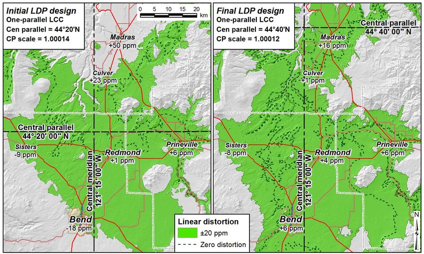
Evaluating distortion values at discrete points is typically not sufficient for optimizing an
LDP design. A more comprehensive evaluation can be done by computing distortion on a
regular grid. Distortion can then be visualized and analyzed everywhere, as shown in the
map in Figure 6 for the final LDP design. The area with ±20 ppm distortion is also shown in
Figure 7, for both the initial and final LCC designs. Note the improvement in low-distortion
coverage gained by moving the central parallel north rather than leaving it at the center of the
design area.
5. Keep the definition SIMPLE and CLEAN!
The LCC projection parameters affecting distortion were defined in the previous step and are
given again in this step, along with the other needed parameters that do NOT affect linear
distortion.
• LCC ko defined to exactly FIVE decimal places: k0 = 1.00012 (exact)
• Both central parallel and central meridian are defined to nearest whole arc-minute. .
φ0 = 44° 40’ 00” N = 31.666666666667° and λ0 = 121° 15’ 00” W = −121.25°
The central meridian (λ0) was selected as a clean value near the east-west center of the
design area (has no effect on distortion).
For an LCC projection, the latitude of grid origin must also be specified; it is the latitude
where the false northing is defined (i.e., the northing on the central meridian at that
latitude). It also has no effect on distortion, and it was set equal to the central parallel.
This was done for simplicity and consistency, so that the LCC projection is defined with
five parameters, same as the number of parameters used for a TM projection.
• Grid origin is defined using clean whole values with as few digits as possible:
N0 = 130,000.000 m and E0 = 80,000.000 m
Metric values were used to avoid confusion between international and US survey feet in
the defined parameters (as also done in Oregon State Plane). These values were selected
to keep grid coordinates positive but as small as possible throughout the design area (and
also distinct from State Plane and UTM coordinates).
August 2019 Page 24You can also read