Guided accumulation of active particles by topological design of a second-order skin effect
←
→
Page content transcription
If your browser does not render page correctly, please read the page content below
Guided accumulation of active particles by topological design of a second-order skin effect

                                                                                      Lucas S. Palacios,1 Serguei Tchoumakov,2 Maria Guix,1 Ignacio
                                                                                    Pagonabarraga,3, 4, 5 Samuel Sánchez∗ ,1, 6, ∗ and Adolfo G. Grushin∗2, †
                                                                                      1
                                                                                        Institute for Bioengineering of Catalonia (IBEC), Barcelona Institute for
                                                                                  Science and Technology (BIST), Baldiri I Reixac 10-12, 08028 Barcelona, Spain
                                                                               2
                                                                                 Univ. Grenoble Alpes, CNRS, Grenoble INP, Institut Néel, 38000 Grenoble, France
                                                          3
                                                            Departament de Física de la Matèria Condensada, Universitat de Barcelona, C. Martí Franquès 1, 08028 Barcelona, Spain
                                                               4
                                                                 University of Barcelona Institute of Complex Systems (UBICS), Universitat de Barcelona, 08028 Barcelona, Spain
                                                                                            5
                                                                                              CECAM, Centre Européen de Calcul Atomique et Moléculaire,
                                                                   École Polytechnique Fédérale de Lausanne (EPFL), Batochime, Avenue Forel 2, 1015 Lausanne, Switzerland
                                                                 6
                                                                   Institució Catalana de Recerca i Estudis Avançats (ICREA), Pg. Lluís Companys 23, 08010 Barcelona, Spain.
                                                                                                                  (Dated: July 14, 2021)
arXiv:2012.14496v2 [cond-mat.soft] 13 Jul 2021

                                                                                   ABSTRACT                                  The recent discovery that topological properties emerge
                                                                                                                          in the class of out-of-equilibrium systems described by non-
                                                    Collective guidance of out-of-equilibrium systems with-               Hermitian matrices, which includes active matter systems [5],
                                                 out using external fields is a challenge of paramount im-                has opened the possibility to engineer robust behaviour out of
                                                 portance in active matter, ranging from bacterial colonies               equilibrium [6, 7]. While in equilibrium topological boundary
                                                 to swarms of self-propelled particles. Designing strate-                 states are predicted by a non-zero bulk topological invari-
                                                 gies to guide active matter and exploiting enhanced dif-                 ant, a feature known as the bulk-boundary correspondence,
                                                 fusion associated to its motion will provide insights for                in non-Hermitian systems, this correspondence is broken by
                                                 application from sensing, drug delivery to water remedia-                the skin-effect [8–13]. For example, in a one-dimensional
                                                 tion. However, achieving directed motion without breaking                (1D) chain of hopping particles, the first-order non-Hermitian
                                                 detailed balance, for example by asymmetric topographi-                  skin effect arises from the asymmetry between left and right
                                                 cal patterning, is challenging. Here we engineer a two-                  hopping probabilities, which results in an accumulation of a
                                                 dimensional periodic topographical design with detailed                  macroscopic number of modes, of the order of the system size,
                                                 balance in its unit cell where we observe spontaneous                    on one side of the system. This 1D effect occurs in systems
                                                 particle edge guidance and corner accumulation of self-                  without an inversion center, and has been observed in pho-
                                                 propelled particles. This emergent behaviour is guaran-                  ton dynamics [14], mechanical metamaterials [15–17], optical
                                                 teed by a second-order non-Hermitian skin effect, a topo-                fibers [18] and topoelectrical circuits [19, 20]. In 1D, the skin-
                                                 logically robust non-equilibrium phenomenon, that we use                 effect occurs if a topological invariant, the integer associated
                                                 to dynamically break detailed balance. Our stochastic cir-               to the winding of the complex spectrum of the normal modes,
                                                 cuit model predicts, without fitting parameters, how guid-               is non-zero [10, 21, 23].
                                                 ance and accumulation can be controlled and enhanced                         Higher-dimensional versions of the skin effect can dis-
                                                 by design: a device guides particles more efficiently if the             play a considerably richer and subtle phenomenology [6, 11–
                                                 topological invariant characterizing it is non-zero. Our                 14, 24–29, 31, 36] In this work we are interested in an elu-
                                                 work establishes a fruitful bridge between active and topo-              sive second-order non-Hermitian skin effect, predicted only
                                                 logical matter, and our design principles offer a blueprint              in out-of-equilibrium systems in two dimensions (2D) [6, 11–
                                                 to design devices that display spontaneous, robust and pre-              14, 31]. It differs from the first-order skin effect because (i)
                                                 dictable guided motion and accumulation, guaranteed by                   it can occur in inversion symmetric systems, accumulating
                                                 out-of-equilibrium topology.                                             modes at opposing corners rather than edges [20, 37], and (ii)
                                                                                                                          the number of accumulated modes is of order of the system
                                                                                                                          boundary L, rather than its area L2 . While the first-order
                                                                            INTRODUCTION                                  non-Hermitian skin effect requires inversion to be broken, e.g.
                                                                                                                          due to an applied field, the emergence of the second-order
                                                    The last decades of research in condensed matter physics              non-Hermitian skin effect is guaranteed by the presence of
                                                 have revealed that exceptionally robust electronic motion oc-            certain symmetries [6, 13]. However, predicting the second-
                                                 curs at the boundaries of a class of insulators known as topo-           order non-Hermitian skin effect is challenging in general, and
                                                 logical insulators [1, 2]. These ideas extend beyond solid-state         it remains unobserved. Dissipation, which drives a system out
                                                 physics, and predict guided boundary motion in systems in-               of equilibrium, is hard to control experimentally in quantum
                                                 cluding photonic [3], acoustic and mechanical systems [4].               electronic devices, therefore calling for platforms to realize the
                                                                                                                          second-order non-Hermitian skin effect.
                                                                                                                            Active matter systems [38] are a natural platform to explore
                                                                                                                          non-Hermitian topological physics, since these systems absorb
                                                 ∗   ssanchez@ibecbarcelona.eu                                            and dissipate energy [5]. Often, the hydrodynamic equations
                                                 †   adolfo.grushin@neel.cnrs.fr                                          that describes their flow can be mapped to a topological Hamil-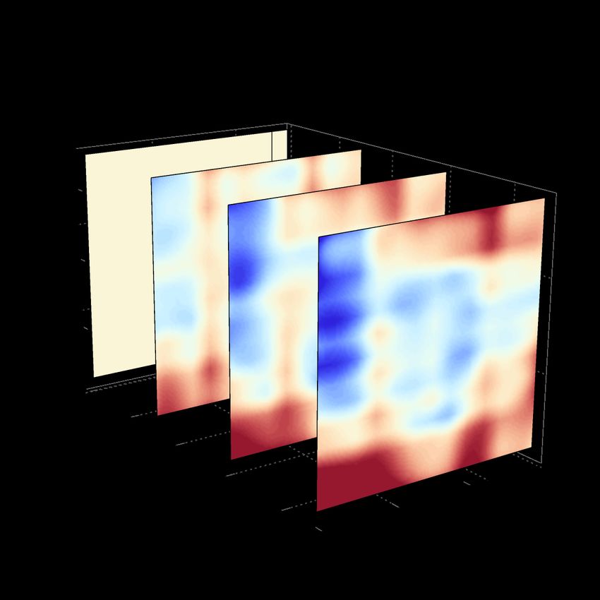
2

a                                                                          b

                           trivial                                                                                   topological
            unit cell                                                                                      unit cell

c                                          d                                                       e
         mask                                          Pt


                        microscope


                        and camera
 f                                                 g                                                   h

     P                                                 P                                                     P

           initial synchronized                             post-selected corner                                       post-selected uniform

Figure 1. Experimental designs. a and b show the trivial and the topological devices respectively, with (Lx , Ly ) = (13, 14) unit cells. The
insets depict the unit cells which are the same for both devices except the vertical wide and narrow channels are reversed, as shown in the
zoomed central inset and emphasized with orange and purple lines. The topological device displays chiral edge modes at the top and bottom,
sketched in blue and red respectively, and which are related to a non-vanishing Hermitian topological invariant, wH . These topological edge
modes have a non-vanishing non-Hermitian winding number, wnH , responsible for the accumulation of active particles at the corners. This
accumulation at the corners is expected to vanish for the trivial device, see the uniform density in green, because the topological invariant
ν = wH wnH vanishes. c and d show a schematic of the experimental set up, where Pt-coated SiO2 Janus particles self-propel when hydrogen
peroxide is added, following the topographic features of each design. e shows a portion of the device to illustrate the tracking of particles by
using a neural network, each particle is uniquely identified within our algorithm. We locate particles within the cells outlined by the dashed
lines. f-h show the probability distribution data, P, of particles on the lattice when trajectories are tracked and synchronized to start at the same
initial time f, post-selected to start at opposing corners g, or post-selected to have an initial uniform distribution h. The particle distributions in
g and h are shown three minutes after synchronization. These initial particle distributions are similar for both topological and trivial devices.

tonian. This strategy predicts topologically protected motion                  tally in active nematic cells [43], and robotic [16] and piezo-
of topological waves in active-liquid metamaterials [39–41],                   electric metamaterials [17].
skin-modes in active elastic media [37], and emergent chiral
behaviour for periodic arrays of defects [42]. Non-Hermitian                      In this work we design microfabricated devices [44–46]
topology in active matter has been demonstrated experimen-                     that display a controllable second-order non-Hermitian skin
                                                                               effect (see Fig. 1). These devices are designed to satisfy de-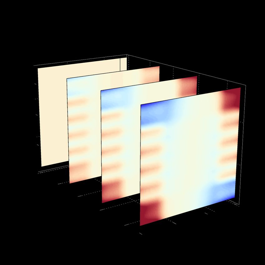
3

tailed balance on their unit cell, such that the flow of particles    the initial particle distribution. We overcome this limitation by
through a unit cell vanishes. The non-Hermitian skin effect           post-selecting trajectories so that they start either from the top
dynamically breaks this detailed balance on the top and bottom        left and bottom right cells (Fig. 1g), or from a uniform distri-
edges, and we use it to guide and accumulate self-propelled           bution over all cells (Fig. 1h). This post-selection is possible
Janus particles. In contrast to hydrodynamic descriptions, the        due to our tracking system, and it is a differentiating aspect
topological particle dynamics in our devices is quantitatively        between active particle and electronic systems.
described by a stochastic circuit model [47] without fitting             We study devices built out of (Lx , Ly ) = (12, 6) and (Lx , Ly )
parameters. It establishes that topological circuits, where a         = (13, 14) unit-cells in the horizontal (x) and vertical (y) direc-
topological invariant ν = 1, display the second-order non-            tions, with either a small or a large density of injected active
Hermitian skin effect that guides and accumulates particles           particles (see Methods). In the main text, we focus on the larger
more efficiently than the topologically trivial circuits, with        device, with (Lx , Ly ) = (13, 14), see Fig. 1. All other devices
ν = 0. This phenomenon occurs without external stimuli, e.g.          and the corresponding results are shown in the Supplementary
electrical or magnetic fields, a useful feature for active matter     Discussion 2.
applications [38, 48, 49], and to extend our design principles           Because of the irregular microchannel walls and the col-
to metamaterial platforms [3, 4, 50].                                 lisions between particles, we model the collective motion of
                                                                      active particles as a Brownian motion in a stochastic network
                                                                      with transition probabilities between the cells introduced in
                            RESULTS                                   Fig. 1e. Cells are represented by nodes in our model, depicted
                                                                      in Figs. 2a,b. Neglecting correlations between particles due
       Coupled-wire device design and stochastic model                to collisions, that we refer to as jamming, the continuous-time
                                                                      Markov master equation governs the probability distribution
   Our design realizes the coupled-wire construction, a theo-         of the particles in time as [47]
retical tool to construct topological phases [2]. This is possible
                                                                                                   ∂P
by the precise engineering of microchannel devices (see Meth-                                  τ      = Ŵ · P,                        (1)
ods) [44]. Each device contains two types of horizontal mi-                                        dt
crochannels, the wires, which are coupled vertically, forming         where P = Pijσ is the probability to observe a particle on site
a 2D mask (see Fig. 1a, b). The horizontal microchannels are          (σ, i, j), σ ∈ {A, B} is the sub-cell index and (i, j) are the
consecutive left or right oriented hearth-shaped ratchets, that       primitive-cell indices (see Figs. 2a and b). τ is the timescale for
favour a unidirectional motion towards their tip [46]. Their
                                                                      a particle to move between adjacent sites. Ŵ is the transition
left-right orientation alternates vertically. These horizontal
                                                                      rate matrix (written explicitly in the Supplementary Discus-
microchannels are coupled by vertical microchannels that are
                                                                      sion 1). It depends on the four transitions probabilities: t±
straight, designed to imprint a symmetric vertical motion to the
                                                                      for the motion along or against the ratchet-like microchan-
nanoparticles. The vertical microchannels alternate in width,
                                                                      nels and, t1 and t2 for the motion along the wide and narrow
with successive narrow and wide channels. Wide channels are
                                                                      microchannels, respectively. The time scale τ and the condi-
more likely to be followed by the active particles than narrow
                                                                      tional probabilities are extracted from our experimental data
channels.
                                                                      in Supplementary Discussion 1. τ is roughly ten seconds
   Using these principles, we design two types of devices that        and since it depends on various factors, from the concentra-
we coin trivial and topological, depicted in Figs. 1a and b,          tion of chemicals to illumination, in practice we compute its
respectively. They only differ in that the narrow and wide            probability distribution for each experiment. Also, we ob-
channels exchange their roles along the vertical direction (see       tain (t1 , t2 , t+ , t− ) ≈ (0.13, 0.20, 0.52, 0.15). The large ratio
central inset of Figs. 1a and b). Both trivial and topological de-    t+ /t− shows the motion is unidirectional on the horizontal
signs have the same number of left and right oriented ratchets,       axis and t2 /t1 ≈ 1.5 6= 1 confirms that we can explore the
so they satisfy global balance.                                       difference between trivial and topological devices.
   Active particles are injected within the device and move
along the microchannels walls, see Figs. 1c and d and Meth-
ods. We track the particles from recorded videos with an
in-house developed software based on a tiny YOLOv3 neu-                                 Topological chiral edge motion
ronal network [52]. We locate the particles within a grid of
regularly spaced cells (dashed lines in Fig. 1e). We use the             We first use the post-selection technique to explore the edge
recorded trajectories as a database, which we can post-select         dynamics of an ensemble of trajectories synchronized to start
and synchronize in order to study the average particle motion         either at the top left or the bottom right corners (see Fig. 1g).
starting from various initial configurations (see Methods). In        We select 281 trajectories, of about 17 minutes each, for the
Figs. 1f, g and h we show different initial distributions of parti-   trivial device, and 327 trajectories, of about 16 minutes each,
cles for latter use. Fig. 1f shows the particle distributions when    for the topological case.
all recorded trajectories are synchronized to start at the same          In Figs. 2c and d we show the density of active particles as
initial time. We observe more particles at the borders than in        a function of time for trivial (c) and topological (d) devices.
the bulk because of the particle flux from outside the device.        Qualitatively, the particle distribution propagates unidirection-
Since this flux cannot be controlled, we cannot directly choose       ally along the edge, faster in the topological device than in the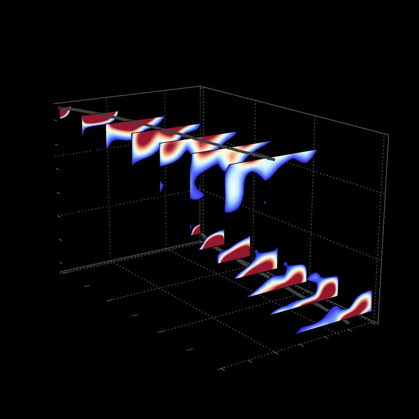
4

  a                                c                      experiment        e                              theory       g
          j                   A                                                                                               topological

                   t2          B
                        t+         y                                        y

trivial

                   t1   t-                                                                                                                     trivial

                   t2
                                                                                                                                                   experiment
                                         tim                                            tim                                                        theory
                                            e[                                             e[
                                                 mi                                          mi
                                                    n.]                                        n.]
                                   i                              x                                                 x
                                                                                                                                            time [min.]
bj                            A    d                                        f                                           h
                   t1         B
                        t+
topological

                                   y                                            y

                                                                                                                         ∆x
                   t2   t-
                   t1
                                         tim                                            tim
                                            e[                                                e[
                                                 mi                                             mi
                                   i                n.]                                           n.]               x
                                                                  x
                                                                                                                                            time [min.]
                                                                      2             P           5 x 10⁻²

Figure 2. Chiral edge motion. a, b Illustration of the stochastic network in Eq. (1) on which we superimpose the unit cell of the experimental
device (see Figs. 1 a,b). Each dot corresponds to a cell of the device and each link represents one of the transition probabilities (t1 , t2 , t+ , t− )
to move in each cardinal direction (see main text). The unit cell of this lattice is the rectangle in gray, which contains black and gray nodes
that are labelled by the sub-cell indexes A, B, respectively, introduced in Eq. (1). c-f Propagation of particles starting from the top left and
bottom right corners (the orange and green areas in a, b) for different times, for the c, e trivial and d, f topological device. We show both the c,
d experimental and e, f theoretical behaviour for (Lx , Ly ) = (13, 14). The solid lines in c-f follow the average position of the particles starting
from top left and bottom right corners. g Average position and h standard deviation in units of the cell index of a set of trajectories starting
from either top left or bottom right corners of the device, which we compare with our model (see also Supplementary Discussion 1). The active
particles of a topological device propagate faster than in a trivial device.

trivial one. Quantitatively, the time-dependent
                                    p                average dis-                       are absent for the trivial device (see Figs. 3c,d). If in addi-
                                                  2
placement hxi and spread ∆x ≡ h(x − hxi) i for particles                                tion to enforcing a vanishing probability distribution outside
starting from the top left corner, confirms this behaviour, see                         the lattice we impose that detailed balance is preserved at the
Figs. 2g and h. We observe that active particles in the topo-                           boundary, an additional edge potential partially hybridizes the
logical device are ahead of the trivial device, by about one unit                       edge modes with bulk modes, but does not remove them (see
cell after three minutes.                                                               Supplementary Discussion 1).
   The motion of active particles is understood decomposing                                 The existence of edge modes is guaranteed by a bulk Her-
Eq. (1) into the normal modes, Pk , defined by                                          mitian topological invariant. In the vertical direction the cou-
                                                                                        plings, t1 and t2 , alternate between weak and strong (see Fig.
                         Ŵ · Pk = λk Pk ,                                (2)           1b). This is the stochastic equivalent of the Su-Schrieffer-
where λk is a complex scalar which depends on wavevector                                Heeger model of the polyacetylene chain [7], which is char-
k = (kx , ky ) for periodic lattices. The real part of λk sets the                      acterized by a winding number wH in the y direction (see
lifetime of the normal mode, and its curvature ∂k2 Re(λk ) at                           Supplementary Discussion 1). wH = 1 and wH = 0 for
k = 0 sets its diffusion coefficient. The slope of the imaginary                        the topological and trivial device models, respectively. This
part ∂k Im(λk ) at k = 0 sets the velocity of the normal mode                           implies that they respectively have, or not, topological edge
(see Supplementary Discussion 1). For open boundaries along                             modes for a boundary in the y direction, indicated by black
y and periodic along x, the spectrum λk can be represented as                           arrows in Figs. 3b, d.
a function of kx . The boundary condition is such that the prob-                            The topological edge modes have a noticeable effect on the
ability distribution vanishes outside the lattice. The resulting                        edge particle dynamics of the active particles. We probe them
spectrum is shown in Figs. 3 a,b for the topological device                             by initializing Eq. (1) with a probability distribution localized
and c,d for the trivial one. The spectrum is colored according                          at the top left corner. We compare the experimental results
to the localization of the normal modes, where red and blue                             with theoretical predictions in Figs. 2e-h, using the parameters
colors denote states at the top and bottom edges, respectively.                         t1 , t2 , t+ , t− and τ set by our statistical analysis of the exper-
The normal modes localized at the edge govern the propaga-                              imental data. The theoretical curves qualitatively reproduce
tion of a particle distribution localized at an edge. Some edge                         the experimental trends without any fitting parameter, for both
modes have a chiral group velocity, shown by the slope of                               topological and trivial devices. This demonstrates that the dis-
the imaginary part of the spectrum at kx = 0 in Fig. 3b, and                            placement in the topological device is larger as a consequence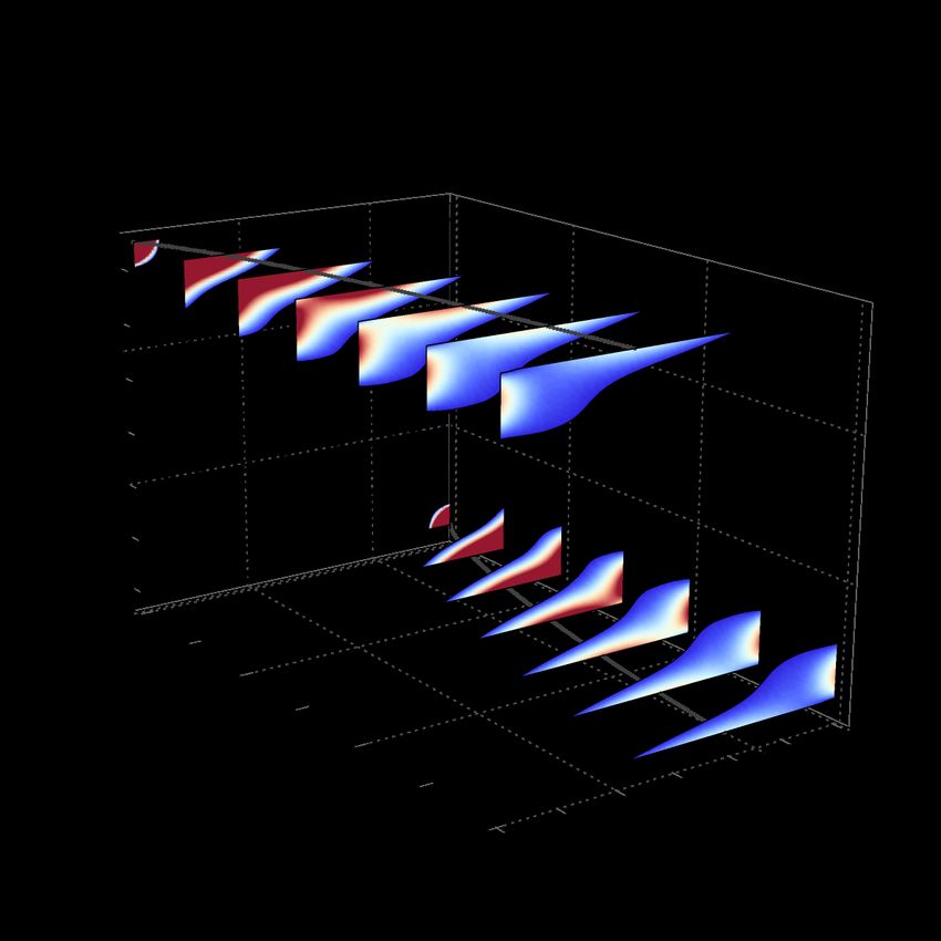
5

  a                                  c                                    plementary Discussion 1). The real part of Hs,± is finite and
               topological                         trivial
                                                                          indicates that the contribution of the topological edge modes to
                                                                          the total probability decays over a timescale τd = τ /(t1 + t2 ).

                                     Re(λ) [1/τ]
 Re(λ) [1/τ]

                                                                          τd sets how far the particles propagate due to the topological
                                                                          edge modes.
                                                                             The edge modes Hs,± have a finite 1D winding num-
                                                                          ber wnH = ±1 that implies a 1D non-Hermitian skin ef-
                                                                          fect [10, 21, 23]. Since the edge modes are spatially separated,
                                                                          active particles can accumulate at the top and bottom corners.
                                                                          We detect the accumulation of active particles experimentally
                        kx [π]                                kx [π]
                                       d                                  by post-selecting trajectories that start from a uniform config-
     b
                                                                          uration (see Fig. 1 h. and Methods). We observe an accumu-
                                                                          lation of active particles at the corners which is larger in the
                                                                          topological device (Figs. 4 a,c) and that qualitatively compares
                                     Im(λ) [1/τ]
Im(λ) [1/τ]

                                                                          with our model (Fig. 4 b,d).
                                                                             This observation can be made quantitative using the
                                                                          Shannon
                                                                             P        entropy of the particle distribution S =
                                                                          − ijσ Pijσ ln (Pijσ ). The entropy is maximal for a uniform
                                                                          distribution of particles, S < Suniform = ln(Lx Ly ), and it de-
                                                                          creases if particles localize. We average out other sources of
                         kx [π]                                kx [π]     particle localization unrelated to the non-Hermitian skin-effect
                                                                          by averaging the probability distribution over neighboring cells
                             -Ly/2                        Ly/2         (see Supplementary Discussion 2). The experimental and the-
                                                                          oretical entropies are depicted in Fig. 4 h. Both figures show
 Figure 3. Stochastic chiral edge states. Real a,c and b,d imaginary      a smaller entropy in the topological device than in the trivial
 part of the normal modes of the rate matrix Ŵ for open boundary         one. They depart from each other at the same rate, yet the
 conditions in the y direction, for the a,b topological and c,d trivial   absolute values of the experimental entropies are a factor 13
 devices. The color denotes the average hyi position of a normal
                                                                          smaller than theory. Our model thus captures the difference
 mode. Modes in green are delocalized and correspond to bulk states.
 Modes in blue and red correspond are strongly localized on the top or
                                                                          between trivial and topological devices, but underestimates
 bottom edges, respectively. The arrows in c,d highlight the presence     the accumulation that occurs in the experiment. A potential
 or absence of topological edge modes close to k = 0, where their         reason is that, in the experiment, a local increase in the number
 lifetime Re(λ) is largest.                                               of active particles leads to particle jamming, neglected in our
                                                                          model. When we decrease the density of particles to reduce
                                                                          jamming, the entropy still drops but is similar for topological
 of the topological edge modes.                                           and trivial devices. This suggests that there is a critical density
    The above observations are reproduced for smaller devices             of particles to observe corner accumulation.
 and larger densities of active particles, see Supplementary                 The corner accumulation we observe is a consequence of
 Discussion 2. We find that for larger densities, the particles           the chiral motion of topological edge modes, that accumulate
 are slower than theory predicts, an effect we attribute to particle      at the corners for long times. In the topological device the
 jamming, neglected in our model. A lower density of particles            chiral edge motion occurs because wH 6= 0, and the corner
 prevents jamming, in which case the motion compares better               accumulation occurs because wnH 6= 0 for Hs,± . The two
 with our model.                                                          devices thus have a different topological invariant
                                                                                                    ν = wH wnH ,                         (3)
        Corner accumulation from second-order non-Hermitian skin          which equals one or zero for the topological and trivial de-
                                 effect                                   vices, respectively. The topological invariant (3) highlights
                                                                          the coupled-wire nature of our system, and is reminiscent of
    The detailed balance of the unit cell implies that Ŵ has no          weak topological phases. This observation motivates different
 strong topological invariant [5] (see Supplementary Discus-              viewpoints on the higher-order topological behaviour we ob-
 sion 1). Moreover, Ŵ has inversion symmetry, implying that              serve, as we discuss in the Supplementary Discussion 1.G. In
 the first-order skin-effect vanishes.                                    the Supplementary Discussion 1.F we show that this invariant
    To derive the second-order skin effect of Ŵ we consider the          is equivalent to that in Ref. [13], and that it signals a second-
 topological edge modes, Ps,χ , at the top (χ = +) and bottom             order skin-effect as follows. First, Ŵ has inversion symmetry,
 (χ = −) described by a 1D equation τ ∂t Ps,± = Hs,± Ps,±                 and a point gap spectrum in which corner modes appear only
 (see Supplementary Discussion 1). These modes locate on                  for open-boundary conditions in both directions (Figs. 4 f, g).
 either A (for χ = +) or B (for χ = −) sub-lattice, have a                Second, the number of corner modes scales as the edge length
 ballistic propagationphxi± = ±(t+ − t− )t/τ , and diffuse by             L, rather than the system size L2 , a defining characteristic of
 an amount ∆x = (t+ + t− )t/τ after a time t (see Sup-                    the second-order the skin-effect [6].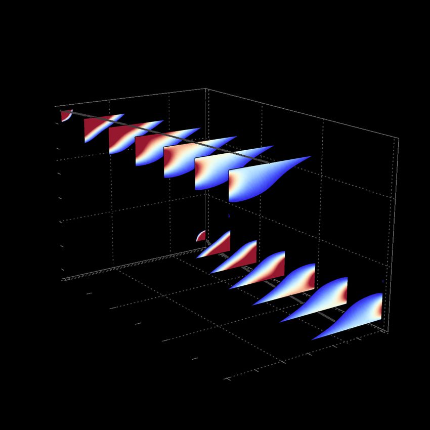
6
P (x103) P (x103)
2 6.5 3.7 6
a experiment b theory
participation ratio
g |P|
e L
Im[λ] [1/τ]
trivial
y
y
tim tim
e[ e[ 1
m m 1 x L
in. in.
c ] x d ] x Re[λ] [1/τ] h
f
S - Suniform (x 102)
topological
trivial
Im[λ] [1/τ]
y
topological
tim tim experiment
e[ e[ theory (x 13)
m m
in. in.
] x ] x
Re[λ] [1/τ] time [min.]
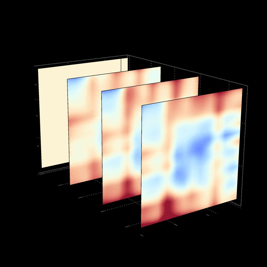
Figure 4. Second-order non-Hermitian skin effect of the active particles. a-d We compare the distribution of particles in the trivial a,c
and topological b,d devices with (Lx , Ly ) = (13, 14), observed experimentally a,b and predicted theoretically c,d. We observe that more
particles locate on the top right and bottom left corners. e,f Parametric representation of the real and imaginary parts of the spectrum of
normal modes for the P model of the trivial e and topological f devices with (Lx , Ly ) = (L, L) = (70, 70), colored with the participation ratio
of each normal mode σij |Pσij |4 , which is small for a delocalized mode. The gap in the periodic band structure is within the dashed circle
(see Supplementary Discussion 1). The number of localized modes within the point gap is proportional to the size of the device, L, and are
localized at the corners as shown in g. h Shannon entropy of the particle distribution over time. The smaller entropy in the topological device
is associated to an accumulation of particles at the corners, signaling the second-order non-Hermitian skin effect. The theoretical figures match
the experimental curves when multiplied by a factor ×13, suggesting that particle jamming, that occurs frequently for higher densities of active
particles, contributes to enhance the accumulation.
Our work establishes a strategy to design circuits that seconds, after what they are ready to be used.
spontaneously break detailed balance to guide and accu-
mulate active matter, enforced by robust out-of-equilibrium
topological phenomena. This design strategy and the 3D B. Microfabricated model substrate for topological guidance:
printing capabilities, permit to envision 3D extensions where design and fabrication
the accumulation of particles is guaranteed by non-planar
surfaces (e. g. using ramps, or different levels) [55] or by
The microscale features that define the masks are designed
implementing dynamic topographical pathways topology [56].
and microfabricated on a silicon wafer, and later transferred
by replication to a thin structure of polydimethylsiloxane
(PDMS). The microchannel design is created with a computer-
aided design (CAD) software (AutoCAD, Autodesk) and is
METHODS
made of ratchet-like structures that favor directional trajecto-
ries of the active particles [46]. Direct writing laser lithogra-
A. Particle preparation phy (DWL 66FS, Heidelberg Instruments) is used to produce
an AZr resist master (AZ 1512HS, Microchemicals GmbH)
Crystal slides of 25 × 25 mm are sequentially cleaned with of 1.5 µm thickness on the silicon wafer. A PDMS replica from
acetone and isopropanol in a sonication bath for two min- the rigid mold/master is produced to obtain the open channel
utes. The glass slides are then dried with compressed air and microfluidic device with the desired features. For reusability
treated with oxygen plasma for 10 minutes. Commercial sil- purposes, the master is silanized with trichloro (1H,1H,2H,2H-
ica microparticles (Sigma-Aldrich) of 5 µm diameter size are perfluorooctyl)sylane (Sigma-Aldrich) by vapor phase for one
deposited on the glass slides by drop-casting and left to dry at hour at room temperature, this operation reduces the adhe-
room temperature. We then sputter a 10 nm layer of Pt (Le- sion of PDMS to the substrate. To obtain a PDMS thin layer
ica EM ACE600) to integrate the catalytic layer on the silica with the inverse pattern from the rigid mold (so called PDMS
microparticles. The samples are kept in a dry and closed envi- replica), the PDMS (Sylgard 184, Dow Corning) monomer
ronment. The Janus particles are released for each experiment and cross-linker are mixed at a ratio of 10:1 and degassed for
after being briefly exposed to an Ar-plasma in order to increase one hour. Afterwards, the solution is spin-coated at 1000 rpm
their mobility. For each experiment, we dilute particles from a for 10 seconds on the top of the master and cured for 4 hours at
third of a glass slide in 1 mL of water via sonication for a few 65◦ C. The replica are carefully released, obtaining the desired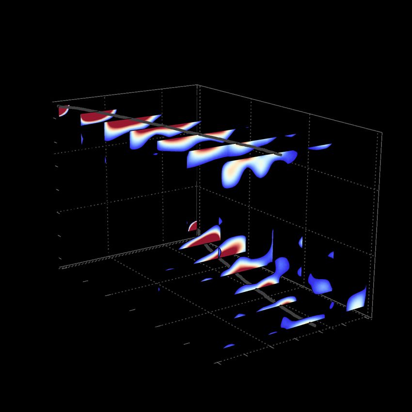
7

open microchannel designs with the sub-micrometre step-like                                    E.   Tracking
topographic features that allow the topological guidance of
active particles.                                                       In order to track a large amount of particles, we have devel-
                                                                     oped a Python script based on a neuronal network detection
                                                                     algorithm [52]. This neuronal network is taught to recognize a
                     C.   Setup fabrication
                                                                     particle from a video frame and to discard anything else. Once
                                                                     trained, we use this neuronal network to detect particles on ev-
   A circular well of 2 mm height and 1.5 cm diameter is de-         ery frame of the video. The experiments are recorded using a
signed with a CAD software and post-treated with Slic3r and          contrast microscope (Leica) with a 10x objective at 2 frames
Repetier softwares in order to generate the G-code required for      per second. A particle fits in a box of 8-9 px2 on the result-
3D printing it with a Cellink’s Inkredible+ 3D printer. Poly-        ing video. Our software relates the detected particles between
dimethylsiloxane (PDMS) SE1700 cross-linker and monomer              frames to find the trajectory of a given particle. The following
are mixed at a ratio of 1:20, and the viscous solution is added to   paragraphs detail the procedure to train the neuronal network
the cartridge used in the 3D printer. The pneumatic extrusion        and to construct trajectories from the particle we detect on
of the 3D printer allows to print the PDMS-based structures          each frame.
on clean crystal slides (60 × 24 mm) at a pressure of 200 kPa.          To train the neuronal network, we construct a dataset of
Once the well structure is printed, the slides are left overnight    images that show one or many particles. We perform this
at 65◦ C for curing, to obtain a stable structure. To ensure good    step manually by cropping a square image from a video frame.
sealing of the 3D-printed well, a mixture of 1:10 PDMS Syl-          This cropped image is centered close to a particle’s center,
gard 184 is added around the outer side of the well, followed        keeping the selected particle within, and is three times the size
by a curing period of four hours at 65◦ C.                           of a particle. We also draw a square region of the size of
   The glass slides with the 3D-printed wells are sequentially       the particle on this cropped image, like the squared, coloured,
cleaned with acetone and isopropanol, and dried with com-            boxes in Fig. 1e, that indicate the location of the particle on
pressed air. The glass substrate is activated by exposure to         the cropped image. We construct our dataset by applying this
oxygen plasma for 30 seconds. The microratchet-like patterns         procedure on many particles. We extend this dataset by also
in Sec. B are then immediately transferred to the wells to           adding cropped images that do not contain any particle. This
ensure good attachment of the patterned PDMS to the glass.           way, our dataset is composed of 8700 images with particles
The whole setup is ready and it is kept in a dry and closed          and 8700 images that do not show any particle. We input this
environment until use. Before use, the setup is cleaned with         dataset to a neuronal network based on tiny YOLOv3 [52].
a sequential wash of acetone and isopropanol, and exposed            We simplify the network by transforming the images to 8-bit
to oxygen plasma for 30 seconds. The setup design is such            grayscale and considering there are only two sizes for the boxes
that it minimizes the accumulation of gas bubbles at the center      surrounding the particles. We train the network for a day and
of the sample which permits long-time experiments, from 30           obtain a mAP-50 larger than 95%, which is sufficient for our
minutes to one hour.                                                 purpose. This generates a configuration file that we use to
                                                                     detect particles of an image. We illustrate the output of this
                                                                     detection algorithm in Fig. 1e, where an identifier is assigned
               D.   Active particles concentration                   to each detected particle.
                                                                        To build the trajectory of a particle located at position rt at
   We perform our experiment for two different concentrations        time t, we estimate that its location rt+1 at a time t + 1 is
of active particles. This allows to compare how the density of
active particles qualitatively affects our experiment. Indeed,                                         rt − rt−1
                                                                                         rt+1 = rt +             ,                 (4)
a larger density of particles enhances the Brownian motion,                                                2
due to the many collisions, but also decreases the velocity          where the second term is an estimate of the displacement of
of particles and leads to more clusters. The two densities           the particle, which is zero for the first frame since we miss the
are obtained by injecting particles in either one of the two         position r−1 . We use this position estimate to crop a square
solutions:                                                           image of the frame t + 1 centered on rt+1 and twice the size of
   1. high density of active particles. We dilute 17.5 µL of         a particle. We apply our neuronal network detection algorithm
      the solution of Janus particles prepared as detailed in        on this cropped image to detect all particles it may contain.
      the Methods describing particle preparation with 35 µL         We calculate the distance between each detected particle and
      of H2 O2 at 2% per volume and 47.5 µL of water.                each of the particles we are tracking at time t, keeping always
                                                                     the lowest distance calculated and the identification number
   2. low density of active particles. We first dilute 300 µL of     (ID) of the associated particle. We create a list with these IDs
      the solution of Janus particles prepared as detailed in the    and distances. First, we filter by selecting only those distances
      Methods describing particle preparation with 700 µL of         that have the same id as the particle we want to detect. If any,
      water. Then, we dilute 17.5 µL of this solution with           we will chose as rt+1 the closer object detected. If we cannot
      35 µL of H2 O2 at 2% per volume and 47.5 µL of water.          find the same ID, we select rt+1 as the closest object detected
This way we expect a ratio of concentrations of a third to a         to this cropped image. If finally, we have not detected any
half between high and low densities of active particles.             particle, we set rt+1 = rt . We apply this algorithm for a set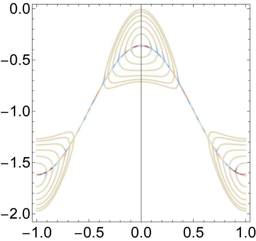
8

of particles we manually select at the initial frame, as well as              the selected trajectories, we remove all frames before
particles that may enter into the frame while recording. This                 the one where the particles first enters one of the two
tracking procedure allows to track particles even when they                   corners. This ensemble of trajectories is what we use
collide; only clogs of 5 particles or more may result in particle             for the analysis in Figs. 2 e-h.
loss. Particles may leave the sample; if this happens their
position is fixed to that frame and is removed after a period             2. Post-selected uniform. We select particles uniformly
of inactivity. Also particles can adhere electrostatically to the            scattered over the sample based on simulated annealing.
PDMS, or to each other, or be inactive. Therefore we end the                 We focus on the probability distribution Pσij (t = 0) of
trajectory if the particle is inactive for a long period of time.            all trajectories on their first frame. We scan trajecto-
We use GPU acceleration for the neuronal network detection,                  ries from the longest to the shortest and remove the first
based on the latest NVIDIA™ drivers.                                         frames of a trajectory until the newly generated distribu-
                                                                                                 0
   The filtered trajectories are given in x,y pixel coordinates,             tion of particles Pσij (t = 0) is more uniform than the
which we map to the cell coordinate of our model. This trans-                one, Pσij (t = 0), at the previous step. We consider the
formation is obtained after aligning the axes of the recorded                distribution is more uniform when
videos and decomposing the image over the lattice structure in                       v
                                                                                     uX                             2
Fig. 1 e, shown with dashed lines. We then assign each of the                                                    1
                                                                          C(P 0 ) = t          0 (t = 0) −
                                                                                     u
                                                                                              Pσij                      < C(P ). (5)
now aligned (x,y) coordinate to a cell index, using the Python                                                 Lx Ly
                                                                                        σij
library shapely.
                                                                              During this procedure, we remove trajectories that have
                                                                              less than 6 minutes of video to remove noise in the first
                F.   Post-selection of trajectories
                                                                              frames. This ensemble of trajectories is what we use for
                                                                              the analysis in Fig. 4.
   We organize the recorded trajectories in a database for each                             DATA AVAILABILITY
experimental configuration. We only keep track of the position
in the unit-cell index to eliminate any intrinsic motion of a par-
                                                                         Supplementary Information is available for this paper. The
ticle within a cell and thus to reduce noise. In the manuscript
                                                                       data that supports our finding is available on Zenodo [57].
we consider two post-selected configurations, (1) where parti-
                                                                       Additional data are available upon request.
cles start at the top left and bottom right corners (see Fig. 1g)
and, (2) where particles start from a uniform distribution (see
Fig. 1h) over the lattice. The two post-selection procedures
are as follows:
                                                                                            CODE AVAILABILITY
   1. Post-selected corner. We select particles starting from
      the corners in two steps. We first select trajectories             The code used to generate the figures is available upon
      that go through one of the two corners. Then, among              request.

 [1] M. Z. Hasan and C. L. Kane, “Colloquium: Topological insula-           (2019).
     tors,” Rev. Mod. Phys. 82, 3045–3067 (2010).                       [8] V. M. Martinez Alvarez, J. E. Barrios Vargas, and L. E. F.
 [2] Xiao-Liang Qi and Shou-Cheng Zhang, “Topological insulators            Foa Torres, “Non-hermitian robust edge states in one dimen-
     and superconductors,” Rev. Mod. Phys. 83, 1057–1110 (2011).            sion: Anomalous localization and eigenspace condensation at
 [3] Tomoki Ozawa, Hannah M. Price, Alberto Amo, Nathan Gold-               exceptional points,” Phys. Rev. B 97, 121401 (2018).
     man, Mohammad Hafezi, Ling Lu, Mikael C. Rechtsman, David          [9] Ye Xiong, “Why does bulk boundary correspondence fail in
     Schuster, Jonathan Simon, Oded Zilberberg, and Iacopo Caru-            some non-hermitian topological models,” Journal of Physics
     sotto, “Topological photonics,” Rev. Mod. Phys. 91, 015006             Communications 2, 035043 (2018).
     (2019).                                                           [10] Flore K. Kunst, Elisabet Edvardsson, Jan Carl Budich, and
 [4] CL Kane and TC Lubensky, “Topological boundary modes in                Emil J. Bergholtz, “Biorthogonal bulk-boundary correspon-
     isostatic lattices,” Nature Physics 10, 39–45 (2014).                  dence in non-hermitian systems,” Phys. Rev. Lett. 121, 026808
 [5] Suraj Shankar, Anton Souslov, Mark J. Bowick, M. Cristina              (2018).
     Marchetti, and Vincenzo Vitelli, “Topological active matter,”     [11] V. M. Martinez Alvarez, J. E. Barrios Vargas, M. Berdakin,
     arXiv e-prints , arXiv:2010.00364 (2020), arXiv:2010.00364             and L. E. F. Foa Torres, “Topological states of non-Hermitian
     [cond-mat.soft].                                                       systems,” European Physical Journal Special Topics 227 (2018).
 [6] Emil J. Bergholtz, Jan Carl Budich, and Flore K. Kunst, “Ex-      [12] Shunyu Yao and Zhong Wang, “Edge states and topological in-
     ceptional Topology of Non-Hermitian Systems,” arXiv e-prints           variants of non-hermitian systems,” Phys. Rev. Lett. 121, 086803
     , arXiv:1912.10048 (2019), arXiv:1912.10048 [cond-mat.mes-             (2018).
     hall].                                                            [13] Ching Hua Lee and Ronny Thomale, “Anatomy of skin modes
 [7] Luis E F Foa Torres, “Perspective on topological states of non-        and topology in non-hermitian systems,” Phys. Rev. B 99,
     Hermitian lattices,” Journal of Physics: Materials 3, 014002           201103 (2019).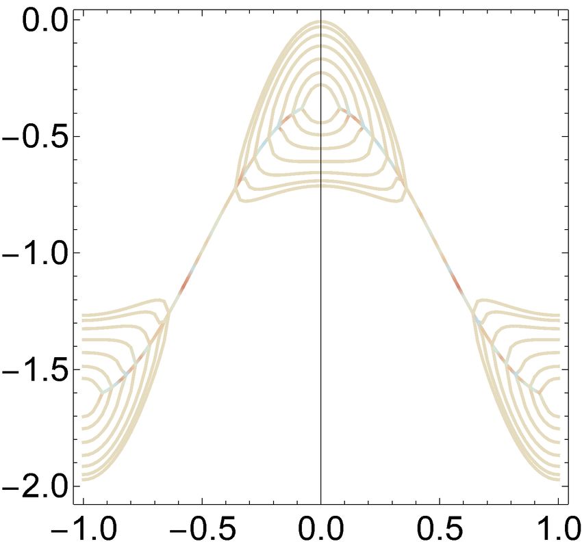
9

[14] Lei Xiao, Tianshu Deng, Kunkun Wang, Gaoyan Zhu, Zhong                    Rev. Lett. 123, 016805 (2019).
     Wang, Wei Yi, and Peng Xue, “Non-Hermitian bulk–boundary             [31] Linhu Li, Ching Hua Lee, and Jiangbin Gong, “Topological
     correspondence in quantum dynamics,” Nature Physics 16, 761–              Switch for Non-Hermitian Skin Effect in Cold-Atom Systems
     766 (2020).                                                               with Loss,” Physical Review Letters 124, 250402 (2020).
[15] Ananya Ghatak, Martin Brandenbourger, Jasper van Wezel,              [12] Yuhao Ma and Taylor L. Hughes, “The Quantum Skin
     and Corentin Coulais, “Observation of non-hermitian                       Hall Effect,” arXiv e-prints , arXiv:2008.02284 (2020),
     topology and its bulk–edge correspondence in an ac-                       arXiv:2008.02284 [cond-mat.mes-hall].
     tive mechanical metamaterial,” Proceedings of the Na-                [13] Ryo Okugawa, Ryo Takahashi, and Kazuki Yokomizo, “Second-
     tional Academy of Sciences 117, 29561–29568 (2020),                       order topological non-Hermitian skin effects,” arXiv e-prints
     https://www.pnas.org/content/117/47/29561.full.pdf.                       , arXiv:2008.03721 (2020), arXiv:2008.03721 [cond-mat.mes-
[16] Martin Brandenbourger, Xander Locsin, Edan Lerner, and                    hall].
     Corentin Coulais, “Non-reciprocal robotic metamaterials,” Na-         [6] Kohei Kawabata, Masatoshi Sato, and Ken Shiozaki, “Higher-
     ture Communications 10, 4608 (2019).                                      order non-hermitian skin effect,” Phys. Rev. B 102, 205118
[17] Yangyang Chen, Xiaopeng Li, Colin Scheibner, Vincenzo                     (2020).
     Vitelli, and Guoliang Huang, “Self-sensing metamaterials with        [14] Yongxu Fu and Shaolong Wan, “Non-Hermitian Second-
     odd micropolarity,” arXiv e-prints , arXiv:2009.07329 (2020),             Order Skin and Topological Modes,” arXiv e-prints ,
     arXiv:2009.07329 [physics.app-ph].                                        arXiv:2008.09033 (2020), arXiv:2008.09033 [cond-mat.mes-
[18] Sebastian Weidemann, Mark Kremer, Tobias Helbig, To-                      hall].
     bias Hofmann, Alexander Stegmaier, Martin Greiter, Ronny             [36] Kai Zhang, Zhesen Yang, and Chen Fang, “Universal non-
     Thomale, and Alexander Szameit, “Topological funneling of                 Hermitian skin effect in two and higher dimensions,” arXiv
     light,” Science 368, 311–314 (2020).                                      e-prints , arXiv:2102.05059 (2021), arXiv:2102.05059 [cond-
[19] T Helbig, T Hofmann, S Imhof, M Abdelghany, T Kiessling,                  mat.mes-hall].
     L W Molenkamp, C H Lee, A Szameit, M Greiter, and                    [37] Colin Scheibner, William T. M. Irvine, and Vincenzo Vitelli,
     R Thomale, “Generalized bulk–boundary correspondence in                   “Non-hermitian band topology and skin modes in active elastic
     non-Hermitian topolectrical circuits,” Nature Physics 16, 747–            media,” Phys. Rev. Lett. 125, 118001 (2020).
     750 (2020).                                                          [38] Clemens Bechinger, Roberto Di Leonardo, Hartmut Löwen,
[20] Tobias Hofmann, Tobias Helbig, Frank Schindler, Nora Salgo,               Charles Reichhardt, Giorgio Volpe, and Giovanni Volpe, “Ac-
     Marta Brzezińska, Martin Greiter, Tobias Kiessling, David                 tive Particles in Complex and Crowded Environments,” Reviews
     Wolf, Achim Vollhardt, Anton Kabaši, Ching Hua Lee, Ante                  of Modern Physics 88, 1–50 (2016).
     Bilušić, Ronny Thomale, and Titus Neupert, “Reciprocal skin          [39] Anton Souslov, Benjamin C van Zuiden, Denis Bartolo, and
     effect and its realization in a topolectrical circuit,” Phys. Rev.        Vincenzo Vitelli, “Topological sound in active-liquid metama-
     Research 2, 023265 (2020).                                                terials,” Nature Physics 13, 1091–1094 (2017).
[21] Dan S Borgnia, Alex Jura Kruchkov, and Robert-Jan Slager,            [40] Suraj Shankar, Mark J. Bowick, and M. Cristina Marchetti,
     “Non-Hermitian Boundary Modes and Topology,” Physical Re-                 “Topological sound and flocking on curved surfaces,” Phys. Rev.
     view Letters 124, 056802 (2020).                                          X 7, 031039 (2017).
[10] Nobuyuki Okuma, Kohei Kawabata, Ken Shiozaki, and                    [41] Anton Souslov, Kinjal Dasbiswas, Michel Fruchart, Suriya-
     Masatoshi Sato, “Topological origin of non-hermitian skin ef-             narayanan Vaikuntanathan, and Vincenzo Vitelli, “Topological
     fects,” Phys. Rev. Lett. 124, 086801 (2020).                              waves in fluids with odd viscosity,” Phys. Rev. Lett. 122, 128001
[23] Kai Zhang, Zhesen Yang, and Chen Fang, “Correspondence                    (2019).
     between winding numbers and skin modes in non-hermitian              [42] Kazuki Sone and Yuto Ashida, “Anomalous topological active
     systems,” Phys. Rev. Lett. 125, 126402 (2020).                            matter,” Phys. Rev. Lett. 123, 205502 (2019).
[24] Yang Yu, Minwoo Jung, and Gennady Shvets, “Zero-energy               [43] Lisa Yamauchi, Tomoya Hayata, Masahito Uwamichi, Tomoki
     corner states in a non-hermitian quadrupole insulator,” Phys.             Ozawa, and Kyogo Kawaguchi, “Chirality-driven edge flow and
     Rev. B 103, L041102 (2021).                                               non-Hermitian topology in active nematic cells,” arXiv e-prints
[25] Elisabet Edvardsson, Flore K. Kunst, and Emil J. Bergholtz,               , arXiv:2008.10852 (2020), arXiv:2008.10852 [cond-mat.soft].
     “Non-hermitian extensions of higher-order topological phases         [44] Juliane Simmchen, Jaideep Katuri, William E Uspal, Mihail N
     and their biorthogonal bulk-boundary correspondence,” Phys.               Popescu, Mykola Tasinkevych, and Samuel Sánchez, “Topo-
     Rev. B 99, 081302 (2019).                                                 graphical pathways guide chemical microswimmers,” Nature
[26] Tao Liu, Yu-Ran Zhang, Qing Ai, Zongping Gong, Kohei Kawa-                communications 7, 10598 (2016).
     bata, Masahito Ueda, and Franco Nori, “Second-order topolog-         [45] Wei Zhe Teo and Martin Pumera, “Motion Control of Micro-
     ical phases in non-hermitian systems,” Phys. Rev. Lett. 122,              /Nanomotors,” Chemistry – A European Journal 22, 14796–
     076801 (2019).                                                            14804 (2016).
[27] Motohiko Ezawa, “Non-Hermitian boundary and interface states         [46] Jaideep Katuri, David Caballero, Raphael Voituriez, Josep
     in nonreciprocal higher-order topological metals and electrical           Samitier, and Samuel Sánchez, “Directed Flow of Micromotors
     circuits,” Physical Review B 99, 121411 (2019).                           through Alignment Interactions with Micropatterned Ratchets,”
[28] Hong Wu, Bao-Qin Wang, and Jun-Hong An, “Floquet second-                  ACS Nano 12, 7282–7291 (2018).
     order topological insulators in non-hermitian systems,” Phys.        [47] Arvind Murugan and Suriyanarayanan Vaikuntanathan, “Topo-
     Rev. B 103, L041115 (2021).                                               logically protected modes in non-equilibrium stochastic sys-
[29] Jien Wu, Xueqin Huang, Jiuyang Lu, Ying Wu, Weiyin Deng,                  tems,” Nature Communications 8, 1–6 (2017).
     Feng Li, and Zhengyou Liu, “Observation of corner states in          [48] Wei Wang, Wentao Duan, Suzanne Ahmed, Ayusman Sen, and
     second-order topological electric circuits,” Phys. Rev. B 102,            Thomas E Mallouk, “From one to many: Dynamic assembly
     104109 (2020).                                                            and collective behavior of self-propelled colloidal motors,” Ac-
[11] Ching Hua Lee, Linhu Li, and Jiangbin Gong, “Hybrid higher-               counts of chemical research 48, 1938–1946 (2015).
     order skin-topological modes in nonreciprocal systems,” Phys.
10
[49] Gerhard Gompper, Roland G Winkler, Thomas Speck, Alexan- Facility, Unit 7 of ICTS “NANBIOSIS” from CIBER-BBN at
dre Solon, Cesare Nardini, Fernando Peruani, Hartmut Löwen, IBEC for their support in the masks design and fabrication.
Ramin Golestanian, U Benjamin Kaupp, Luis Alvarez, et al.,
“The 2020 motile active matter roadmap,” Journal of Physics: Author Contribution. M. G. designed the microchannel
Condensed Matter 32, 193001 (2020). designs and PDMS wells. L. P. fabricated the microchannel
[50] Ching Hua Lee, Stefan Imhof, Christian Berger, Florian Bayer,
devices, performed the experimental work and extracted the
Johannes Brehm, Laurens W Molenkamp, Tobias Kiessling,
and Ronny Thomale, “Topolectrical Circuits,” Communications corresponding data, developing also a the neural-network
Physics 1, 39 (2018). based tracking system to evaluate the trajectories of the
[2] Tobias Meng, “Coupled-wire constructions: a Luttinger liquid active Janus particles. L. P., S. T. and A. G. G. analyzed the
approach to topology,” European Physical Journal Special Top- experimental data, with input from I. P. and S. S. S. T. derived
ics 229, 527–543 (2020). the theoretical model and computed its observables. S. T. and
[52] Joseph Redmon and Ali Farhadi, “Yolov3: An incremental im- A. G. G. wrote the manuscript, with input from all authors. A.
provement,” (2018), arXiv:1804.02767 [cs.CV]. G. G. devised the initial concepts for the experimental setup
[7] W. P. Su, J. R. Schrieffer, and A. J. Heeger, “Solitons in poly- and for the theoretical modeling, and supervised the project.
acetylene,” Phys. Rev. Lett. 42, 1698–1701 (1979).
[5] Kohei Kawabata, Ken Shiozaki, Masahito Ueda, and Masatoshi Competing Interests. The authors declare that they have
Sato, “Symmetry and topology in non-hermitian physics,” Phys.
Rev. X 9, 041015 (2019).
no competing interests.
[55] Fan Yang, Fangzhi Mou, Yuzhou Jiang, Ming Luo, Leilei Xu,
Huiru Ma, and Jianguo Guan, “Flexible Guidance of Micro-
engines by Dynamic Topographical Pathways in Ferrofluids,”
ACS Nano 12, 6668–6676 (2018).
[56] Daniel Aschenbrenner, Oliver Friedrich, and Daniel F Gilbert,
“3D Printed Lab-on-a-Chip Platform for Chemical Stimulation
and Parallel Analysis of Ion Channel Function,” Micromachines
10, 548 (2019).
[57] Lucas S. Palacios, Sergueï Tchoumakov, Maria Guix, Ig-
nacio Pagonabarraga, Samuel Sánchez, and Adolfo G.
Grushin, “Dataset: Guided accumulation of active parti-
cles by topological design of a second-order skin effect,
http://dx.doi.org/%2010.5281/zenodo.4790667,” (2021).
Acknowledgements. A. G. G and S. T. are grateful to M.
Brzezinska, M. Denner, T. Neupert, Q. Marsal, S. Sayyad, and
T. Sépulcre for discussions. A. G. G and S. T acknowledge
financial support from the European Union Horizon 2020
research and innovation program under grant agreement No
829044 (SCHINES). A. G. G is also supported by the ANR
under the grant ANR-18-CE30-0001-01 (TOPODRIVE).
L. P. is grateful to J. Katuri for discussions about ratchet
design and to J. Fuentes for the PDMS wells fabrication. L.P
acknowledges financial support from MINECO for the FPI
BES-2016-077705 fellowship. M.G. thanks MINECO for the
Juan de la Cierva fellowship (IJCI2016-30451), the Beatriu
de Pinós Programme (2018-BP-00305) and the Ministry of
Business and Knowledge of the Government of Catalonia. I.P.
acknowledges support from Ministerio de Ciencia, Innovación
y Universidades (Grant No. PGC2018-098373-B-100),
DURSI (Grant No. 2017 SGR 884), and SNF (Project No.
200021- 175719). S.S. acknowledges the CERCA program
by the Generalitat de Catalunya, the Secretaria d’Universitats
i Recerca del Departament d’Empresa i Coneixement de
la Generalitat de Catalunya through the project 2017 SGR
1148 and Ministerio de Ciencia, Innovación y Universidades
(MCIU) / Agencia Estatal de Investigación (AEI) / Fondo
Europeo de Desarrollo Regional (FEDER, UE) through the
project RTI2018-098164-B-I00. S. S. acknowledge financial
support from the European Research Council (ERC) under
the European Union’s Horizon 2020 research and innovation
programme (grant agreement No 866348). All the authors ac-
knowledge MicroFabSpace and Microscopy Characterization11
Supplementary Information: Guided accumulation of active particles by topological design of a
second-order skin effect
SUPPLEMENTARY FIGURES
post-selected corner post-selected uniform
count
count
count
count
trivial
topological
count
count
count
count
Supplementary Figure 1. Distribution of characteristic times for each selection of particles for the devices with (Lx , Ly ) = (13, 14) and a
small density of active particles, for both topological and trivial devices. The timescale τ corresponds to the average time for a particle to go
from one cell to the next. The timescale T corresponds to the total length of a trajectory.
participation ratio
a b c
Im[λ] [1/τ]
Im[λ] [1/τ]
Im[λ] [1/τ]
trivial
periodic
open in x open in y open in x,y
Re[λ] [1/τ] Re[λ] [1/τ] Re[λ] [1/τ]
topological
d e edge modes f
topological
Im[λ] [1/τ]
Im[λ] [1/τ]
Im[λ] [1/τ]
periodic
open in x open in y open in x,y
Re[λ] [1/τ] Re[λ] [1/τ] Re[λ] [1/τ]
Supplementary Figure 2. Parametric representation of the real and imaginary part of the spectrum of the normal modes for the trivial a-c and
topological d-f devices, for (Lx ,Ly )=(L,L) = (70,70) lattice sites. a,d Spectrum for periodic boundary conditions in both directions (in blue)
superimposed with that for open boundary conditions in x (in red). The two spectra coincide and indicate no edge mode. b,e Spectrum for open
boundary conditions in y. The points are colored with respect to the average position hyi of the normal mode. The topological edge modes (31)
partly hybridize with bulk modes, this is seen as a gap opening forPlarger values of Re[λ]. c,f Spectrum for open boundary conditions in x and
y. The points are colored with respect to the participation ratio σij |Pσij |4 of the normal mode, a quantity which is small for delocalized
modes. As shown in the main text, the modes in the inner dashed circle are localized at the top right and bottom left corners and are related to
the second order non-Hermitian skin-effect.12
number of skin modes
L (= Lx = Ly)
Supplementary Figure 3. Number of skin modes for open boundary conditions in both x and y directions for the topological device, as a
function of system size L where (Lx , Ly ) = (L, L). This number corresponds to the number of states for open boundary conditions within the
point gap found with periodic boundary conditions (i.e. within the inner circle in Supplementary Fig. 2f). The number of skin modes increases
linearly with the perimeter, which is characteristic of a second-order non-Hermitian skin effect [6].13
small circuits large circuits
a b c d
e low density large density low density large density
topological
trivial
experiment
theory
f
∆x
g x 10-2 x 10-2 x 10-2 x 10⁻²
S - Suniform
theory x 2 theory x 2.5 theory x 4.5 theory x 13
time [min.] time [min.] time [min.] time [min.]
Supplementary Figure 4. a,b,c,d Depiction of the microfluidic devices used in our experiments. The trivial a and topological b small,
(Lx , Ly ) = (12, 6), designs, and the trivial c and topological d large, (Lx , Ly ) = (13, 14), designs. In the main text we focus on the
results obtained for the designs c and d. We consider four experimental situations with small (Lx , Ly ) = (12, 6) and large (Lx , Ly ) = (13, 14)
microfluidic devices, and with low and large density of active particles. A larger density of particles enhances the Brownian motion, but also
decreasest the velocity of particles and leads to more clusters. e,f Complementing Figs. 2g, h, we show the the time evolution of the average
position and spread for all devices, when tracking particles initially at the top left corner (see Methods, post-selection of trajectories). We
compare these quantities for the trivial and topological devices between experiments and theory. The model parameters are assigned separately
for each case, using the experimental data (see Section G), and there are no fitting parameters. g Complementing Figs. 4 e, we show the time
evolution of the entropy when tracking particles initially spread uniformly over the device (see Methods, post-selection of trajectories).14
SUPPLEMENTARY DISCUSSION 1 : STOCHASTIC MODEL OF THE DEVICE
The design of the device where the Janus particles move in is inspired by the coupled-wire construction [1–3]. In this
construction one-dimensional wires are coupled vertically to construct topological phases. Within each device we describe the
motion of active particles as a random walk described by the continuous-time Markov master equations
(
dPA,ij
τ dt = t1 (PB,i,j+1 − PA,ij ) + t2 (PB,ij − PA,ij ) + t+ PA,i−1,j − t− PA,ij + t− PA,i+1,j − t+ PA,ij ,
dPB,ij (6)
τ dt = t1 (PA,i,j−1 − PB,ij ) + t2 (PA,ij − PB,ij ) + t+ PB,i+1,j − t− PB,ij + t− PB,i−1,j − t+ PB,ij ,
where the probability distribution, Pσ,ij , is decomposed over the discrete coordinates of the network, with σ ∈ (A, B) the
2
P (see Figs. 2 a,b) and (i, j) ∈ N are the unit cell coordinates. This equation is balanced to ensure probability
sub-cell indexes
conservation, σij Pσ,ij = 1, and also, since the equation is irreducible, it has a unique stationary probability distribution with
dPst. /dt = 0 [4]. It is convenient to introduce the transition matrix Ŵ such that
dP
τ = Ŵ P, (7)
dt
where (P)σij = Pσ,ij . Eq. (6) has the form of the Schrödinger equation with a non-Hermitian Hamiltonian.
G. Experimental values
We fix the values of the parameters in Eq. (6) by counting the number of times we see a particle moving along the four types of
bulk links in the experiment. We have performed the experiment for two device sizes, (Lx , Ly ) = (12, 6) and (Lx , Ly ) = (13, 14)
(see Figs. 4 a-d) and, for a low and a high density of active particles (see Methods, Experimental Setup).
For each situation we obtain the following transition probabilities
1. For our largest device, with (Lx , Ly ) = (13, 14), and a low density of active particles:
• (t1 , t2 , t+ , t− ) = (0.154, 0.212, 0.512, 0.122) for the trivial device,
• (t1 , t2 , t+ , t− ) = (0.214, 0.128, 0.545, 0.112) for the topological device.
These are the values we use to compare our experiment with the model in Figs. 3 c,d.
2. For our largest device, with (Lx , Ly ) = (13, 14), and a high density of active particles:
• (t1 , t2 , t+ , t− ) = (0.126, 0.206, 0.461, 0.207) for the trivial device,
• (t1 , t2 , t+ , t− ) = (0.203, 0.119, 0.466, 0.212) for the topological device.
These are the values we use to compare our experiment with the model in Figs. 4 e.
3. For our smallest device, with (Lx , Ly ) = (12, 6), and a low density of active particles:
• (t1 , t2 , t+ , t− ) = (0.150, 0.199, 0.519, 0.132) for the trivial device,
• (t1 , t2 , t+ , t− ) = (0.179, 0.123, 0.579, 0.119) for the topological device.
4. For our smallest device, with (Lx , Ly ) = (12, 6), and a high density of active particles:
• (t1 , t2 , t+ , t− ) = (0.143, 0.191, 0.514, 0.152) for the trivial device,
• (t1 , t2 , t+ , t− ) = (0.215, 0.125, 0.541, 0.120) for the topological device.
We observe an asymmetry between vertical and horizontal motions since t1 + t2 = 0.33 < 0.67 = t+ + t− ; the motion along
the horizontal axis is easier because the ratchets are aligned while vertical micro-channels are not. This asymmetry in the design
is a consequence of the spatial constraints during device fabrication and it also helps to distinguish better topological and trivial
devices in the experiment. Indeed, the contribution of topological edge modes to the displacement of particles is largest for an
asymmetric network with t1 + t2 < t+ + t− , because it increases the decay time τd = τ /(t1 + t2 ) of the edge modes. This
condition is satisfied in the present experiment because the ratchets favour the horizontal motion of the Janus particles. Also,
one can expect to observe a ballistic regime after a time
τb = (t+ + t− )τ /(t+ − t− )2 , (8)You can also read