Image Denoising Using a Compressive Sensing Approach Based on Regularization Constraints

Preprints (www.preprints.org) | NOT PEER-REVIEWED | Posted: 27 January 2022 doi:10.20944/preprints202201.0411.v1

 Article

 Image Denoising Using a Compressive Sensing Approach
 Based on Regularization Constraints
 Assia El Mahdaoui1, Abdeldjalil Ouahabi2,* and Mohamed Said Moulay 1

 1 Dept. of Analysis, AMNEDP Laboratory, University of Sciences and Technology Houari Boumediene,
 16111 Algiers, Algeria; aelmahdaoui@usthb.dz; mmoulay@usthb.dz
 2 UMR 1253, iBrain, INSERM, University of Tours, 37000 Tours, France

 * Correspondence: ouahabi@univ-tours.fr

 Abstract: In remote sensing applications, one of the key points is the acquisition, real-time pre-
 processing and storage of information. Due to the large amount of information present in the form
 of images or videos, compression of this data is necessary. Compressed sensing (CS) is an efficient
 technique to meet this challenge. It consists in acquiring a signal, assuming that it can have a sparse
 representation, using a minimal number of non-adaptive linear measurements. After this CS
 process, a reconstruction of the original signal must be performed at the receiver. Reconstruction
 techniques are often unable to preserve the texture of the image and tend to smooth out its details.
 To overcome this problem, we propose in this work, a CS reconstruction method that combines the
 total variation regularization and the non-local self-similarity constraint. The optimization of this
 method is performed by the augmented Lagrangian which avoids the difficult problem of non-
 linearity and non-differentiability of the regularization terms. The proposed algorithm, called
 denoising compressed sensing by regularizations terms (DCSR), will not only perform image
 reconstruction but also denoising. To evaluate the performance of the proposed algorithm, we
 compare its performance with state-of-the-art methods, such as Nesterov's algorithm, group-based
 sparse representation and wavelet-based methods, in terms of denoising, and preservation of edges,
 texture and image details, as well as from the point of view of computational complexity. Our
 approach allows to gain up to 25% in terms of denoising efficiency, and visual quality using two
 metrics: PSNR and SSIM.

 Keywords: compressive sensing; image reconstruction; regularization; total variation; augmented
 Lagrangian; non-local self-similarity; wavelet denoising

 1. Introduction
 Compressed sensing (CS) has already attracted great interest in various fields.
 Examples include medical imaging [1,2], communication systems [3–6], remote sensing [7],
 reconstruction algorithm design [8], image storage in databases [9], etc. Compressed
 sensing provides an alternative approach to Shannon vision to reduce the number of
 samples, and/or reduce transmission/storage costs. There are other approaches that also
 address this issue, such as random sampling [10]. Compressed sensing recovery is a linear
 optimization problem. The most common CS retrieval algorithms explore the prior
 knowledge that a natural image is sparse in certain domains, such as in the wavelet
 domain, where simple and efficient noise reduction is possible [11–14], or in the discrete
 gradient domain that we will develop in this work.
 Image recovery in these application domains can be formulated as a linear inverse
 problem, which can be modeled as follows:

 f=Au+ε (1)

 ∈ ℝ is the observed noisy image, ∈ ℝ is the unknown clean image, and ε is an
 additive noise and ∈ ℝ × is a linear operator. Given , image reconstruction extract ̂

 © 2022 by the author(s). Distributed under a Creative Commons CC BY license.

Preprints (www.preprints.org) | NOT PEER-REVIEWED | Posted: 27 January 2022 doi:10.20944/preprints202201.0411.v1

 from making classical least-squares approximation alone not suitable. To stabilize
 recovery, regularization techniques frequently used, giving a general reconstruction model
 of the form:
 1
 arg min ‖ − ‖22 + ( ), (2)
 2

 where, > 0 is a regularization parameter and ‖ ‖2 denotes the 2 norm. The fidelity
 term, ‖ − ‖22 , forces the reconstructed image to be close to the original image. The
 regularization term, ( ), actually perform the noise reduction.
 Many optimization approaches for regularization based image inverse problems have
 been developed. Particularly, the total variation (TV) based approach has been one of the
 most popular and successful approaches; Chambolle [15] introduced the dual approach to
 the unconstrained real valued case. Later, Beck and Teboulle [16] present a fast
 computational method based on gradient optimization approach for solving the TV-
 regularized problem. Recently, several methods based on total variation have been
 proposed for hyperspectral image [17,18] denoising an essential preprocessing step to
 improve image quality.
 However, since the total variation model favors the piecewise constant image
 structures, the total variation models tend to over smooth the image details, it tends to
 smooth out the fine details of an image. To overcome these intrinsic draw backs of the total
 variation model, we introduce a non-local self-similarity constraint, as a complementary
 regularization into the model. The non-local self-similarity can restore high quality image.
 To make our algorithm robust, an augmented Lagrangian method is proposed to solve
 efficiently the above inverse problem.
 The remainder of this paper is organized as follows. In section 2, the basics of the
 methods used to image restoration are presented. The tools of denoising image considered
 in the proposed framework are described in section 3. Section 4 presents our proposed
 algorithm, called DCSR. The experimental results from the processing of Lena, Barbara
 and Cameraman images, available in the public and royalty-free, database
 https://ccia.ugr.es/cvg/dbimagenes/index.php, and the comparison with competing
 methods are discussed in Section 5. Finally, conclusions are given in Section 6.

 2. Related Works
 2.1. Compressive sensing
 The aim of compressive sensing [19,20] is to acquire an unknown signal, assuming to
 have a sparse representation while using the minimal number of linear non adaptive
 measurements. After wards, recover it by means of efficient optimization procedures. The
 three points of compressive sensing theory are the sparsity of the received signals,
 incoherent measurement matrix and robust algorithm of reconstruction.
 Let ∈ ℝ be a signal having a sparse representation and its sparsity is , ( ≪ ),
 so that can be expressed as:

 = (3)

 where, = ( 1 , 2 , … , ) is the basis matrix, ∈ ℝ ×1 the column vector of weighting
 coefficients with

 = ⟨ , ⟩ = (4)

 using ∈ ℝ × as a sensing matrix of dimension < ≪ . The obtained signal is:

 = = (5)

Preprints (www.preprints.org) | NOT PEER-REVIEWED | Posted: 27 January 2022 doi:10.20944/preprints202201.0411.v1

 with = −1 . is an × matrix that verifies the restricted isometry condition of
 order :

 ‖ ‖2
 2
 1 − ≤ ‖ ‖2
 ≤ 1 + , 0 < < 1 (6)
 2

 The reconstruction of from can be obtained via the 1 norm minimization as:

 ̂ = min ‖ ‖1 subject to = (7)

 More often, when is contaminated by noise, the equality constraint comes:

 ̂ = min‖ ‖1 subject to ‖ − ‖22 ≤ (8)

 where > 0 represents a predetermined noise level. For an appropriate scalar weight
 , we can obtain the following variant of (8):

 1 (9)
 min ‖ − ‖22 + ‖ ‖1
 2

 Problems (8) and (9) are equivalent in the sense that solving one will determine the
 parameter in the other such that both give the same solution. If is sufficiently sparse and
 the measurement matrix is incoherent with orthogonal basis , then can be
 reconstructed by solving the 1 norm minimization problem.
 There are several iterative reconstruction algorithms to solve the problem, such as
 orthogonal matching pursuit (OMP) [21] and approximate message passing (AMP) [22],
 an extension of the AMP; denoising based AMP (D-AMP) [23] employs denoising
 algorithms for CS recovery and can get a high performance for nature images.

 2.2. Augmented Lagrangian
 Augmented Lagrangian method [24] is a new technique that appears with the core
 idea, which is a combination between the standard Lagrangian function and quadratic
 penalty function, also known as the method of multipliers.
 Considering the following constrained optimization problem:

 min ( ) subject to = (10)
 
 where ∈ ℝ , ∈ ℝ and is a matrix of dimension × , i.e., there are linear
 equality constraints.

 The augmented Lagrangian function for this problem is given by:

 ( , , ) = ( ) − λT ( − ) + ‖ − ‖22 (11)
 2

 such as, ∈ ℝ is a vector of the Lagrange multiplier and > 0 is the augmented
 Lagrangian penalty parameter for the quadratic infeasibility term [25]. As described in
 Algorithm 1, the so-called augmented Lagrangian method consists in finding the global
 optimal point of the optimization problem, which has two vectors, the Lagrangian
 multiplier λ and the signal , that need to be solved. Through the alternate iteration
 method to keep one vector fixed and to update the other, the solution can be obtained
 successfully until the stopping criterion is satisfied.

Preprints (www.preprints.org) | NOT PEER-REVIEWED | Posted: 27 January 2022 doi:10.20944/preprints202201.0411.v1

 Algorithm 1: Augmented Lagrangian method
 Initialization: = 0, > 0, 0 , 0
 Iterations : for = + 1 until the stopping criterion is
 satisfied, repeat steps 1-2
 1. Keep fixed and update :
 
 +1 = min ( ) − ( − ) + ‖ − ‖22
 2
 2. Keep fixed and update :
 +1 = + ( +1 − )
 Output : the optimal solution.

 3. Technical framework for image denoising
 It is well known that existing several methods for image denoising, including total
 variation image regularization [26], wavelet thresholding [27], non-local means [28], basis
 pursuit denoising [29], block-matching and 3D filtering [30], among others. These
 methods can perform image smoothing/denoising as well as preserve edges to a certain
 extent. If we can obtain more precise measurements of the original images than the
 corresponding noisy images, then we can reconstruct the image well by CS theory. In
 particular, we can them into two classes, as special cases of the proposed framework.

 3.1. Regularization functions
 The total variation has been introduced in first by Rudin, Osher and Fatemi [31], as a
 regularizing criterion for solving inverse problems. Total variation model is a
 regularization terms demonstrate high effectiveness in preserving edges and recovery
 smooth regions. The use of total variation regularization in the area of compressive
 sensing makes the reconstructed images sharper by preserving the edges or boundaries
 more accurately. Then, the total variation (TV) model can be written as:
 ( ) = ‖ ‖ (12)
 where ∈ ℝ represents an image, = [ ℎ , ] and ℎ , denote the horizontal and
 vertical gradient picture, respectively. The norm could either be the 2 norm
 corresponding to the isotropic TV, or the 1 norm corresponding to the anisotropic TV. By
 1
 definition, norm is ‖ ‖ = ( ∑ 
 =1| | ) . In this paper, we consider equal to 1.

 A non-local self-similarity (NLS) is another significant property of natural images, it
 was proposed in the first time in the work for image denoising [32]. It depicts the
 repetitiveness of the textures [33,34] or structures embodied by natural images, which is
 maintaining properties of initial image (the sharpness and edges) and obtaining in this
 steps. First, it divides image size into many overlapped blocks of size √ × √ ,
 at location , = 1, 2, . . , . Second, search ( − 1) similar blocks and denoted a set
 including best block to in the training window with ( × ) size. Third, for each 
 transform the blocks belonging to into 3D array by the superposition denoted by .

 ( ) = ‖ ‖1 = ∑ ǁ 3 ( )ǁ1 (13)
 1

 such that 3 is the operator of an orthogonal 3D transform, and 3 ( ) the
 transform coefficients for . be the column vector of all the transform coefficients
 of image with size = √ × √ × built from all the 3 ( ) arranged in the
 lexicographic order.

Preprints (www.preprints.org) | NOT PEER-REVIEWED | Posted: 27 January 2022 doi:10.20944/preprints202201.0411.v1

 3.2. Wavelet denoising
 Wavelet shrinkage denoising attempts to remove whatever noise present and retain
 whatever signal is present regardless of the frequency content of the signal. In the wavelet
 domain, the energy of a natural signal is concentrated in a small number of coefficients;
 noise is, however, spread over the entire domain. The basic wavelet shrinkage denoising
 algorithm consist of three steps:
 • Discrete wavelet transform (DWT) [35];
 • Denoising [36];
 • Inverse DWT.
 The following is the measurement model:

 = + (14)
 where, is the original image of size × corrupted by an additive noise . The goal
 is to estimate the denoised image ̂ from noisy observation . The elimination of this
 additive noise can be under the assumption that the appropriate choice of decomposition
 basis allows discrimination of the useful signal (image) from noise. This hypothesis
 justifies, in part, the traditional use of denoising by thresholding. There are two
 thresholding methods frequently used. The soft-thresholding function (also called the
 shrinkage function):

 ( ) − if ( ) > 
 ̂ ( ) = { ( ) + if
 
 ( ) < − (15)
 
 0 otherwise

 The other popular alternative is the hard-thresholding function:

 ( ) | ( )| > (16)
 ̂ ( ) = {
 0 ℎ 
 
 such that, ( ) is the wavelet coefficients of the measured signal at level , the
 estimation of the wavelet coefficients of the useful signal, denoted ̂ ( ) with the
 threashold = √2 , where is the number of pixels for the test image and 
 represents the noise standard deviation.

 4. Our efficient image denoising scheme
 In what follows, we substitute the aforementioned results (12) and (13) into (9), we
 obtain the following problem :

 1
 arg min ‖ − ‖22 + ( ) + ( ) (17)
 2
 Lets us recall that ( ) = ‖ ‖1 and ( ) = ‖ ‖1 = ∑ 
 1 ǁ 
 3 
 ( )ǁ1

 The problem can be converted into an equality-constrainted problem by
 introducing and ,

 1
 min ‖ − ‖22 + ‖ ‖1 + ‖ ‖1 subject to = , = (18)
 , , 2

 where and are control parameters. Augmented Lagrangian function of (18) is as follow:

 1 
 ℒ ( , , ) = ‖ − ‖22 + ‖ ‖1 + ‖ ‖1 − ( − ) − ( − ) + ‖ − ‖22 + ‖ − ‖22 (19)
 2 2 2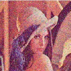

Preprints (www.preprints.org) | NOT PEER-REVIEWED | Posted: 27 January 2022 doi:10.20944/preprints202201.0411.v1

 where and are the penalty parameters corresponding to ‖ − ‖22 and ‖ − ‖22
 respectively.
 To solve (18), we use the augmented Lagrangian method iteratively, as follow:

 ( +1 , +1 , +1 ) = arg min ℒ ( , , )
 , , 
 { +1 = − ( +1 − +1 ) (20)
 +1 = − ( +1 − +1 )

 Here, the subscript denotes the index of the iteration and , are the Lagrangian
 multipliers associated with the constraints = , = , respectively.
 Due to the non differentiability of problem (19), we used the alternative direction
 method to solve efficiently a problem, which alternatively minimizes one variable while
 fixing the other variables, to split (19) into the following three sub-problems. For
 simplicity, the subscript is omitted without confusion.

 • Update 
 Given and , the optimization problem associated with as follow:
 
 arg min ‖ ‖1 − ( − ) + ‖ − ‖22 (21)
 2

 according to [37], the solution of w sub-problem is written as:

 ̃ = max {| − | − , 0} sgn ( − ) (22)
 
 where max {∙} represents the larger number between two elements, and sgn(∙) is a is a
 piecewise function defined as follows:
 −1 if < 0
 sgn( ) = { 0 if = 0
 1 if > 0

 • Update 
 Given and , the sub-problem associated with is equivalent to

 1 
 arg min ‖ − ‖22 − ( − )− ( − ) + ‖ − ‖22 + ‖ − ‖22 (23)
 2 2 2

 which simplifies to the linear system

 1 1 
 ( + ( + ) ) = + ( − ) + ( − ) (24)
 
 We observe that is a positive semi definite tridiagonal matrix. Since and are both
 positive scalars, the matrix on the left-hand-side of the above system is positive definite
 tridiagonal.

 • Update 
 Given and , the sub-problem becomes

 arg min ‖ ‖1 + ‖ − ‖22 − ( − ) (25)
 2
 the problem (25) can be reformulated below: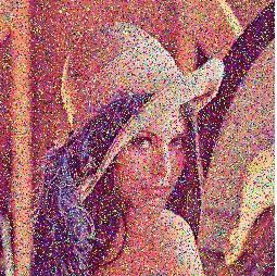

Preprints (www.preprints.org) | NOT PEER-REVIEWED | Posted: 27 January 2022 doi:10.20944/preprints202201.0411.v1

 1 
 arg min ‖ − ‖22 + ‖ ‖1 (26)
 2 

 Considering = − with = , as a noisy observation of , the error (or noise) = −
 
 follows a probability law, not necessarily Gaussian, with zero mean and variance 2 .
 According to the central limit theorem or law of large numbers, the following equation
 holds:
 1 1
 ‖ − ‖22 = ‖ − ‖22 (27)
 
 with , , ∈ ℝ and , ∈ ℝ for = 1, … , 
 equivalent to

 ‖ − ‖22 = ‖ − ‖22 (28)
 
 incorporating (28) into (26) leads to
 1 
 arg min ‖ − ‖22 + ‖ ‖ (29)
 2 1
 since the unknown variable is component-wise separable in (29), such that

 ̂ = soft( , √2 ),
 = , = √ × √ × (30)
 
 ̂ = sgn( ) max{| | − √2 , 0}
 (31)

 Thus, the closest solution from sub-problem (25) is follow:

 ̂ )
 ̃ = Ω( 
 (32)

 where Ω is the reconstruction operator.
 Based on the discussions above, we get the algorithm for solving (17) shown below:

 Algorithm 2: The proposed algorithm (DCSR)
 Input: The observed measurement , the measurement matrix 
 Initialization: 0 = 0 = 0, 0 = , 0 = 0 = 0
 while Outer stopping criteria unsatisfied do
 while Inner stopping criteria unsatisfied do
 solve sub-problem by computing equation (22)
 solve sub-problem by computing equation (24)
 solve sub-problem by computing equation (32)
 end while
 Update multipliers by equation (20)
 end while
 Output : The final image is restored.

 The algorithm detailed above is used to recover corrupted images by white Gaussian
 noise and salt pepper noise.
 Comparative performance of competing methods to recovery noisy images is
 discussed in the next section.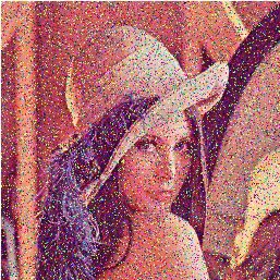

Preprints (www.preprints.org) | NOT PEER-REVIEWED | Posted: 27 January 2022 doi:10.20944/preprints202201.0411.v1

 5. Experimental results and discussion
 In this section, we describe the experiments undertaken with both simulated and real
 data sets to verify the efficiency and practicability of the proposed method. To evaluate
 the performance of the proposed algorithm, DCSR, we compare it with three other
 popular CS recovery algorithms: The first algorithm, wavelet thresholding, denoising
 natural images by assuming they are sparse in the wavelet domain. It transforms signals
 into a wavelet basis, thresholds the coefficients, and then inverses the transform. The
 second algorithm, NESTA is based on Nesterov’s smoothing technique, extended to TV
 minimization by modifying the smooth approximation of the objective function. The third
 algorithm, group-based sparse representation (GSR) enforces image sparsity and self-
 similarity simultaneously under a unified framework in an adaptive group domain.
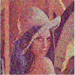
 We used three images, Barbara and Cameraman gray-scale images with size of
 256 × 256 and color Lena image 512 × 512 in our experiments, see Figure 1.

 (a) (b) (c)
 Figure 1. Test images used in the experiments. (a) Barbara, (b) Cameraman, (c) Lena.

 In the simulations, two types of noise were used: the additive white Gaussian noise
 (AWGN) measured by its standard deviation and its mean and the salt and pepper
 noise.
 The salt and pepper noise on image has the following form:
 with probability 1
 ( ) = { (33)
 with probability 2

 where = ( 1 , 2 , … , ) ∈ ℝ pixels and is the pixel intensity of salt pixels and 
 is the pixel intensity of pepper pixels. The sum = 1 + 2 is the level of the salt and
 pepper noise.

 5.1. Visual Quality Comparison
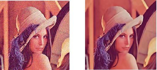
 First, we evaluate the performance of our DCSR algorithm by performing
 experiments on Barbara image corrupted by white Gaussian noise with standard
 deviation ranging from 20 to 80. Figure 2 shows the recovery image results with
 different values of noises .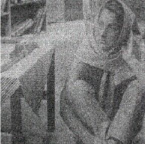

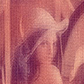
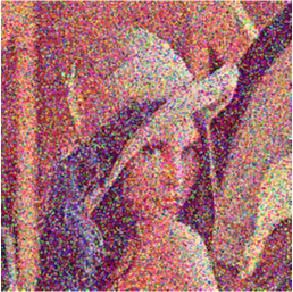
Preprints (www.preprints.org) | NOT PEER-REVIEWED | Posted: 27 January 2022 doi:10.20944/preprints202201.0411.v1

 (a) (b) (c) (d)

 Figure 2. Visual comparison of the reconstruction quality of the proposed DCSR algorithm for
 different noise levels. (a) = 20, (b) = 50, (c) = 60, (d) = 80.

 From Figure 2, it can be seen that the details of Barbara image are preserved very well
 after denoising with noise from 20 to 80.
 The pleasant visual quality is important for a viewer. In order to verify the
 superiority of the proposed method, we compare it with GSR algorithm, wavelet
 denoising and NESTA algorithm. We obtain a recovered image from each solver.
 Comparison experiments are shown in Figures 3, 4 and 5.

 (a) (b) (c) (d)

 Figure 3. Visual comparison of the reconstruction quality of GSR algorithm for different noise levels.
 (a) = 20, (b) = 50, (c) = 60, (d) = 80.

 (a) (b) (c) (d)

 Figure 4. Visual comparison of the reconstruction quality of the wavelet denoising algorithm for
 different noise levels. (a) = 20, (b) = 50, (c) = 60, (d) = 80.

 (a) (b) (c) (d)
 Figure 5. Visual comparison of the reconstruction quality of NESTA algorithm for different noise
 levels. (a) = 20, (b) = 50, (c) = 60, (d) = 80.

Preprints (www.preprints.org) | NOT PEER-REVIEWED | Posted: 27 January 2022 doi:10.20944/preprints202201.0411.v1

 This image Barbara is relatively complex with rich texture and geometry structure.
 The images reconstructed by NESTA algorithm are visually unpleasant and lose some
 important details, for wavelet denoising if the standard deviation is set too large
 (greater than 50) the image noise can not be suppressed. Also, one can see that GSR is
 effective in suppressing the noises. By comparing, the proposed method provides the
 most visually pleasant results in both edges and textures.
 Secondly, we handle the proposed approach to process the impulsive noise salt and
 pepper in various noise levels varying from 20% to 70% and compared its denoising
 performance with several denoising algorithms: GSR algorithm, NESTA algorithm and
 wavelet denoising. Figure 6 provides visual results for different algorithm and several
 noise levels, it can be found that the image Cameraman has been reconstructed very well
 by our algorithm, DCSR, even with high noise level greater than 50%. We can conclude
 that DCSR method presents the best quality image compared to other methods.

 Noise level 20%

 Noise level 50%

 Noise level 60%

 Noise level 70%

 Figure 6. Visual comparison of the reconstruction quality for different noise levels in the case of salt
 and pepper (see column 1 located on the left side). The algorithms used are, DCSR, GSR, wavelet
 denoising and NESTA: The denoised images are arranged in columns 2, 3, 4 and 5 respectively.

Preprints (www.preprints.org) | NOT PEER-REVIEWED | Posted: 27 January 2022 doi:10.20944/preprints202201.0411.v1

 5.2. Image Quality Metrics
 The image processing community has long been using PSNR and MSE as fidelity
 metrics. The formulas are simple to understand and implement; they are easy and fast to
 compute and minimizing MSE is also very well understood from a mathematical point of
 view.
 PSNR (peak signal-to-noise ratio, unit: dB) [38] is the ratio between the maximum
 possible power of a signal and the power of noise. The higher PSNR value means the better
 visual quality. PSNR is defined as follows:
 2
 (2 −1)
 PSNR = 10 log10 (34)
 MSE

 1 2
 MSE = ∑ ∑( ( , ) − ̂( , )) (35)
 
 =1 =1

 MSE represents the mean square error between two images, is the initial image and ̂ is
 the reconstructed image of size × , and represent the image row and column pixel
 position respectively, is the number of bits of each sample value.
 As an alternative to data metrics described above, better visual quality measures
 have been designed taking into account the effects of distortions on perceived quality.
 Note that, structural similarity (SSIM) textures [39] is a proven to be a better error metric
 for comparing the image quality and it is in the range [0, 1] with value closer to one
 indicating better structure preservation.

 SSIM = ( , ̂) × ( , ̂) × ( , ̂) (36)

 such that, ( , ) is the luminance comparison defined as a function of the mean
 intensities and of signals and :
 2 + 1
 ( , ) = (37)
 2 + 2 + 1
 The contrast comparison ( , ) is a function of standard deviations and , and
 takes the following form:

 2 + 2
 ( , ) = (38)
 2 + 2 + 2

 The structure comparison ( , ) is defined as follows:

 + 3
 ( , ) = (39)
 + 3

 where, and represent the mean value of images and ̂ respectively. 2 and 2
 represent the variance of images and ̂ respectively. is the covariance of images 
 and ̂. 1 , 2 and 3 are constants.
 Specifically, it is possible to choose = 2 2 , = 1 and is a constant,
 such as ≪ 1 and is the dynamic range of the pixel values ( = 255 corresponds to a
 grey-scale digital image when the number of bits/pixel is 8).

Preprints (www.preprints.org) | NOT PEER-REVIEWED | Posted: 27 January 2022 doi:10.20944/preprints202201.0411.v1

 5.3. Quantitative assessment
 In this sub-section, we evaluate the quality of image reconstruction. We compare
 these methods furthermore quantitatively; the peak signal to noise ratio (PSNR) and
 structural similarity (SSIM) indices are calculated for the images with different algorithms.
 Remember that, at first gray image Barbara was contaminated by Gaussian white
 noise with different values of standard deviation σ and denoising with different
 algorithms. The results of the PSNR values by various algorithms are shown in Figures 7-
 10. Let us recall that, the higher PSNR indicates superior image quality and a good
 performance of algorithm. The values of PSNR illustrate that, obviously, DCSR yields a
 higher PSNR than the other three methods.

 PSNR: 38.75 dB PSNR: 35.16 dB PSNR: 34.67 dB PSNR: 33.59 dB

 Figure 7. PSNR for different noise levels using the proposed DCSR. From left to right = 20, 50,
 60 and 80 respectively.

 PSNR: 34.07 dB PSNR: 29.10 dB PSNR: 27.39 dB PSNR: 24.49 dB

 Figure 8. PSNR for different noise levels using GSR algorithm. From left to right = 20, 50, 60 and
 80 respectively.

 PSNR: 27.03 dB PSNR: 20.18 dB PSNR: 19.02 dB PSNR: 17.45 dB

 Figure 9. PSNR for different noise levels using wavelet denoising. From left to right = 20, 50, 60
 and 80 respectively.

Preprints (www.preprints.org) | NOT PEER-REVIEWED | Posted: 27 January 2022 doi:10.20944/preprints202201.0411.v1

 PSNR: 24.19 dB PSNR: 19.15 dB PSNR: 18.08 dB PSNR: 15.46 dB

 Figure 10. PSNR for different noise levels using NESTA algorithm. From left to right = 20, 50,
 60 and 80 respectively.

 Figure 11 presents the performance analysis of four denoising methods for grayscale
 image corrupted by additive white Gaussian noise. We can clearly see that DCSR our
 algorithm exhibits the best performance with high PSNR (low noise level) and also with
 low PSNR (high noise level).

 Figure 11. Grayscale image corrupted by additive white Gaussian noise (AWGN): Performance
 analysis of four denoising methods.

 To quantitatively evaluate the effectiveness of our reconstruction-de-noising method,
 the test image used is corrupted by salt and pepper noise with different noise levels.. Table
 1 shows the quantitative assessment results PSNR and SSIM of our algorithm, DCSR, for
 several values of the noise levels, as well as results obtained using GSR, wavelet and
 NESTA.

Preprints (www.preprints.org) | NOT PEER-REVIEWED | Posted: 27 January 2022 doi:10.20944/preprints202201.0411.v1

 Table 1. Quality metrics results on different algorithms for different values of noise levels.

 Method Noise level PSNR SSIM
 20% 33.97 0.99
 Ours (DCSR) 50% 30.08 0.95
 60% 27.03 0.93
 70% 25.24 0.92
 20% 26.70 0.80
 GSR algorithm 50% 24.66 0.78
 60% 23.61 0.74
 70% 22.40 0.69
 20% 31.68 0.89
 Wavelet denoising 50% 28.61 0.86
 60% 26.69 0.79
 70% 24.84 0.74
 20% 18.88 0.39
 NESTA algorithm 50% 16.71 0.38
 60% 16.33 0.37
 70% 16.03 0.36
 The best results are highlighted in bold type font. Table 1 indicates that, the PSNR and
 SSIM values obtained by NESTA are lower, indicating that there are a limitation on the
 restoration images although being a successful image recover method. GSR and wavelet
 obtain intermediate PSNR values and SSIM values. Table 1 validates that our method has
 superiority in image reconstruction compared with the three methods.
 This performance is confirmed by Figure 12 which illustrates the PSNR output
 variations with respect to the input PSNR.

 Figure 12. Grayscale image corrupted by salt and pepper noise: Performance analysis of four
 denoising methods.

 The next challenge is to apply this DCSR algorithm to color, or multidimensional,
 images. This is esential since most digital images used in the modern world are not
 grayscale, but usually operate in either the RGB or YCbCr color spaces. Both these colors
 paces are 3-dimensional.
 We evaluate the proposed DCSR algorithm on color image Lena. Lena is a good test
 image because it has a nice mixture of detail, flat regions, shading area and texture. We
 mainly compare our proposed method to wavelet denoising and GSR algorithm.

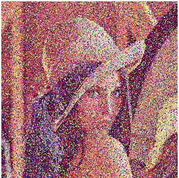
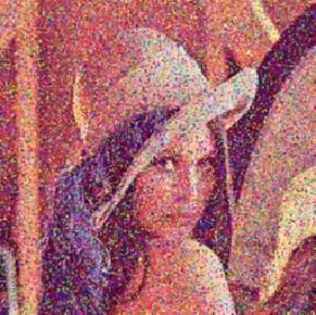
Preprints (www.preprints.org) | NOT PEER-REVIEWED | Posted: 27 January 2022 doi:10.20944/preprints202201.0411.v1

 As mentioned previously, two types of noise are used in these experiments: AWGN with
 a standard deviation and several salt and pepper noise levels.
 At the beginning, additive white Gaussian noise with different values of standard
 deviation = 20, 50, 60 and 80 are added to this testing image to generate the noisy
 observations.
 Denoising results of this image with different algorithm are shown in Figure 13. From
 Figure, the proposed method achieves the highest scores of PSNR in all the cases, which
 fully demonstrates that the denoising results by the proposed method are the best both
 objectively and visually.

 Noisy image The proposed DCSR Wavelet denoising GSR algorithm

 PSNR: 22.11 dB PSNR: 26.35 dB PSNR: 24.47 dB PSNR: 23.78 dB

 = 

 PSNR: 14.17 dB PSNR: 22.07 dB PSNR: 20.66 dB PSNR: 20.19 dB

 = 

 PSNR: 12.57 dB PSNR: 21.18 dB PSNR: 19.75 dB PSNR: 19.56 dB

 = 

 PSNR: 10.07 dB PSNR: 20.03 dB PSNR: 18.38 dB PSNR: 19.11 dB

 = 
 Figure 13. Restoration results of the AWGN-corrupted Lena image for different values of (see
 column 1 located on the left side of the figure). The algorithms used, the proposed DCSR, wavelet
 denoising and GSR, are arranged in columns 2, 3 and 4 respectively.

Preprints (www.preprints.org) | NOT PEER-REVIEWED | Posted: 27 January 2022 doi:10.20944/preprints202201.0411.v1

 Figure 14. Color image corrupted by AWGN: Performance analysis of three denoising methods.

 Figure 14 illustrates the output results evaluated at different noise levels. DCSR
 algorithm presents good denoising performance with distinctive results in presence of
 high noise levels.

 In this second step, we added the salt and pepper noise with different noise level 10%,
 15%, 20% and 30% to Lena to obtain the noised observations, respectively. Then, we apply
 our denoise algorithm to restore the noisy images and compared it with the others two
 algorithms: wavelet denoising and GSR algorithm. Figure 15 indicates that DCSR achieves
 results with better visual quality. This performance is confirmed by Figure 16 which
 illustrates the PSNR variations with respect to the input PSNR. The robustness of our
 algorithm towards the noise level is verified to a certain level.

 Figure 16. Color image corrupted by salt and pepper noise: Performance analysis of three denoising
 methods.

 From these results, the proposed method achieves the highest scores of PSNR and
 SSIM in all the cases, which fully demonstrates that the restoration results by the proposed
 method are the best both objectively and visually

Preprints (www.preprints.org) | NOT PEER-REVIEWED | Posted: 27 January 2022 doi:10.20944/preprints202201.0411.v1

 Noisy image The proposed DCSR Wavelet denoising GSR algorithm

 PSNR: 15.16 dB PSNR: 23.06 dB PSNR: 22.49 dB PSNR: 20.21 dB

 Noise level 10%

 PSNR: 13.39 dB PSNR: 21.57 dB PSNR: 20 .61 dB PSNR: 18.57 dB

 Noise level 15%

 PSNR: 12.21 dB PSNR: 20.29 dB PSNR: 18 .47 dB PSNR: 16.57 dB

 Noise level 20%

 PSNR: 10.41 dB PSNR: 18.59 dB PSNR: 15 .57 dB PSNR: 13.4 dB

 Noise level 30%

 Figure 15. Restoration results of the salt and pepper noise-corrupted Lena image for different values of
 (see column 1 located on the left side of the figure). The algorithms used, the proposed DCSR, wavelet
 denoising and GSR, are arranged in columns 2, 3 and 4 respectively.

Preprints (www.preprints.org) | NOT PEER-REVIEWED | Posted: 27 January 2022 doi:10.20944/preprints202201.0411.v1

 5.4. Algorithm robustness
 In this sub-section, we will verify the robustness of the proposed algorithm. Applied
 on test images corrupted by additive white Gaussian noise, salt and pepper noise at
 different noise level.
 Figures (17-20) below plot the values PSNR as a function of the number of iterations
 for gray Barbara and Cameraman images and color Lena image with various algorithms.
 From these figures, it can be concluded that as the number of iterations increases,
 all PSNR curves increase monotonically and stabilize from the 10th iteration on wards.
 This shows that all these algorithms converge very quickly.
 Nevertheless, the most robust algorithm should show a high PSNR. According to these
 figures, what ever the nature of the noise or the test image used, DCSR exhibits the highest
 PSNR, it is thus the most robust algorithm among the competing methods.

 Figure 17. PSNR values of Barbara's grayscale image recovered by four competing methods as a
 function of the number of iterations. The test image is corrupted by AWGN.

 Figure 18. PSNR values of the Cameraman grayscale image recovered by four competing methods
 as a function of the number of iterations. The test image is corrupted by salt and pepper noise.

Preprints (www.preprints.org) | NOT PEER-REVIEWED | Posted: 27 January 2022 doi:10.20944/preprints202201.0411.v1

 Figure 19. PSNR values of the recovered Lena color image by the competing methods vs. iterations
 number. The test image is corrupted by AWGN.

 Figure 20. PSNR values of the recovered Lena color image by the competing methods vs. iterations
 number. The test image is corrupted by salt and pepper noise.

 5.5. Computational complexity
 In the following paragraph, we will estimate the computational complexity of the
 proposed DCSR algorithm. It is clear that the main complexity of the proposed algorithm
 comes from total variation TV and the high cost of the non-local self-similarities (NLS).
 Knowing that the computational complexity of TV is ( ) [40], let us compute that of NLS:
 For an image of pixels, the average time to compute similar blocks for each reference
 block is .
 If √ × √ represents an overlapped blocks , = 1, 2, . . , and ( − 1) is the number of
 similar blocks denoted , all blocks of are stacked in a matrix of size ( × ) with
 complexity ( × 2 ), hence a resulting complexity ( ( 2 + )), just like the
 computational complexity of the group-based sparse representation GSR [41].
 Therefore, we can conclude that the total computational complexity of our algorithm is
 ( ( 2 + ) + ).
 It is interesting to compare the computational complexity of DCSR with competing
 methods :
 The computational complexity of NESTA algorithm is ( + log 2 ) [42] and that of
 wavelet denoising is ( log 2 ) [43].
 Table 2 summarizes the computational complexity of the four algorithms used.

Preprints (www.preprints.org) | NOT PEER-REVIEWED | Posted: 27 January 2022 doi:10.20944/preprints202201.0411.v1

 The result of this comparison is as follows:

 ( log 2 ) < ( + log 2 ) < ( ( 2 + )) < ( ( 2 + ) + ) (40)
 Relation (40) clearly shows that our proposed algorithm is more expensive in terms of
 computational complexity by an order . Such an increase is not excessive in view of the
 good performance of this algorithm and the current computational means allowing real
 time processing.

 Table 2. Computational complexity.

 Algorithms Computational complexity
 TV ( ) [40]
 wavelet denoising ( log 2 ) [43]
 NESTA ( + log 2 ) [42]
 GSR ( ( 2 + )) [41]

 Our algorithm DCSR ( ( 2 + ) + )

 6. Conclusions
 In this paper, we proposed an original image denoising method based on compressed
 sensing that we called, denoising compressed sensing by regularizations terms (DCSR),
 by incorporating two regularization constraints: total variation and non-local self-
 similarity in the model. The optimization of this method is performed by the augmented
 Lagrangian which avoids the difficult problem of nonlinearity and non-differentiability
 of the regularization terms.
 The effectiveness of our approach was validated using images corrupted by white
 Gaussian noise and impulsive salt and pepper noise.
 Comparing DCSR in terms of PSNR and SSIM to state-of-the-art methods such as
 Nesterov's algorithm, group-based sparse representation and wavelet-based methods, it
 turns out that depending on the image texture and the type of noise corrupting the image,
 our method performs much better: we gain in PSNR at least 25%, and in SSIM at least
 11%.
 The price to pay is a slight increase in terms of computational complexity of order of image
 size, but this does not call into question the real time processing.
 Due to the robustness and the speed of convergence of DCSR algorithm, its application is
 efficient in vital and sensitive domains such as medical imaging and remote sensing.
 Our future contribution is a technological breakthrough consisting in introducing a layer
 of intelligence at the acquisition level aiming at automatically determining the image
 texture and its quality in terms of noise level, blur and shooting conditions (lighting,
 inpainting, registration, occlusion, low resolution, etc) [44–47] in order to automatically
 adjust the parameters necessary for an optimal use of the proposed DCSR algorithm.

 Author Contributions: Software, investigation, formal analysis, writing, A.E.M.;
 methodology, validation and writing—review and editing A.O.; methodology, project
 administration and funding acquisition, M.S.M. All authors have read and agreed to the
 published version of the manuscript.
 Funding: This research received no external funding.
 Institutional Review Board Statement: Not applicable.
 Data Availability Statement: Not applicable.
 Conflicts of Interest: The authors declare no conflict of interest.

Preprints (www.preprints.org) | NOT PEER-REVIEWED | Posted: 27 January 2022 doi:10.20944/preprints202201.0411.v1

 References
 1. Yang, Y.; Qin, X.; Wu, B. Fast and accurate compressed sensing model in magnetic resonance imaging with median filter and
 split Bregman method. IET Image Processing. 2019, 13, 1–8.
 2. Labat, V.; Remenieras, J.; Matar, O.B.; Ouahabi, A.; Patat, F. Harmonic propagation of finite amplitude sound beams:
 Experimental determination of the nonlinearity parameter B/A. Ultrasonics. 2000, 38, 292–296.
 3. He, J.; Zhou, Y.; Sun, G.; Xu, Y. Compressive multi-attribute data gathering using hankel matrix in wireless sensor networks.
 IEEE Communications Letters. 2019, 23, 2417–2421.
 4. Haneche, H.; Ouahabi, A.; Boudraa, B. New mobile communication system design for Rayleigh environments based on com-
 pressed sensing-source coding. IET Commun. 2019, 13, 2375–2385.
 5. Haneche, H.; Boudraa, B.; Ouahabi, A. A new way to enhance speech signal based on compressed
 sensing. Measurement. 2020, 151, 107–117.
 6. Haneche, H.; Ouahabi, A.; Boudraa, B. Compressed sensing-speech coding scheme for mobile communications. Circuits Syst.
 Signal Process. 2021, 40, 5106–5126.
 7. Li, H.; Li, S.; Li, Z.; Dai, Y.; Jin, T. Compressed sensing imaging with compensation of motion errors for MIMO Radar. Remote
 Sens. 2021, 13, 4909.
 8. Andras, I.; Dolinský, P.; Michaeli, L.; Šaliga, J. A time domain reconstruction method of randomly sampled frequency sparse
 signal. Measurement 127. 2018, 68–77.
 9. Mimouna, A.; Alouani, I.; Ben Khalifa, A.; El Hillali, Y.; Taleb-Ahmed, A.; Menhaj, A.; Ouahabi, A.; Ben Amara, N.E. OLIMP:
 A heterogeneous multimodal dataset for advanced environment perception. Electronics. 2020, 9, 560.
 10. Ouahabi, A.; Depollier, C.; Simon, L.; Koume, D. Spectrum estimation from randomly sampled velocity data [LDV]. IEEE
 Trans.Instrum. Meas. 1998, 47, 1005–1012.
 11. Ouahabi, A. A review of wavelet denoising in medical imaging. 8th International Workshop on Systems, Signal processing and
 their applications (IEEE/WoSSPA), Algiers, Algeria, 12–15 May 2013; pp. 19–26.
 12. Ahmed, S.S.; Messali, Z.; Ouahabi, A.; Trepout, S.; Messaoudi, C.; Marco, S. Nonparametric denoising methods based on
 contourlet transform with sharp frequency localization: Application to low exposure time electron microscopy images. Entropy.
 2015, 17, 3461–3478.
 13. Ouahabi, A. Signal and Image Multiresolution Analysis; ISTE-Wiley: London, UK; Hoboken, NJ, USA, 2013.
 14. Femmam, S.; M’Sirdi, N.K.; Ouahabi, A. Perception and characterization of materials using signal processing techniques. IEEE
 Trans. Instrum. Meas. 2001, 50, 1203–1211.
 15. Chambolle, A. An algorithm for total variation minimization and applications. J. Math. Imaging Vis. 2004, 20, 89–97.
 16. Beck, A.; Teboulle, M. Fast Gradient-based algorithms for constrained total variation image denoising and deblurring problems.
 IEEE Trans. Image Process.2009, 18, 11, 2419–2434.
 17. Zhang, H.; Liu, L.; He, W.; Zhang, L. Hyperspectral image denoising with total variation regularization and nonlocal low-rank
 tensor decomposition. IEEE Transactions on Geoscience and Remote Sensing. 2020, 58, 5, 3071–3084.
 18. Wang, M.; Wang, Q.; Chanussot, J. Tensor low-rank constraint and l0 total variation for hyperspectral image mixed noise
 removal. IEEE Journal of Selected Topics in Signal Processing. 2021, 15, 3, 718–733.
 19. Candes, E.J.; Romberg, J.K.; Tao, T. Robust uncertainty principles: exact signal reconstruction from highly incomplete frequency
 information. IEEE Trans. Inform. 2006, 52, 489-509.
 20. Eldar, Y. C.; Kutyniok, G. Compressed Sensing: Theory and Applications. Cambridge University Press, 2012.
 21. Tropp, J. A. Greed is good: algorithmic results for sparse approximation. IEEE Trans. Inf. Theory. 2004, 50, 2231–2242.
 22. Donoho, D.L.; Malekib, A.; Montanaria, A. Message-passing algorithms for compressed sensing. Proc. Natl. Acad. Sci. 2009, 106,
 45, 18914–18919.
 23. Metzler, C.A.; Maleki, A.; Baraniuk, R.G. From denoising to compressed sensing. IEEE Trans. Inf. Theory. 2016, 62, 5117–5144.
 24. Hestenes, M.R., Multiplier and gradient methods. J. Optim. TheoryAppl. 1969, 4, 303–320.
 25. Nocedal, J.; Wright, S. J. Numerical Optimization; Springer, 2006.
 26. Blomgren, P; Chan, T.F. Color tv: total variation methods for restoration of vector-valued images. IEEE Trans. Image Process.
 1998, 7, 304–309.
 27. Mallat, S. A Wavelet Tour of Signal Processing: The Sparse Way; Academic Press, 2008.
 28. Buades, A.; Coll, B.; Morel, J. M. Nonlocal image and movie denoising. Int. J.Comput. Vision. 2008, 76, 123–139.
 29. Chen, S.S.; Donoho, D.L.; Saunders, M.A. Atomic decomposition by basis pursuit. SIAM. J. Sci Comput. 1998, 20, 33–61.
 30. Dabov, K.A.; Katkovnik, V.; Egiazarian, K. Image denoising by sparse 3-d transform-domain collaborative filtering. IEEE Trans
 Image Process. 2007, 16, 2080–2095.
 31. Rudin, L.I.; Osher, S.; Fatemi, E. Non linear total variation based noise removal algorithms. Physica D. 1992, 60, 1–4, 259–268.
 32. Buades, A.; Coll, B.; Morel, J.M. A non-local algorithm for image denoising. In Proc. IEEE Conf. Comput. Vis. Pattern Recognit.
 2005 ; pp. 60–65.
 33. Ouahabi, A. Multifractal Analysis for Texture Characterization: A New Approach Based on DWT. In Proceedings of the 10th
 International Conference on Information Science, Signal Processing and their Applications (ISSPA 2010), Kuala Lumpur,
 Malaysia, 10–13 May 2010; pp. 698–703.
 34. Djeddi, M.; Ouahabi, A.; Batatia, H.; Basarab, A.; Kouam, D. Discrete wavelet for multifractal texture classification: application
 to medical ultra sound imaging. IEEE International Conference on Image Processing, Hong Kong, 2010; pp. 637–640.

Preprints (www.preprints.org) | NOT PEER-REVIEWED | Posted: 27 January 2022 doi:10.20944/preprints202201.0411.v1

 35. Donoho, D.L; Johnstone, I. M.; Kerkyacharian, G.; Picard, D. Wavelet shrinkage. Asymptopia. J. Roy. Statist. Soc. B. 1995, 57,
 301–337.
 36. Donoho, D.L; Johnstone, I.M. Ideal spatial adaptation by wavelet shrinkage. Biometrika. 1994, 81, 425–455.
 37. Li, C.; Yin, W.; Jiang, H.; Zhang, Y. An efficient augmented Lagrangian method with applications to total variation
 minimization. Comput. Optim. Appl. 2013, 56, 507–530.
 38. Ferroukhi, M.; Ouahabi, A.; Attari, M.; Habchi, Y.; Taleb-Ahmed, A. Medical video coding based on 2nd-generation wavelets:
 Performance Evaluation. Electronics. 2019, 8, 88.
 39. Wang, Z.; Bovik, A.C.; Sheikh, H.R.; Simoncelli, E.P. Image quality assessment: From error visibility to structural similarity.
 IEEE Trans. Image Processing. 2004, 13, 4, 600–612.
 40. Daei, S.; Haddadi, F.; Amini, A. Sample complexity of total variation minimization. IEEE Signal Processing Letters. 2018, 25, 8,
 1151–1155.
 41. Zhang, J.; Zhao, D.; Gao, W. Group-based sparse representation for image restoration. IEEE Transactions on Image Processing.
 2014, 23, 8, 3336–3351.
 42. Becker, S.; Bobin, J.; Candes, E.J. NESTA: A fast and accurate first-order method for sparse recovery. SIAM journal on imaging
 sciences. 2011, 4, 1, 1–39.
 43. Srivastava, M.; Anderson, C.L; Freed, J.H. A New wavelet denoising method for selecting decomposition levels and noise
 thresholds. IEEE Access. 2016, 4, 1, 3862–3877.
 44. Ouahabi, A.; Taleb-Ahmed, A. Deep learning for real-time semantic segmentation: Application in ultrasound imaging. Pattern
 Recognit. Lett. 2021, 144, 27–34.
 45. Adjabi, I.; Ouahabi, A.; Benzaoui, A.; Taleb-Ahmed, A. Past, present, and future of face recognition: A
 Review. Electronics. 2020, 9, 1188.
 46. Adjabi, I.; Ouahabi, A.; Benzaoui, A.; Jacques, S. Multi-block color-binarized statistical images for single-sample face
 recognition. Sensors. 2021, 21, 728.
 47. Khaldi, Y.; Benzaoui, A.; Ouahabi, A.; Jacques, S.; Taleb-Ahmed, A. Ear recognition based on deep unsupervised active
 learning. IEEE Sens. J. 2021, 21, 18, 20704-20713.