Improved method of estimating temperatures at meteor peak heights
←
→
Page content transcription
If your browser does not render page correctly, please read the page content below
Atmos. Meas. Tech., 14, 4157–4169, 2021
https://doi.org/10.5194/amt-14-4157-2021
© Author(s) 2021. This work is distributed under
the Creative Commons Attribution 4.0 License.

Improved method of estimating temperatures
at meteor peak heights
Emranul Sarkar1,2 , Alexander Kozlovsky1 , Thomas Ulich1 , Ilkka Virtanen2 , Mark Lester3 , and Bernd Kaifler4
1 Sodankylä Geophysical Observatory, Sodankylä, Finland
2 Space Physics and Astronomy Research Unit, University of Oulu, Oulu, Finland
3 Department of Physics and Astronomy, University of Leicester, Leicester, UK
4 Deutsches Zentrum für Luft- und Raumfahrt, Institut für Physik der Atmosphäre, Oberpfaffenhofen, Germany

Correspondence: Emranul Sarkar (emranul.sarkar@oulu.fi)

Received: 19 August 2020 – Discussion started: 5 November 2020
Revised: 22 March 2021 – Accepted: 12 April 2021 – Published: 7 June 2021

Abstract. For 2 decades, meteor radars have been routinely          mated temperature is shown to have reduced to 5 % or better
used to monitor atmospheric temperature around 90 km al-            on average.
titude. A common method, based on a temperature gradient
model, is to use the height dependence of meteor decay time
to obtain a height-averaged temperature in the peak meteor
                                                                    1   Introduction and background
region. Traditionally this is done by fitting a linear regression
model in the scattered plot of log10 (1/τ ) and height, where τ     As meteoroids enter the Earth’s atmosphere, they produce
is the half-amplitude decay time of the received signal. How-       ionised trails which can be detected as back-scattered ra-
ever, this method was found to be consistently biasing the          dio signals by interferometric radars. After the trail has been
slope estimate. The consequence of such a bias is that it pro-      formed, the ionisation begins to dissipate by various pro-
duces a systematic offset in the estimated temperature, thus        cesses, such as ambipolar diffusion, eddy diffusion, or elec-
requiring calibration with other co-located measurements.           tron loss due to recombination and attachment depending on
The main reason for such a biasing effect is thought to be          the height of ablation. The rate at which the echo power de-
due to the failure of the classical regression model to take        creases is also determined by the combined effect of electron
into account the measurement error in τ and the observed            line density of the trail, ambient pressure and temperature.
height. This is further complicated by the presence of vari-           If the electron line density of the trail is less than 2.4 ×
ous geophysical effects in the data, as well as observational       1014 electrons m−1 , the trail is called “underdense”, mean-
limitation in the measuring instruments. To incorporate vari-       ing each electron in the trail scatters independently (e.g.
ous error terms in the statistical model, an appropriate regres-    Bronshten, 1983, p. 356). The decay of underdense trails is
sion analysis for these data is the errors-in-variables model.      thought to be mainly due to ambipolar diffusion at a height
An initial estimate of the slope parameter is obtained by as-       range of 85–95 km, where the majority of the meteors ablate
suming symmetric error variances in normalised height and           (Jones, 1975). In the weak scattering limit the backscattered
log10 (1/τ ). This solution is found to be a good prior esti-       amplitude of the radio signal from an underdense trail decays
mate for the core of this bivariate distribution. Further im-       with time (t) as
provement is achieved by defining density contours of this bi-
                                                                                       2D        2
variate distribution and restricting the data selection process     A(t) = A(0)e−16π        a t/λr   ,                         (1)
within higher contour levels. With this solution, meteor radar
temperatures can be obtained independently without needing          where λr is the radar wavelength, and Da is the ambipolar
any external calibration procedure. When compared with co-          diffusion coefficient (Kaiser, 1953). This coefficient depends
located lidar measurements, the systematic offset in the esti-      on the ambient pressure (P ) and temperature (T ) of the neu-
                                                                    tral gas (Chilson et al., 1996) and can be estimated from the

Published by Copernicus Publications on behalf of the European Geosciences Union.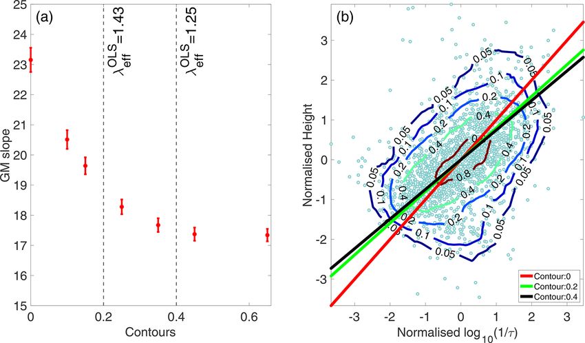
4158                                                                         E. Sarkar et al.: Temperature at meteor peak heights

half-amplitude decay time (τ ) as                                       to ambipolar diffusion, whereas at lower altitude, decay time
                                                                        tends to decrease due to additional effect of electron loss by
            T2  λ2 ln 2                                                 recombination and attachment (Younger et al., 2008). In ad-
Da = Kamb      = r 2 .                                            (2)
            P   16π τ                                                   dition, other geophysical factors, such as meteor fragmen-
                                                                        tation, turbulence within trail, chemical composition of the
Kamb in Eq. (2) is a constant related to the ionic constituent
                                                                        meteors or the temperature variation due to passage of tides
of the plasma in the trail (Hocking et al., 1997). The pressure
                                                                        and gravity waves, can contribute to the measurements of de-
at a given height (h) is
                                                                        cay time and heights at all altitudes (Hocking, 2004).
                  Rh mg
                  0 kT (z) dz
                                                                           Temperature estimation from meteor radar (MR) data re-
P (h) = P (0)e−                 ,                                 (3)   quires obtaining the best-fit regression line in the scattered
where m is the mass of a typical atmospheric molecule, g is             plot of log10 (1/τ ) and height. However, the pioneer work
the acceleration of gravity, k is the Boltzmann constant and            done by Hocking (1999) to implement this method using
z is an axis along the vertical. Substituting the equation for          ordinary least-squares fitting showed a clear systematic off-
pressure in Eq. (2) and differentiating Eq. (4) provides the            set between the MR temperature and co-located lidar mea-
height profile of the decay time:                                       surements, indicating that the estimated slope was not deter-
                                                                        mined correctly. To correct for this offset, a common practice
                                             Zh                         is to calibrate the meteor radar temperatures using tempera-
                                        mg          1                   tures from lidar, OH spectrometer, satellite or rocket clima-
log10 Da (h) = 2log10 T (h) + log10 e                   dz + 9,   (4)
                                         k        T (z)                 tology. Hocking et al. (2001b) provided a statistical compar-
                                             0
                                                                        ison technique (SCT) to calibrate the biased slope estimate
                                                                      as
 d           1                dT 1               mg 1                                 sδ
   log10           = 2log10 e          + log10 e          ,       (5)     d
                                                                        βOLS   = 1−         βSCT                                   (7)
dh         τ (h)              dh T (h)            k T (h)
                                                                                       sd
where 9 is a constant. Equation (5) states that the height              or
profile of decay time is a function of both temperature and                       sε  h
temperature gradient under the assumption of ambipolar dif-             βSCT = 1 −     βOLS ,                                        (8)
fusion for underdense meteor trails. In practice, most trail                       sh
echoes are received at a small altitude range referred to as the        where sδ and sε are the error variances of the (log of) dif-
region of peak meteor occurrence (Hocking, 1999). Hence                 fusion coefficient (or decay time) and height respectively, sd
a height-averaged temperature gradient near the peak height             and sh are data variances of log10 (1/τ ) and of height respec-
can be used to estimate the mean temperature (T0 ) at the peak                       d
                                                                        tively and βOLS           h
                                                                                           and βOLS   are slope coefficients when diffu-
height by fitting a linear function (Hocking, 1999). A linear           sion coefficient or height is treated as an independent variable
approximation of Eq. (5) is                                             respectively in the OLS regression analysis. The calibrated
          dT    mg                                                    slope, βSCT , is traditionally obtained by arbitrarily choosing
T0 = β 2 <    >+      log10 e,                                    (6)   sδ or sε that gives the best temperature estimates of MR as
           dh     k
                                                                        compared to optical or satellite data (e.g. Holdsworth et al.,
where β is the slope of the scattered plot of log10 (1/τ ) and          2006; Hocking et al., 2007; Kim et al., 2012). A severe short-
height, and T0 is the average temperature of the atmosphere             coming of such a calibration procedure is that the calibration
at the height of peak meteor occurrence. A typical scattered            factors (sδ and sε ) in the parentheses of Eq. (7) or Eq. (8) are
plot of height and log10 (1/τ ) shows significant variation in          dependent on the data selection criteria (e.g. limiting heights,
the measured data along both abscissa and ordinate (Fig. 1).            decay time or zenith angle to a certain range). Moreover, the
Traditionally, the slope (β) is estimated using the ordinary            outcome of any such calibration routine will depend on the
least-squares (OLS) method with log10 (1/τ ) as the indepen-            location of the MR and the choice of the calibration instru-
dent variable. The justification of using log10 (1/τ ) as an in-        ment. From a pure statistical context, the arbitrary choice of
dependent variable is that the measurement errors in τ are              calibration parameters makes the estimated temperature also
smaller than those in heights (Hocking et al., 1997). While             an arbitrary quantity, thereby making it impossible to draw
the pulse length and angular resolution, etc. of the radar in-          any reasonable statistical inferences.
troduces intrinsic measurement errors in heights, much of the              In practice, the ordinary least-squares method will not be
variation in decay time is due to various geophysical effects           valid for MR data since neither the height nor the decay time
that persist at all altitudes. At higher altitude, the collision        can be predetermined as an independent variable, and both
frequency with neutrals is reduced, and the diffusion is inhib-         variables are subject to intrinsic measurement errors and var-
ited in a direction orthogonal to the geomagnetic field (Jones,         ious geophysical effects. The reasons for such a bias, and
1991; Robson, 2001). This anisotropic diffusion causes an               thus the need for calibration, are discussed on theoretical and
increase in the duration of meteor radar echoes as compared             experimental grounds in Sect. 3.1. In addition, a statistical

Atmos. Meas. Tech., 14, 4157–4169, 2021                                                  https://doi.org/10.5194/amt-14-4157-2021
E. Sarkar et al.: Temperature at meteor peak heights                                                                                 4159

Figure 1. (a) Typical scatter plot of log10 (1/τ ) and height. The lines correspond to best-fit models using different regression methods
described in the text. The green and blue line corresponds to the ordinary least-squares method (OLS), with log10 (1/τ ) and height as
independent variables respectively. The red line corresponds to the geometric mean (GM) of βOLSd        h . (b) The bivariate distribution
                                                                                                   and βOLS
of the data. The measured height and log10 (1/τ ) are converted to dimension-free coordinates using Eq. (18). The relative density contours
are obtained by counting the number of detections in a circle of unit area relative to the detection density at the height of peak meteor
occurrences at the centre.

procedure to estimate sδ and sε using SCT calibration is for-           meteor trails are within the height of 70 to 110 km for unam-
mulated and presented in Sect. 3.1. An alternative method               biguous detections. Uncertainty in the height is ±1 km (or
that includes measurement errors in the regression model is             better for large zenith angle), which is determined by the
introduced in Sect. 3.2. This analysis does not require an ab-          2 km range resolution. In addition, the half-time (τ ) of the
solute knowledge of sδ or sε , but only the relative value is           received signal is calculated from the width of the autocorre-
needed. As an alternative to SCT calibration, in Sect. 4, an            lation function. A detailed description of the algorithm of the
independent slope estimation is obtained using the errors-in-           SKiYMET signal processing software is outlined in Hocking
variables model. A comparison study of the estimated MR                 et al. (2001a).
temperatures with co-located lidar temperatures is discussed               SGO is located at the corrected geomagnetic latitude of
to validate the method.                                                 64.1◦ , which is statistically a region of the auroral oval.
                                                                        Hence the radar frequently detects non-meteor targets during
                                                                        substorms associated with ionospheric plasma waves gener-
2   Instrumentation and data                                            ated due to Farley–Buneman instability (Kelley, 2009). The
                                                                        Doppler velocity of such echoes can be more than a few
The All-Sky Interferometric Meteor Radar (SKiYMET)                      hundreds of metres per second, which are mostly detected
at Sodankylä Geophysical Observatory (SGO; 67◦ 220 N,                   at low elevation (Lukianova et al., 2018). For the Sodankylä
26◦ 380 E; Finland) has been routinely monitoring daily                 radar, Kozlovsky and Lester (2015) identified ground echoes
meteor-height averaged temperatures and wind velocity since             modulated by the ionosphere during pulsating auroras. These
December 2008 (Kozlovsky et al., 2016). The radar oper-                 targets have near-zero Doppler velocities and are also ob-
ates at a transmission power of 15 kW and frequency of                  served at low elevation. Furthermore, the SKiYMET system
36.9 MHz, with a transmitting antenna which has a broad                 detects both underdense and overdense echoes as valid mete-
radiation pattern designed to illuminate a large expanse of             ors. However, more than 95 % of detections are underdense
the sky. The meteor trails are detected within a circle of              (Hocking et al., 2001b). The percentage of overdense trails
300 km diameter around SGO. The phase differences in the                may be larger during some meteor trails such as Geminids
five-antennae receiving array allow for the determination of            or Quadrantids, and this leads to underestimation of temper-
the azimuth, elevation, range, and line-of-sight Doppler ve-            atures (Kozlovsky et al., 2016). This artefact in temperature
locity of the meteor trails. The 2144 Hz pulse repetition fre-          was found to be reduced for Sodankylä radar for a zenith an-
quency of MR transmission introduces a range ambiguity of               gle of less than 50◦ . The initial data selection criteria is kept
70 km, and the built-in analysis software therefore assumes

https://doi.org/10.5194/amt-14-4157-2021                                                   Atmos. Meas. Tech., 14, 4157–4169, 2021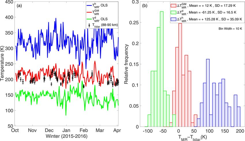
4160                                                                     E. Sarkar et al.: Temperature at meteor peak heights

to a bare minimum, such that all heights and decay times are       3     Method: regression analysis
included, as long as they are unambiguous detections above a
40◦ elevation angle with Doppler radial velocity in the range      3.1    Estimation of error variances in decay time and
±100 m s−1 . Subsequently, to improve the temperature esti-               height
mation, we used a contour selection process; i.e. the data out-
side a certain contour in the normalised height–log10 (1/τ )       In the following text we use the notation and formulation
distribution were rejected (Fig. 1b).                              in Gillard and Iles (2005). The observables, log10 (1/τ ) and
   For temperature estimation we considered daily data for         height, are represented as di and hi respectively and the cor-
a 6-month period from October 2015 to March 2016 since             responding unobserved true values as ξi and ηi respectively,
simultaneous lidar measurements were available during this         where the index i represents the ith meteor detection. For
time. The Compact Rayleigh Autonomous Lidar (CORAL)                consistency we also assume that log10 (1/τ ) is presented in
provided vertical profiles of the atmospheric temperature at       abscissa, and height is in the ordinate in the respective scat-
27–98 km over Sodankylä as part of the GW-LCYCLE-II                tered plot (as shown in Fig. 1). Suppose we are assuming a
(Gravity Wave Life Cycle Experiment) campaign in winter            linear relation in variables ξi and ηi as
2015/2016 (Reichert et al., 2019). The median number of            ηi = α + β ξi , i = 1, 2, . . ., N.                        (9)
daily meteor detections in this data set is 1652, with a mini-
mum of 410 meteor detections on 4 October 2015 and a max-          Due to measurement errors and various geophysical pro-
imum of 3456 detections during the Geminids meteor shower          cesses, the true values ξi and ηi will be subject to random
on 14 December 2015.                                               errors, and hence the observable di and hi will have scatter
   The Mass Spectrometer–Incoherent Scatter or MSIS90              around the linear model in Eq. (9):
(Hedin, 1991) model temperatures are used to generate a
temperature gradient model near the peak heights. Model            di = ξi + δi                                              (10)
temperatures are computed for each date at intervals of 6 h        and
between 85 and 95 km. A third-degree polynomial fit is car-
ried out to obtain the height profiles at 06:00, 12:00, 18:00      hi = ηi + εi = α + β ξi + εi ,                            (11)
and 24:00 UT. For each time interval, the gradient at the re-
spective meteor peak height, as well as at 1 km above and          where δi and εi are errors in the measured log10 (1/τ ) and
below the peak height, is estimated. These 12 values are then      height respectively and are assumed to be mutually uncor-
used to obtain the mean and standard deviation of the tem-         related, have zero mean and be independent of the suffix i.
perature gradient for each day near the peak height, which         This implies that the measurement error variances, sδ and sε ,
varies in the range 89 ± 1 km. The daily meteor detections,        are constant with respect to the suffix i. Classical regression
the peak heights and the corresponding temperature gradient        analysis or ordinary least-squares (OLS) treats di as an in-
model values are shown in Fig. 2. The standard deviation of        dependent variable without intrinsic errors (or, di = ξi ) and
the MSIS model values corresponds to roughly of the order          then minimises the sum of squared residuals along the or-
of 0.7 K km−1 .                                                    dinate. The slope from the OLS method can be represented
   Our reasons for choosing the MSIS temperature gradient          in terms of the covariance (Cov) and variance (Var) as (e.g.
are twofold. Firstly, MSIS data are easily accessible from the     Smith, 2009; Keles, 2018)
online version, which guarantees reproducibility of this work                                 √
                                                                     d      Cov(di , hi )       sh
independent of location. Secondly, even if the temperature         βOLS  =                ≡r √ ,                              (12)
                                                                              Var(di )          sd
gradient term in Eq. (6) is ignored, the resulting offset in the
estimated temperature is on average 10 % (Hocking, 1999) or                 d
                                                                   where βOLS     is the OLS slope estimated by considering
less. Hence an approximate estimate is sufficient for the main     log10 (1/τ ) as an independent variable, and r is the Pear-
objective of this paper. However, the actual temperature gra-      son product-moment correlation coefficient between d and
dient in the atmosphere may be slightly different from these       h. Likewise, by reversing the arguments above, it is trivial to
model values, which can contribute to the biasing effect in        show that the reciprocal value of the OLS slope estimate with
the estimated temperatures. Any such possibility and its ef-       height as an independent variable is (e.g. Smith, 2009)
fect on the estimated temperatures is addressed in the subse-                                  √
quent section.                                                       h        Var(hi )      1 sh
                                                                   βOLS  =                ≡ √ .                              (13)
                                                                            Cov(di , hi )   r    sd
                                                                   To see the effect of errors in the independent variable on the
                                                                                                   d , Eqs. (10) and (11) are used
                                                                   OLS slope estimate, e.g. for βOLS
                                                                   in Eq. (12):

                                                                    d        Cov(ξi + δi , α + β ξi + εi )
                                                                   βOLS =                                  .                 (14)
                                                                                    Var(ξi + δi )

Atmos. Meas. Tech., 14, 4157–4169, 2021                                              https://doi.org/10.5194/amt-14-4157-2021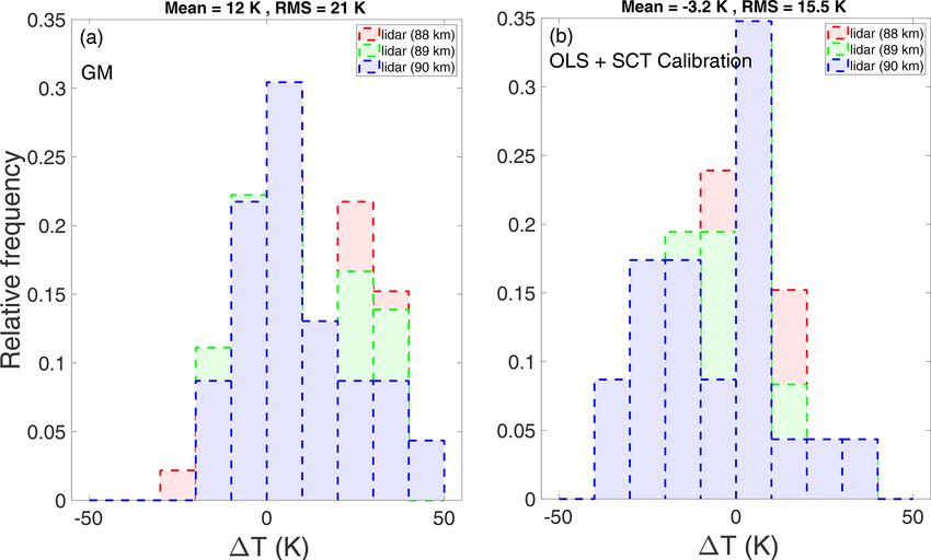
E. Sarkar et al.: Temperature at meteor peak heights                                                                                 4161

Figure 2. (a) Temperature gradient model derived from MSIS90. (b) Peak meteor heights for the data used in this work and (c) the daily
meteor detection for zenith angle less than 50◦ and velocity in the range ±100 m s−1 .

Since δi , εi and ξi are mutually independent, Eq. (14) sim-         The corresponding biased temperatures, TMR    d and T h re-
                                                                                                                            MR
plifies to                                                           spectively, are estimated using Eq. (6). Experimental values
                                                                     of the parameters sδ and sε can be obtained by comparing
 d       β Cov(ξi , ξi )       1                                     these estimated biased temperatures with the co-located lidar
βOLS =                   =     Var(δi )
                                        β = ζ β,            (15)
         Var(ξi + δi )     1 + Var(ξi )                              temperatures (Tlidar ) as the reference values. Using Eqs. (7)
                                                                     and (8), and noting that the slope is proportional to the esti-
where ζ is known as the attenuation or regression dilu-              mated temperatures from Eq. (6), we obtain
tion bias. Since variances are always positive by definition,
Eq. (15) shows that in the presence of measurement error                    T            d                  T h − T
                                                                                 lidar − TMR

                                                                                                                MR     lidar
in the so-called independent variable (in abscissa), the OLS         sδ ≈                       sd and sε ≈         h
                                                                                                                                 sh , (17)
                                                                                   Tlidar                          TMR
                   d ) will always be smaller than the un-
slope estimate (βOLS
                             h
biased slope β. Likewise, βOLS   is greater than β if there is                d and T h are MR temperatures estimated using
                                                                     where TMR         MR
error in the measured height (specific example presented in          OLS fitting with log10 (1/τ ) and height as an independent
Fig. 1a). By substituting di = ξi + δi , Eq. (15) can be rear-       variable respectively. Furthermore, if the measurements are
ranged as                                                            normalised with the mean and standard deviation (SD) as

  d            Var(δi )                                                       di − mean(di )            hi − mean(hi )
βOLS  = 1−                β.                              (16)       di 0 =        √         and hi 0 =      √         ,              (18)
               Var(di )                                                             sd                         sh

Equation (16) is a well known identity in statistical literature     then Var(di 0 ) = Var(hi 0 ) = 1, and the OLS estimate of the
(e.g. Carroll and Ruppert, 1996; Frost and Thompson, 2000),          ratio of the measurement error variance is (from Eqs. 17
that was re-derived by Hocking et al. (2001b) in Eq. (7) in the      and 18)
context of SCT correction. Equation (16) reveals that an ab-
solute knowledge of error variances, sδ ( or sε ), is required to                sε0   T h − Tlidar Tlidar
                                                                     λOLS
                                                                      eff =           ≈ MR          · h ,                             (19)
obtain the bias-corrected slope (β) if we choose OLS fitting                     sδ 0            d
                                                                                       Tlidar − TMR  TMR
for the slope estimate. A common practice is to calibrate the
biased slope with optical or satellite data by arbitrarily choos-    where the error variances, sε0 and sδ 0 , are in the dimension-
ing a value of sδ or sε (e.g. Holdsworth et al., 2006; Hocking       free system defined by Eq. (18). In essence, λOLS eff is a mea-
et al., 2007; Kim et al., 2012). In the remaining part of this       sure of all sources of errors in the normalised heights and
section, we demonstrate how to obtain an average value of            decay times that cause the real data to deviate from the ide-
the error variances in these data following a revised calibra-       alised physical model of Eq. (6), thereby producing a typical
tion procedure.                                                      scatter as seen in Fig. 1.
   For each 24 h of the data set, we performed two OLS fit-             λOLS
                                                                         eff , sδ and sε were estimated by Eqs. (17) and (19) us-
                    d
tings to estimate βOLS         h
                         and βOLS  by using Eqs. (12) and (13).      ing 24 h of MR data and co-located lidar temperatures at 88,

https://doi.org/10.5194/amt-14-4157-2021                                                    Atmos. Meas. Tech., 14, 4157–4169, 2021
4162 E. Sarkar et al.: Temperature at meteor peak heights
Figure 3. (a) Temperature estimated in OLS method using log10 (1/τ ) (green) and height (blue) as an independent variable. Also shown are
(red) the temperatures obtained using the geometric mean (GM) fitting and the lidar temperatures (in black). (b) The offset between the lidar
(Tlidar ) temperatures and the estimated MR temperatures (TMR ) using OLS fitting and GM fitting (without contour selection).
89 and 90 km for the dates for which lidar data were avail- can easily skew the distribution in this direction. On the other
able. The biasing effect on the OLS estimate of MR tem- hand, natural geophysical variability in these data contributes
peratures with log10 (1/τ ) and height as an independent vari- significantly at all altitudes. As seen in Table 1, the aver-
able respectively are presented in Fig. 3 (green and blue lines age error in height for contour levels 0, 0.2 and 0.4 are 5.0,
and histogram). As expected from Eq. (7) or Eq. (8), a mean 3.0 and 2.2 km respectively. This error is significantly higher
offset of −75 and +335 K occurs depending on whether than what is expected from purely parameter estimation er-
log10 (1/τ ) or height respectively is considered as an inde- ror (for zenith angle less than 50◦ , the error in height is 1 km
pendent variable. In practice, the magnitude of these biases or less), indicating that geophysical variability dominates the
is related to the total errors in heights and log10 (1/τ ) from total error variance in these data at all altitudes. The aver-
Eq. (17), which was not taken into account by the OLS re- age error variances estimated at the contour level 0.2 (Ta-
gression model in Eqs. (12) and (13). Furthermore, the rel- ble 1) correlate very well with the values reported in Hock-
ative density contour lines for each data point is obtained ing (2004) and Holdsworth et al. (2006). Hocking (2004) es-
by counting the number of detections in a circle of unit timated 4(height) = 3.25 km using a numerical model for a
area in the normalised height–log10 (1/τ ) plane relative to pulse length equivalent to 2 km and a meteor at an altitude
the number of detections in unit area at the peak meteor re- of 90 km and zenith angle 50◦ . Likewise, their estimation
gion (Fig. 1b). In addition, all the error estimates from the of 4log10 (1/τ ) = 0.14 was based on simulation studies for
SCT method are obtained at contour levels 0, 0.2 and 0.4, meteors below 95 km and confirmed that “decay times’ vari-
and the results are presented in Table 1. Several key features ability” arise due to 27 % variability in Kamb and 8 % vari-
of these data are reflected in Table 1. Despite the data trans- ability in temperatures over the meteor region. The argument
formation via Eq. (18), the average error variances for the for choosing 95 km as the maximum height is that above
height data are more than those for the log10 (1/τ ) data in this altitude, meteor decay rates are substantially affected by
these coordinates. This asymmetry in the error variances im- processes other than ambipolar diffusion. Holdsworth et al.
plies that the bivariate distribution is slightly skewed away (2006, p. 5) applied similar data rejection criteria and found
from a perfectly normal distribution along the y direction. out that 4log10 (1/τ ) = 0.14 is required to calibrate the slope
However, this effect of asymmetric error variances is less if log10 (1/τ ) is used as an independent variable in the OLS
pronounced near the core of this distribution. This implies regression model. Likewise, Thorsen et al. (1997) performed
that the parameter λOLS
eff is closer to 1 near the core of this the comparison between the parameter estimation error and
distribution and further away from 1 near the tail of the dis- the geophysical variability for estimating the mean wind field
tribution. The data near the outer contour area are subject to in the middle atmosphere and found that the geophysical
larger parameter estimation error due to observational limita- variability dominated at all heights.
tion. For example, the zenith-angle-dependent error in height
Atmos. Meas. Tech., 14, 4157–4169, 2021 https://doi.org/10.5194/amt-14-4157-2021E. Sarkar et al.: Temperature at meteor peak heights 4163
Table 1. The average value of the (square root of) error variances in 3.2 Errors-in-variables (EIV) model: GM solution
height and log10 (1/τ ); sε0 and sδ 0 are given along with the average
value of λ from SCT calibration (λOLS eff ) at contour levels 0, 0.2 and For fitting a straight line model, such as
0.4 for winter 2015–2016.
y(x) = a + bx (20)
Contour: 0 0.2 0.4
√ to a set of N data points (xi , yi ) measured with errors, the
sε /km 5.0 3.0 2.2
√ corresponding χ 2 merit function is (Press et al., 1992, p. 660)
sδ /s−1 0.18 0.14 0.11
< sε 0 > 0.62 0.44 0.38 N
< sδ 0 > 0.37 0.31 0.30
X (yi − a − bxi )2
χ2 = , (21)
< λOLS
eff > 1.68 1.43 1.25 i=1
2 + b2 σ 2
σyi xi
where σyi and σxi are the standard deviation of the ith data
It is worth noting that instead of directly using the indi- point, and the weighted sum in the denominator of Eq. (21)
vidual observation between biased MR temperatures and li- can be interpreted as the weighted error of the ith data point.
dar measurements from Eq. (17), we have used the statistical The regression coefficients, a and b, can be found by min-
mean of differences for calibration. This is because lidar data imising the merit function with respect to these coefficients
are not available for all days during the 6 months of data used following any suitable numerical root-finding routine. How-
in this work. Moreover, both MR and lidar data have their ever, under the assumption of symmetric error variances, it
own intrinsic errors and technical differences in the observa- is possible to derive an analytic solution for the regression
tion time and volume of sky. MR temperatures are daily aver- coefficients. This solution, when the data are appropriately
ages over 24 h of observation, whereas lidar data are just the normalised, leads to a slope estimate which is both scale-
nightly mean profile. The lidar probes a small volume limited invariant and symmetric with respect to the data.
to the diameter of the lidar beam, while the radar illuminates Application of Eq. (21) to physics data requires that all
a large part of the sky. For a single observation, the lidar may measured variables are dimensionally consistent so that χ 2
see the phase structure of large-scale gravity waves, while is dimension-free. Moreover, the analysis in this section re-
the MR averages over the gravity wave structure due to dif- quires that the measurements are presented in an appropriate
ferent spatial resolutions. As a result, the radar averages over dimension-free system. This facilitates the direct comparison
gravity waves with horizontal wavelengths smaller than few between different parameters, such as the measured variables
hundred kilometres. On the other hand, the lidar may resolve or the associated error variances. By applying the coordinate
these gravity waves if the runtime is shorter than the period transformation introduced in Eqs. (18) to (9), we therefore
of these waves. As gravity wave amplitudes can be up to 10– intend to solve the simplified bivariate linear system of equa-
15 K at these altitudes (Reichert et al., 2019), we cannot ex- tions,
pect perfect agreement between radar and lidar temperature √
sd
due to geophysical variation which shows up differently in ηi 0 = β √ ξi 0 ≡ βW ξi 0 , (22)
sh
the two data sets as a result of the different observational
volumes. where ηi 0 , ξi 0 and βW are dimension-free. For the specific
While such calibration routine may prevent large offsets in choice of normalisation by Eq. (18), the intercept (αW ) is
the estimated temperatures, the day-to-day variation in these always zero in the transformed coordinate system. The merit
error variances due to natural geophysical processes will per- function in Eq. (21) can be further simplified by invoking
sistently introduce artefacts in the estimated temperatures. a homoscedastic standard weighting model (Macdonald and
Moreover, due to the continually changing atmospheric dy- Thompson, 1992). This error model assumes that the error
namic, these calibration parameters need to be updated at variances are independent of data point, thereby simplifying
time intervals. This in turn requires availability of optical the merit function as (Macdonald and Thompson, 1992; Lolli
or satellite data throughout the year for the given location. and Gasperini, 2012)
In all generality, it is desirable to avoid any kind of calibra-
tion process and instead formulate an independent estimate N
X (hi 0 − βW di 0 )2
of temperatures using MR data alone. As an alternative to χ 2 (βW , αW = 0) ≡ 2 )
, (23)
the OLS method, errors-in-variables (EIV) regression analy- i=1 sδ 0 (λ + βW
sis provides a way to incorporate the error variances in both
where sδ 0 and sε0 are constant error variances of the mea-
height and log10 (1/τ ) data, thereby reducing the biasing ef-
sured log10 (1/τ ) and heights respectively in the normalised
fect in the estimated slope parameter.
(or, dimension-free) coordinate system, and λ is the ratio
sε0
λ= . (24)
sδ 0
https://doi.org/10.5194/amt-14-4157-2021 Atmos. Meas. Tech., 14, 4157–4169, 20214164 E. Sarkar et al.: Temperature at meteor peak heights
The χ 2 minimisation of Eq. (23) with respect to βW leads to and symmetric in the variables (e.g. Ricker, 1984; Smith,
the analytic expression (Carroll and Ruppert, 1996; Smith, 2009). While these properties do not necessarily imply that
2009; Lolli and Gasperini, 2012) for the EIV slope parameter the GM solution is the correct solution (discussed below),
in terms of the variances (sd0 , sh0 ) and covariances (sh0 d0 ) of this first estimate reflects the nature of the biasing effect in
the measured variables, the estimated slope in relation to the data selection process.
q A specific example of GM fitting is presented in Fig. 1a. The
sh0 − λsd0 + (sh0 − λsd0 )2 + 4λsh20 d0 standard error in the OLS and GM slope estimate reported in
βW = (25) Fig. 1a is from Vicente de Julián-Ortiz et al. (2010). Due to
2sh0 d0
the relatively low detections with Sodankylä radar (Fig. 2c),
or the 2σ error in the estimated temperature using the GM so-
lution is found to be significantly higher (13 K on average at
q
1 − λ + (1 − λ)2 + 4λsh20 d0
βW ≡ . (26) contour level 0). This 13 K of√ noise √
level in the temperature
2sh0 d0 can be reduced by a factor of 3 or 5 if a 3 or 5 d running
mean of temperature is estimated with this radar. However,
since sd0 = sh0 = 1 from Eq. (18). And the covariance (sh0 d0 )
to test the robustness of the proposed method, this paper has
is computed using the standard definition,
estimated the daily averaged temperatures.
1 XN The systematic offset between MR temperature and co-
sh0 d0 = (hi 0 di 0 ), for large N. (27) located lidar temperature as a result of using Eq. (30) is re-
N i=1
flected in Fig. 3a (red curve) and b (red histogram). Each
Equation (26) can be solved if a prior knowledge of λ is avail- of these temperatures are then compared with lidar temper-
able, which in turn requires a precise estimate of all sources atures at 88, 89 and 90 km for the dates when lidar data are
of errors in the measured data. In the more practical case for available. The intrinsic noise in the lidar temperature is about
unknown λ, we need to initiate a good starting estimate. Us- 5–10 K (Reichert et al., 2019), which implies no temperature
ing the calibration procedure described by Eqs. (17) and (18), gradient is observed between 88 and 91 km in these data. Fig-
the mean values of sε0 and sδ 0 are found to be 0.62 ± 0.04 and ure 3b (red histogram) reveals that the MR temperatures are
0.37 ± 0.06 respectively (without any contour selection: Ta- overestimated by a mean value of +58 K for the case of the
ble 1). Since the EIV estimate of the slope requires only the GM solution.
ratio between sε0 and sδ 0 , a good choice of this starting value When compared to the temperature gradient model de-
is λ = 1. Furthermore, for λ = sε0 = sδ 0 = 1, there is a sim- rived from optical, satellite and rocket climatology (e.g.
ple geometric interpretation of the merit function in Eq. (23). Holdsworth et al., 2006), it can be easily argued that our
This solution corresponds to minimising the Euclidean or or- MSIS-derived gradient model (Fig. 2a) is more negative than
thogonal distance between the fitted line and the measured expected. If these values are shifted by a constant positive
data. The residual function to be minimised with respect to offset of +1 K km−1 , the absolute value of the estimated tem-
the regression coefficients is peratures will increase by 10 K (Singer et al., 2004). This will
further increase the offset between lidar and MR tempera-
N N ture, thereby shifting the histogram (in red) in Fig. 3b further
X (hi 0 − βW di 0 )2 X (hi 0 − di 0 )2
χ2 = 2
≡ (28) to the right.
i=1 1 + βW i=1
2
On the other hand, lidar temperatures are usually obtained
since βW = 1 when λ = 1 from Eq. (26). Following Eq. (22), during the night-time, which can lead to a systematic offset
we therefore have our first estimate of β in the scattered plot due to day–night differences or tidal variations. As discussed
of log10 (1/τ ) and heights, by Hocking et al. (2004), the day–night temperature differ-
√ ence at these altitudes is of the order of 3–4 K. This is sig-
sh nificantly less than the standard errors in these temperatures,
β=√ . (29)
sd which is on average 6 K at contour level 0. Hence we ex-
pect the day–night difference in Sodankylä MR temperatures
Equation (29) is commonly referred to as a reduced major to be insignificant during the winter period. Moreover, any
axis (RMA) solution in statistics literature (Smith, 2009). In attempt to estimate MR temperatures using only night-time
practice, this is just the geometric mean (GM) of the two data has the adverse effect of reducing the accuracy in the
OLS estimates, βOLSd h , as can be seen by combining
and βOLS estimated temperatures due to data loss. While no specific
Eqs. (12) and (13): studies of tidal variation have been made for this location,
√ the data from other sites (e.g. Hocking and Hocking, 2002;
sh
q
d h
βGM = βOLS βOLS ≡ √ . (30)
sd Stober et al., 2008) show that the temperature variation due to
tidal activity is typically less than 10 K. We can therefore rule
The GM solution in Eq. (30) has the unique feature that this out the possibility of an offset in the MSIS gradient model or
is the only case of EIV estimate which is both scale-invariant
Atmos. Meas. Tech., 14, 4157–4169, 2021 https://doi.org/10.5194/amt-14-4157-2021E. Sarkar et al.: Temperature at meteor peak heights 4165
tidal effects as the primary cause for the +58 K offset seen in peak meteor counts. The mean difference between lidar and
Fig. 3b (red histogram). MR temperatures is +12 K, which is expected due to the vari-
Ricker (1984) emphasised that the biasing in GM solution ation in the true value of λ from 1. The root-mean-square
is conditional upon the value of the correlation coefficient (rms) difference is about 21 K. This difference is partly due
(r) between the variables, while Kimura (1992) demonstrated the intrinsic errors of 5–10 K in lidar temperature and partly
that this solution will be an overestimate in the case of low due to the statistical noise in the estimated MR temperatures.
r values. For the data set used in this work, we found that For direct comparison with the results above, we have also
the correlation between log10 (1/τ ) and height is typically estimated the MR temperatures using the revised SCT cali-
0.50±0.05, thereby indicating the presence of significant nat- bration procedure described in Sect. 3.1. For this we have es-
ural variation in the measurements. Furthermore, Jolicoeur timated the OLS slope (βOLS d ) and used √s = 0.11 (Table 1)
δ
(1990) used error modelling to conclude that r must be more to obtain the calibrated temperatures from Eqs. (16) and (6).
than 0.6 for the GM solution to be acceptable. In fact, we These calibrated temperatures are presented in Fig. 5. The
have observed that if we restrict our data selection process by histogram in Fig. 6b shows the differences between lidar data
excluding all data beyond the density contour 0.2 (Fig. 1b), and the SCT-calibrated MR temperatures. The mean differ-
this increases the r to be typically around 0.66 ± 0.06, with ence between the MR and lidar temperatures is again about
the consequence of reduced biasing in the GM solution. Such −3 K, thereby showing that the biasing effect has been prop-
a contour selection process essentially removes the erroneous erly corrected by this calibration procedure. The rms differ-
data at higher and lower altitudes from the tail of the distri- ence is 15 K. Although the temperature estimated from the
bution, whereby the assumption of equal error variances (i.e. GM solution is slightly biased as compared to that estimated
sε0 ≈ sδ 0 ) is achieved in the normalised coordinates (Table 1). using SCT calibration, the presence of artefacts in the latter
In other words, the validity of GM solution is conditional is clearly visible in Fig. 5. As evident from Fig. 7, the GM so-
upon how close the parameter λ is to 1 for a given data selec- lution based on contour selection improves the temperature
tion process. estimation significantly as compared to the traditional use of
the OLS regression analysis.
The EIV analysis does not distinguish between the mea-
4 Results and discussion surement error and natural geophysical variability (e.g.
Sprent, 1990, p. 13). In other words, the error variances, sδ 0
The convergence of λ towards 1 near the core of this bivari- and sε0 , consist of both measurement errors and the natu-
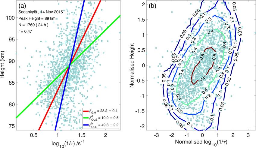
ate distribution is evident from Table 1. This is demonstrated ral geophysical variation. The effective value of λ in a nor-
in Fig. 4a, where we have estimated the GM slope at vari- malised coordinate may vary on a day-by-day basis and may
ous contour levels between 0 and 0.7. In addition, Fig. 4b be radar-dependent. For example, meteor trails can get mod-
reflects the asymptotic behaviour of GM solution at higher ified by wind effects, ion composition, meteor fragmentation
contour levels in normalised coordinates. For these data, be- and strong ionospheric currents, as well as temperature and
yond the contour level 0.4, any change in slope at higher con- pressure fluctuations, on various spatial and temporal scales
tour level is within the 2σ error limit. This error in the slope (Hocking, 2004; Younger et al., 2014). Despite the contour
corresponds to an average 2σ error of 11 K in the estimated selection process, asymmetric effects of geophysical varia-
temperatures at contour level 0.4. In addition, the estimated tion may have increased the effective variance of hi 0 , leading
temperatures can be biased due to small variation of λ from to overestimates in the GM solution (Gillard and Iles, 2005).
1 on a day-by-day basis. For example, If the true value of Due to the high-latitude location of Sodankylä radar, the geo-
λ is 1.25, the GM slope will be overestimated by 4 % (from magnetic effect above 95 km can contribute to the systematic
Eq. 26 for the date 14 November 2015). For a typical win- bias. Below 85 km, the decay of meteor radar echoes may
ter temperature of 200 K at 90 km, a 4 % offset translates to deviate slightly from diffusion-only evolution (Lee et al.,
overestimation of temperatures by 8 K. In principle, this bias 2013), thereby requiring a better physical model that does not
can be further reduced by selecting a higher contour level assume the linearity of Eq. (6). Assessing the contribution
than 0.4, with the consequence of increased noise level in the of geophysical variability at various altitudes would require
estimated temperatures. For these data, the contour level 0.4 carefully designed replicates of observations as well as long-
is found to provide an optimum condition such that a maxi- term comparison of MR temperatures with other co-located
mum of 25 % uncertainty in the parameter λ leads to 4 % bias instruments. In other words, the case for λ 6 = 1 needs to be
in temperature, which, in turn, is comparable to the standard handled with careful modelling of errors by taking into ac-
error in the temperature from regression analysis. count the dominant effect of geophysical variability in these
We have applied the GM slope estimate at contour level data. This remains a subject of future research.
0.4 to the MR data from the period October 2015 to March
2016. This is presented in Fig. 5, along with the data from
co-located lidar observations. The differences between MR
temperatures and lidar are shown in Fig. 6a for altitudes near
https://doi.org/10.5194/amt-14-4157-2021 Atmos. Meas. Tech., 14, 4157–4169, 20214166 E. Sarkar et al.: Temperature at meteor peak heights
Figure 4. GM solution at different contour levels in (a) original coordinate and in (b) normalised coordinate for the date 14 November 2015.
The vertical dashed lines in (a) correspond to the average value of λ obtained from SCT calibration at contour level 0.2 and 0.4 respectively
for winter 2015–2016. The error bar in (a) corresponds to 2σ error .
Figure 5. Comparison of the bias-corrected MR temperatures with lidar data for the winter 2015–2016. The solid line corresponds to the
temperature estimated using the GM solution at contour level 0.4. The dashed line corresponds to the SCT-calibrated temperatures using the
co-located lidar measurements. The OLS estimates are obtained with log10 (1/τ ) as an independent variable. The errors in lidar temperatures
are 5–10 K, and the 2σ error (grey shade) of the temperature from EIV analysis is on average 11 K. The differences between lidar and MR
temperatures are presented in Fig. 6.
5 Summary which is mainly due to the presence of various error terms.
We have reviewed the conventional calibration procedure (1)
The biasing effect in MR temperature has been a pressing is- and then provided an alternative method (2) for estimating
sue for the last 2 decades. Attempts have been made in the MR temperature that does not require any calibration. We
past to correct the slope in the scattered plot of log10 (1/τ ) have applied both of these methods to the MR data from win-
and height, usually either by direct calibration with optical ter 2015–2016 and assessed the quality of the estimated MR
or satellite data or by an arbitrary choice of data rejection temperature using co-located lidar measurements. The key
criteria to exclude parts of measurements. This paper has points from each of these two aspects of the paper are given
addressed the underlying reasons for such a biasing effect, below.
Atmos. Meas. Tech., 14, 4157–4169, 2021 https://doi.org/10.5194/amt-14-4157-2021E. Sarkar et al.: Temperature at meteor peak heights 4167
Figure 6. Difference between MR temperatures and lidar data for (a) the GM solution at contour level 0.4 and (b) SCT calibration applied
d . MR temperatures are shown in Fig. 5.
to OLS estimate of βOLS
Figure 7. (a) Improved temperature estimation using the GM solution (red) as compared to OLS estimates (blue and green) at contour level
0.4. (b) Reduced mean offset between MR and lidar temperature for GM slope estimate (red) as compared to OLS estimate (green and blue).
1. This paper has reviewed the statistical comparison tech- 2. As an alternative method, we have applied the errors-
nique (SCT), originally proposed by Hocking et al. in-variables (EIV) regression analysis to estimate the
(2001b), within the context of MR temperature cali- slope in the scattered plot of log10 (1/τ ) and height. The
bration. We have extended the theoretical basis of the model error in EIV analysis takes into account the total
SCT method to obtain an estimate of error variances of errors variances in both abscissa and ordinate. It is ob-
log10 (1/τ ) and height using co-located lidar measure- served that the geophysical variability dominates at all
ments. No significant offset was seen in the calibrated altitudes as compared to measurement errors and is the
MR temperature, even without applying any outlier re- key factor in addressing the biasing effect. Moreover,
jection criteria. But artefacts introduced due to the dif- any asymmetry in the error variance is minimal near the
ference in measurement techniques between MR and li- meteor peak region. This allows for an independent esti-
dar were clearly visible in the estimated temperatures. mate of weighted-averaged atmospheric temperatures at
90 km using a suitable contour selection procedure. The
https://doi.org/10.5194/amt-14-4157-2021 Atmos. Meas. Tech., 14, 4157–4169, 20214168 E. Sarkar et al.: Temperature at meteor peak heights
temperatures estimated using this method show very Chilson, P. B., Czechowsky, P., and Schmidt, G.: A compari-
good agreement with co-located lidar measurement and son of ambipolar diffusion coefficients in meteor trains using
with reduced systematic offset as compared to the tradi- VHF radar and UV lidar, Geophys. Res. Lett., 23, 2745–2748,
tional least-squares analysis. https://doi.org/10.1029/96GL02577, 1996.
DLR (German Aerospace Center): Lidar data, HALO database [data
sets], available at: https://halo-db.pa.op.dlr.de/mission/109, last
access: 17 May 2021.
Data availability. Data used in the paper are available at https:
Frost, C. and Thompson, S. G.: Correcting for regression dilution
//www.sgo.fi/pub/AMT_2020_ESarkar/ (last access: 13 April 2021,
bias: comparison of methods for a single predictor variable, J. R.
Sarkar et al., 2021, emranul.sarkar@oulu.fi). The MSIS model
Stat. Soc. A Stat., 163, 173–189, https://doi.org/10.1111/1467-
data were obtained from https://ccmc.gsfc.nasa.gov/modelweb/
985X.00164, 2000.
atmos/nrlmsise00.html (last access: 17 May 2021, Hedin, 1991,
Gillard, J. W. and Iles, T. C.: Method of moments estimation in
https://doi.org/10.1029/90JA02125). The lidar data are available at
linear regression with errors in both variables, Cardiff University
https://halo-db.pa.op.dlr.de/mission/109 (last access: 17 May 2021,
School of Mathematics Technical paper, Cardiff, Wales, UK, 3–
DLR, 2021).
43, 2005.
Hedin, A. E.: Extension of the MSIS thermosphere model into
the middle and lower atmosphere, J. Geophys. Res., 96, 1159–
Author contributions. ES developed the method, carried out all 1172, https://doi.org/10.1029/90JA02125, 1991 (data avail-
data analysis and wrote the manuscript. The idea was suggested able at: https://ccmc.gsfc.nasa.gov/modelweb/atmos/nrlmsise00.
by AK, who also supervised this work. TU prepared the script for html, last access: 17 May 2021).
reading the raw data files from the radar and supervises the doctoral Hocking, W. K.: Temperatures using radar-meteor de-
thesis of ES. IV co-supervises the doctoral thesis of ES and made cay times, Geophys. Res. Lett., 26, 3297–3300,
suggestions. BK provided the lidar data. ML supported the MR op- https://doi.org/10.1029/1999GL003618, 1999.
eration at the Sodankylä. All the authors contributed to proofreading Hocking, W. K.: Radar meteor decay rate variability and at-
the manuscript. mospheric consequences, Ann. Geophys., 22, 3805–3814,
https://doi.org/10.5194/angeo-22-3805-2004, 2004.
Hocking, W. K. and Hocking, A.: Temperature tides deter-
Competing interests. The author declares that there is no conflict of mined with meteor radar, Ann. Geophys., 20, 1447–1467,
interest. https://doi.org/10.5194/angeo-20-1447-2002, 2002.
Hocking, W. K., Thayaparan, T., and Jones, J.: Meteor de-
cay times and their use in determining a diagnostic meso-
Acknowledgements. Emranul Sarkar thanks the University of spheric temperature-pressure parameter: Methodology and
Oulu’s Kvantum Institute for their support. We thank the anony- one year of data, Geophys. Res. Lett., 24, 2977–2980,
mous referees for providing helpful suggestions to improve this pa- https://doi.org/10.1029/97GL03048, 1997.
per. Hocking, W. K., Fuller, B., and Vandepeer, B.: Real-time de-
termination of meteor-related parameters utilizing modern
digital technology, J. Atmos. Sol.-Terr. Phy., 63, 155–169,
Financial support. Ilkka Virtanen has been supported by the https://doi.org/10.1016/S1364-6826(00)00138-3, 2001a.
Academy of Finland (project no. 301542). Bernd Kaifler has Hocking, W. K., Thayaparan, T., and Franke, S. J.: Method for sta-
been supported by the German Research Foundation (DFG), re- tistical comparison of geophysical data by multiple instruments
search unit Multiscale Dynamics of Gravity Waves (MS-GWaves; which have differing accuracies, Adv. Space Res., 27, 1089–
grant no. RA 1400/6-1). Mark Lester has been supported by the 1098, https://doi.org/10.1016/S0273-1177(01)00143-0, 2001b.
Science and Technologies Facilities Council (STFC; grant no. Hocking, W. K., Singer, W., Bremer, J., Mitchell, N., Batista, P.,
ST/S000429/1). Clemesha, B., and Donner, M.: Meteor radar temperatures at
multiple sites derived with SKiYMET radars and compared to
OH, rocket and lidar measurements, J. Atmos. Sol.-Terr. Phy.,
Review statement. This paper was edited by Jorge Luis Chau and 66, 585–593, https://doi.org/10.1016/j.jastp.2004.01.011, 2004.
reviewed by two anonymous referees. Hocking, W. K., Argall, P. S., Lowe, R. P., Sica, R. J., and Elli-
nor, H.: Height-dependent meteor temperatures and comparisons
with lidar and OH measurements, Can. J. Phys., 85, 173–187,
https://doi.org/10.1139/p07-038, 2007.
References Holdsworth, D. A., Morris, R. J., Murphy, D. J., Reid, I. M.,
Burns, G. B., and French, W. J. R.: Antarctic meso-
Bronshten, V. A.: Physics of meteoric phenomena, Dordrecht, spheric temperature estimation using the Davis mesosphere-
Kluwer, Holland, https://doi.org/10.1007/978-94-009-7222-3, stratosphere-troposphere radar, J. Geophys. Res., 111, D05108,
1983. https://doi.org/10.1029/2005JD006589, 2006.
Carroll, R. and Ruppert, D.: The use and mis- Jolicoeur, P.: Bivariate allometry: interval estimation of the
use of orthogonal regression in linear errors-in- slopes of the ordinary and standardized normal major axes
variables models, The American Statistician, 50, 1–6,
https://doi.org/10.1080/00031305.1996.10473533, 1996.
Atmos. Meas. Tech., 14, 4157–4169, 2021 https://doi.org/10.5194/amt-14-4157-2021E. Sarkar et al.: Temperature at meteor peak heights 4169 and structural relationship, J. Theor. Biol., 144, 275–285, Reichert, R., Kaifler, B., Kaifler, N., Rapp, M., Pautet, P.-D., Taylor, https://doi.org/10.1016/S0022-5193(05)80326-1, 1990. M. J., Kozlovsky, A., Lester, M., and Kivi, R.: Retrieval of intrin- Jones, J.: On the decay of underdense radio meteor sic mesospheric gravity wave parameters using lidar and airglow echoes, Mon. Not. R. Astron. Soc., 173, 637–647, temperature and meteor radar wind data, Atmos. Meas. Tech., 12, https://doi.org/10.1093/mnras/173.3.637, 1975. 5997–6015, https://doi.org/10.5194/amt-12-5997-2019, 2019. Jones, W.: Theory of diffusion of meteor trains in the ge- Ricker, W. E.: Computation and uses of central trend lines, Can. J. omagnetic field, Planet. Space Sci., 39, 1283–1288, Zool., 62, 1897–1905, https://doi.org/10.1139/z84-279, 1984. https://doi.org/10.1016/0032-0633(91)90042-9, 1991. Robson, R. E.: Dispersion of meteor trails in the Kaiser, T.: Radio echo studies of meteor ionization, Adv. Phys., 2, geomagnetic field, Phys. Rev. E, 63, 026404, 495–544, https://doi.org/10.1080/00018735300101282, 1953. https://doi.org/10.1103/PhysRevE.63.026404, 2001. Keles, T.: Comparison of Classical Least Squares and Or- Sarkar, E., Kozlovsky, A., Ulich, T., Virtannen, I., Lester, M., thogonal Regression in Measurement Error Models, Interna- and Kaifler, B.: Improved method of estimating temperatures tional Online Journal of Educational Sciences, 10, 204–219, at meteor peak heights, Sodankylä Geophysical Observatory https://doi.org/10.15345/iojes.2018.02.0103.014, 2018. (SGO) [data set], available at: https://www.sgo.fi/pub/AMT_ Kelley, M. C.: The Earth’s Ionosphere: Plasma Physics and Electro- 2020_ESarkar/, last access: 13 April 2021. dynamics, 2nd edn., Academic Press (Elsevier), San Diego, CA Singer, W., Bremer, J., Weiß, J., Hocking, W. K., Höffner, J., Don- USA, ISBN 978-0-12-088425-4, 2009. ner, M., and Espy, P.: Meteor radar observations at middle and Kim, J.-H., Kim, Y. H., Jee, G., and Lee, C.: Mesospheric tem- Arctic latitudes Part 1: mean temperatures, J. Atmos. Sol.-Terr. perature estimation from meteor decay times of weak and Phy., 66, 607–616, https://doi.org/10.1016/j.jastp.2004.01.012, strong meteor trails, J. Atmos. Sol.-Terr. Phy., 89, 18–26, 2004. https://doi.org/10.1016/j.jastp.2012.07.003, 2012. Smith, R. J.: Use and misuse of the reduced major axis Kimura, D. K.: Symmetry and scale dependence in func- for line-fitting, Am. J. Phys. Anthropol., 140, 476–486, tional relationship regression, Syst. Biol., 41, 233–241, https://doi.org/10.1002/ajpa.21090, 2009. https://doi.org/10.1093/sysbio/41.2.233, 1992. Sprent, P.: Some history of functional and structural relationships, Kozlovsky, A. and Lester, M.: On the VHF radar echoes in the in: Statistical analysis of measurement error models and applica- region of midnight aurora: Signs of ground echoes modulated tions (contempory mathematics 112), edited by: Brown, P.J. and by the ionosphere, J. Geophys. Res.-Space, 120, 2099–2109, Fuller, W. A., American Mathematical Society, Providence, RI, https://doi.org/10.1002/2014JA020715, 2015. 3–15, 1990. Kozlovsky, A., Lukianova, R., Shalimov, S., and Lester, M.: Meso- Stober, G., Jacobi, C., Fröhlich, K., and Oberheide, J.: Meteor radar spheric temperature estimation from meteor decay times during temperatures over Collm (51.3◦ N, 13◦ E), Adv. Space Res., 42, Geminids meteor shower, J. Geophys. Res.-Space, 121, 1669– 1253–1258, https://doi.org/10.1016/j.asr.2007.10.018, 2008. 1679, https://doi.org/10.1002/2015JA022222, 2016. Thorsen, D., Franke, S. J., and Kudeki, E.: A new ap- Lee, C. S., Younger, J. P., Reid, I. M., Kim, Y. H., and Kim, J.-H.: proach to MF radar interferometry for estimating mean The effect of recombination and attachment on meteor radar dif- winds and momentum flux, Radio Sci., 32, 707–726, fusion coefficient profiles, J. Geophys. Res.-Atmos., 118, 3037– https://doi.org/10.1029/96RS03422, 1997. 3043, https://doi.org/10.1002/jgrd.50315, 2013. Vicente de Julián-Ortiz, J., Pogliani, L., and Besalu, E.: Lolli, B. and Gasperini, P.: A comparison among general Two-variable linear regression: modeling with orthogo- orthogonal regression methods applied to earthquake mag- nal least-squares analysis, J. Chem. Educ., 87, 994–995, nitude conversions, Geophys. J. Int., 190, 1135–1151, https://doi.org/10.1021/ed100307z, 2010. https://doi.org/10.1111/j.1365-246X.2012.05530.x, 2012. Younger, J. P., Reid, I. M., Vincent, R. A., and Holdsworth, Lukianova, R., Kozlovsky, A., and Lester, M.: Recog- D. A.: Modeling and observing the effect of aerosols on meteor nition of meteor showers from the heights of ioniza- radar measurements of the atmosphere, Geophys. Res. Lett., 35, tion trails, J. Geophys. Res.-Space, 123, 7067–7076, L15812, https://doi.org/10.1029/2008GL033763, 2008. https://doi.org/10.1029/2018JA025706, 2018. Younger, J. P., Reid, I. M., and Vincent, R. A.: The diffusion of Macdonald, J. R. and Thompson, W. J.: Least-squares fitting when multiple ionic species in meteor trails, J. Atmos. Sol.-Terr. Phy., both variables contain errors: Pitfalls and possibilities, Am. J. 118, 119–123, https://doi.org/10.1016/j.jastp.2013.10.007, 2014. Phys., 60, 66–73, https://doi.org/10.1119/1.17046, 1992. Press, W. H., Teukolsky, S. A., Flannery, B. P., and Vetterling, W. T.: Numerical recipes in Fortran 77: volume 1, volume 1 of Fortran numerical recipes: the art of scientific computing, Cambridge University Press, Cambridge, ISBN 0-521-43064-X, 1992. https://doi.org/10.5194/amt-14-4157-2021 Atmos. Meas. Tech., 14, 4157–4169, 2021
You can also read