In-field high throughput grapevine phenotyping with a consumer-grade depth camera - arXiv
←
→
Page content transcription
If your browser does not render page correctly, please read the page content below
In-field high throughput grapevine phenotyping with a
                                                       consumer-grade depth camera
                                             Annalisa Milellaa , Roberto Marania , Antonio Petittia , Giulio Reinab
                                                a
                                                  Institute of Intelligent Industrial Technologies and Systems for Advanced
arXiv:2104.06945v1 [cs.CV] 14 Apr 2021

                                         Manufacturing, National Research Council, via G. Amendola 122/O, 70126 Bari, Italy.
                                                        Corresponding author e-mail: annalisa.milella@stiima.cnr.it
                                         b
                                           University of Salento, Department of Engineering for Innovation, Via Arnesano, 73100
                                                                                  Lecce, Italy.

                                         Abstract

                                         Plant phenotyping, that is, the quantitative assessment of plant traits includ-
                                         ing growth, morphology, physiology, and yield, is a critical aspect towards
                                         efficient and effective crop management. Currently, plant phenotyping is a
                                         manually intensive and time consuming process, which involves human oper-
                                         ators making measurements in the field, based on visual estimates or using
                                         hand-held devices. In this work, methods for automated grapevine phenotyp-
                                         ing are developed, aiming to canopy volume estimation and bunch detection
                                         and counting. It is demonstrated that both measurements can be effectively
                                         performed in the field using a consumer-grade depth camera mounted on-
                                         board an agricultural vehicle. First, a dense 3D map of the grapevine row,
                                         augmented with its color appearance, is generated, based on infrared stereo
                                         reconstruction. Then, different computational geometry methods are applied
                                         and evaluated for plant per plant volume estimation. The proposed meth-
                                         ods are validated through field tests performed in a commercial vineyard in
                                         Switzerland. It is shown that different automatic methods lead to different
                                         canopy volume estimates meaning that new standard methods and proce-

                                         Preprint submitted to Computers and Electronics in Agriculture          April 15, 2021
dures need to be defined and established. Four deep learning frameworks,
namely the AlexNet, the VGG16, the VGG19 and the GoogLeNet, are also
implemented and compared to segment visual images acquired by the RGB-
D sensor into multiple classes and recognize grape bunches. Field tests are
presented showing that, despite the poor quality of the input images, the pro-
posed methods are able to correctly detect fruits, with a maximum accuracy
of 91.52%, obtained by the VGG19 deep neural network.
Keywords: Agricultural robotics, in-field phenotyping, RGB-D sensing,
grapevine canopy volume estimation, deep learning-based grape bunch
detection

1. Introduction

   The precise knowledge of plant characteristics is essential for precision
farming treatments, such as selective harvesting, precise spraying, fertiliza-
tion and weeding, and for efficient and effective crop management in general.
Traditionally, phenotypic evaluations are either done by visual inspections,
hand-held devices or destructive sampling. These methods are labor inten-
sive, they need to be done by skilled operators and may result in subjective
estimates.
In recent years, sensor-based approaches have been developed thanks to the
availability of affordable sensors and electronic systems. Much effort has
been especially devoted to the implementation of high-throughput pheno-
typing platforms (HTPPs), as a key tool to automatically assess the overall
growth and development of the plant under controlled conditions, such as
in environmentally controlled chambers or greenhouses. However, many of

                                      2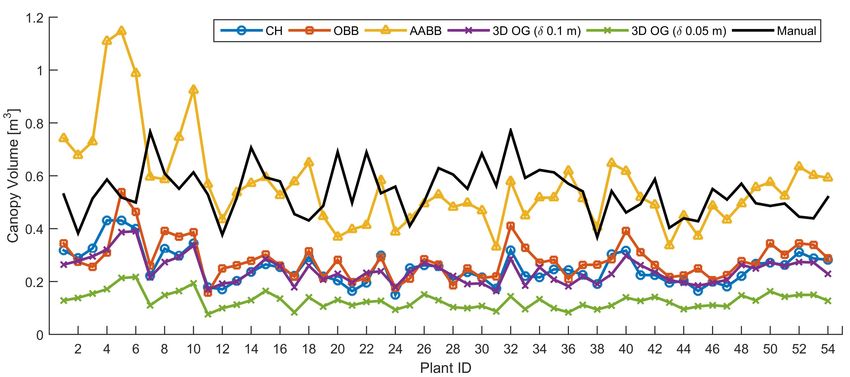
the agronomically relevant traits are best expressed under real environmen-
tal conditions, which are highly heterogeneous and difficult to reproduce. In
particular, perennial crops like grapevines need phenotypic evaluations to be
done directly in the field. Vineyards typically extend over large areas that
contain thousands of single grapevines, each one characterized by a slightly
different phenotype. Due to these reasons, recently, there has been an in-
creasing interest in field-based HTPPs. In this respect, autonomous vehicles
can play a central role towards the automation of data acquisition and pro-
cessing for phenotyping of crop plants in the field, (Emmi and de Santos,
2017; Reina et al., 2017).
In this work, a grapevine phenotyping platform is proposed that uses an
agricultural vehicle equipped with a RGB-D sensor, i.e., a depth sensing
device that works in association with a RGB camera by augmenting the con-
ventional image with distance information in a per-pixel basis. The system
is intended to be used to acquire visual and geometric 3D information to
reconstruct the canopy of the plants for geometric measurements, such as
plant volume estimates, and to detect and count grapevine clusters. Both
measurements are important indicators of growth, health and yield potential
of grapevines (Liu et al., 2013). Specifically, first, different computational
geometry methods for plant modeling and volume estimation using 3D and
color information acquired by the RGB-D sensor are proposed; then, a deep
learning approach using visual images only is developed to segment the scene
into multiple classes and in particular to detect grapevine clusters.
The proposed framework was validated through experimental tests carried
out in a commercial vineyard in Switzerland, with an Intel RealSense R200

                                      3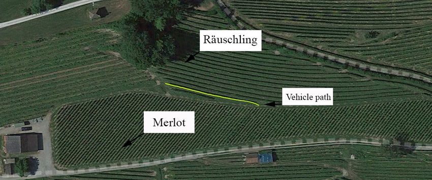
sensor mounted on-board a Niko caterpillar. Compared to traditional man-
ual methods, the main advantage of the proposed approaches is that they
allow for data collection and processing in the field during operations of an
agricultural vehicle, using only a cost-effective 3D sensor. It is shown that,
despite the low quality of the available sensor data, it is possible to extract
useful information about the crop status in a completely automatic and non-
invasive way, thus overcoming time and cost problems related to traditional
man-made measurements.
The rest of the paper is structured as follows. Section 2 reports related work.
The data acquisition system and the proposed algorithms for volume estima-
tion and bunch recognition are described in Section 3. Experimental results
are presented in Section 4. Conclusions are drawn in Section 5.

2. Related Work

   Precision agriculture deals with the application of the right treatment, at
the right place, at the right time (Legg and Stafford, 1998). To this end, the
accurate knowledge of the crop characteristics, or phenotypic data, at sub-
field level is crucial. Conventional approaches to estimate phenotypic traits
are based on human labor using few random samples for visual or destruc-
tive inspection. These methods are time consuming, subjective and prone
to human error, leading to what has been defined the phenotypic bottleneck
(Furbank and Tester, 2011). The lack of phenotypic information limits the
possibility to assess quantitative traits, such as yield, growth and adaption
to abiotic or biotic factors. To overcome this issue, high-throughput phe-
notyping platforms (HTPPs) using different sensor devices, either fixed or

                                      4
mounted on-board mobile vehicles are attracting much interest (Reina et al.,
2016). Research efforts have been especially devoted to build up such plat-
forms under controlled environments (Clark et al., 2011; Hartmann et al.,
2011). Although these systems enable a precise non-invasive plant assess-
ment throughout the plant life cycle under controlled conditions, they do not
take into account the interactions between the plants and the environment.
In contrast, perennial crops like grapevines need to be evaluated directly
in the field. First steps towards a high-throughput phenotyping pipeline in
grapevines have been introduced by Herzog et al. (2014) that developed a
Prototype Image Acquisition System (PIAS) for semi-automated capturing
of geo-referenced images and a semi-automated image analysis tool to phe-
notype berry size. The use of 2D machine vision techniques has been also
proposed in several works to detect grape bunches (Font et al., 2014; Diago
et al., 2012), and to measure berry size or number (Rosell-Polo et al., 2015;
Nuske et al., 2014).
While producing good results, 2D approaches are affected by occlusions. Fur-
thermore, they do not allow to catch important phenotypic parameters such
as 3D plant geometry. To this end, solutions employing stereovision or multi-
view-stereo (MVS) systems have been proposed (Reina and Milella, 2012).
Few of them have been developed in the context of viticulture. Dey et al.
(2012) use a MVS algorithm on images manually collected with a consumer
camera to reconstruct grapevine rows, and developed a Support Vector Ma-
chine (SVM) classifier to segment the point cloud into grape bunches, leaves
and branches. A MVS approach is also developed by ? to reconstruct point
clouds of slightly defoliated grapevines from images acquired by a hand-held

                                     5
camera at daytime. Phenotype traits are then extracted using convex hull,
meshing and computer-aided design (CAD) models. A HTPP for large scale
3D phenotyping of vineyards under field conditions is developed in Rose et al.
(2016). It uses a track-driven vehicle equipped with a five camera system and
a RTK-GPS to reconstruct a textured point cloud of a grapevine row based
on a MVS algorithm. A classification algorithm is then employed to segment
the plant into grape bunches and canopy, and extract phenotypic data such
as quantity of grape bunches, berries and berry diameter.
One big limitation of vision systems is the sensitivity to changing lighting
conditions, which are common in outdoor applications like agriculture. In
such situations, LiDAR sensors have been proved to be much more reli-
able, although they usually need higher investment costs. A LiDAR sensor
mounted on a ground tripod is proposed in Keightley and Bawden (2010)
for 3D volumetric modeling of a grapevine under laboratory conditions. A
ground fixed LiDAR is used in Raumonen et al. (2013) to model the tree
skeleton based on a graph splitting technique. In Auat Cheein et al. (2015),
a LiDAR sensing device carried by a tractor is proposed to scan fruit tree
orchards as the vehicle navigates in the environment and acquire data for
canopy volume estimation through a set of computational geometry meth-
ods. A ground-based LiDAR scanner is used in Arnó et al. (2013) for leaf
area index estimation in vineyards. HTPPs using field phenotyping robots
have been also developed, for applications in maize (Ruckelshausen et al.,
2009), small grain cereals (Busemeyer et al., 2013) and viticulture (Schwarz
et al., 2013; Longo et al., 2010).
As an alternative to vision and LiDAR systems, portable consumer-grade

                                      6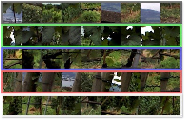
RGB-D sensors, like Microsoft Kinect, have been recently proposed, mostly
in controlled indoor environments such as greenhouses. By including hard-
ware accelerated depth computation over a USB connection, these systems
features a low-cost solution to recover in real-time 3D textured models of
plants (Narvaez et al., 2017). In Paulus et al. (2014) the Kinect and the
David laser scanning system are analyzed and compared under laboratory
conditions to measure the volumetric shape of sugar beet taproots and leaves
and the shape of wheat ears. Depth images from a Kinect are used in Chéné
et al. (2012) to segment and extract features representative of leaves of rose-
bush, yucca and apple plants in an indoor environment. In Chaivivatrakul
et al. (2014), a Kinect is adopted for 3D reconstruction and phenotyping
of corn plants in a controlled greenhouse setting. Depth and RGB cameras
are mounted onboard a mobile platform for fruit detection in apple orchards
(Gongal et al., 2016), whereas structural parameters including size, height,
and volume are obtained for sweet onions and cauliflowers, respectively in
Wang and Li (2014) and Andujar et al. (2016).
Preliminary tests to estimate the grape mass using a Kinect sensor are pre-
sented in Marinello et al. (2017a). An application of the Kinect sensor
for three-dimensional characterization of vine canopy is also presented in
Marinello et al. (2017b), using the sensor statically positioned in the vine-
yard. Although recent developments of Kinect have led to higher robustness
to artificial illumination and sunlight, some filters need to be applied to over-
come the increased noise effects and to reach exploitable results (Rosell-Polo
et al., 2015), therefore the application of this sensor remains mostly limited
to indoor contexts and for close range monitoring (Lachat et al., 2015; Zen-

                                       7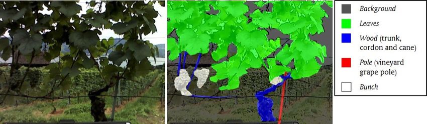
naro et al., 2015).
In 2015, Intel introduced a novel family of highly portable, consumer depth
cameras based on infrared stereoscopy and an active texture projector, which
is similar to the Kinect sensor in scope and cost, but with a different working
principle. The main advantage of this sensor with respect to Kinect is that it
can work in zero lux environment as well as in broad daylight, which makes
it suitable for outdoor conditions. In addition, its output include RGB in-
formation, infrared images and 3D depth data, thus covering a wide range
of information about the scene. Hence, this sensor potentially provides an
affordable and efficient solution for agricultural applications. Previous work
has shown that the RealSense can be successfully used for 3D visual mapping
tasks (Galati et al., 2017).
To the best of our knowledge, the study presented in this paper is the first
application of this kind of RGB-D sensor in the context of in-field grapevine
phenotyping. Mounted on an agricultural tractor, the sensor is able to pro-
vide ground-based 3D information about the canopy volume. At the same
time, using RGB images only it is possible to detect and count grape clusters.
The main contribution of the proposed system is that data acquisition and
processing can be carried out during vehicle operations, in a non-invasive and
completely automatic way, requiring at the same time low investment and
maintenance costs.
Another contribution of the proposed approach regards the use of a deep-
learning based method for grape bunch recognition. In the last few years,
deep learning (LeCun et al., 2015) has become the most promising technique
of the broad field of machine learning for applications in the agricultural

                                      8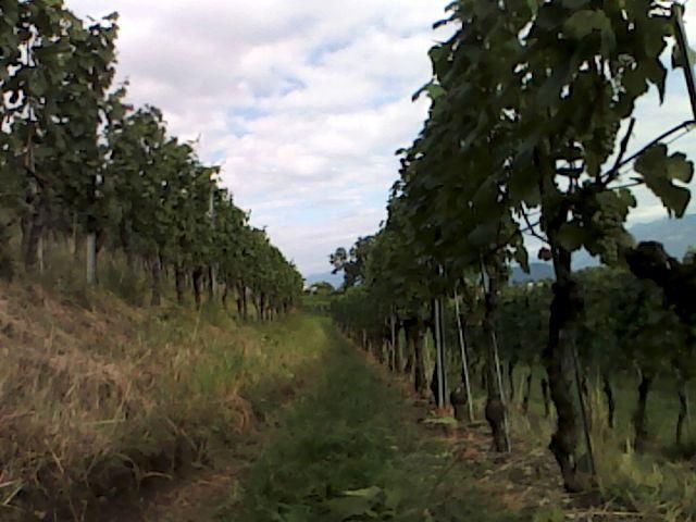
scenario (Kamilaris and Prenafeta-Boldú, 2018). The capacity of deep learn-
ing to classify data and predict behaviors with high flexibility allows its use
in fruit recognition and counting in orchards from visual images (Sa et al.,
2016; Bargoti and Underwood, 2017; Rahnemoonfar and Sheppard, 2017).
In addition, deep-learning-based approaches have demonstrated high capa-
bility in plant identification (Lee et al., 2015; Grinblat et al., 2016), enabling
their use for weed-detection from aerial images (dos Santos Ferreira et al.,
2017). At the same time, several studies have been proposed for image-
based plant disease classification (Ferentinos, 2018; Too et al., 2018). The
improved capabilities of deep learning in comparison with standard machine
learning derive from the higher complexity of the networks, since phenomena
(or corresponding data) under analysis are characterized by hierarchical rep-
resentations. Such representations are computed through the application of
consecutive layers of filters, whose aggregation constitutes the artificial net.
These filters create higher abstractions as data flows ”deeper” in the net.
Preliminary training of the net can automatically determine the best filters,
i.e. the most significant and robust features, to achieve classification.
In this work, a comparative study of four pre-trained convolutional neu-
ral networks (CNNs) designed to achieve the task of grape bunch recogni-
tion is reported. Following the paradigm of transfer learning Yosinski et al.
(2014), the four pre-trained CNNs, namely the AlexNet (Krizhevsky et al.,
2012), the VGG16 and the VGG19 (Simonyan and Zisserman, 2014), and the
GoogLeNet (Szegedy et al., 2015), are tuned by a lower number of samples
of the training set, thus enabling image-based grape cluster detection.

                                        9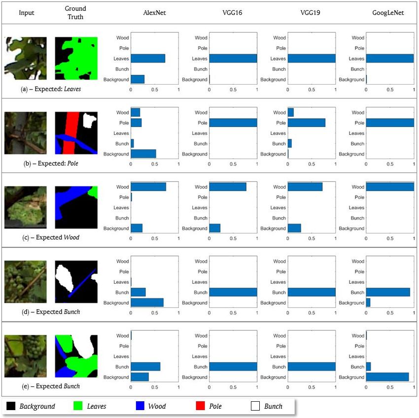
Figure 1: Pipeline of the proposed framework for in-field crop volume estimation and
grape bunch detection.

3. Materials and Methods

   A sensing framework is proposed to automatically estimate the crop vol-
ume and detect grape bunches in vineyards, using a low-cost RGB-D sensor
mounted on-board an agricultural vehicle. The overall processing pipeline
is explained in Figure 1. The sensor provides an infrared (IR) stereo pair
and a RGB image, which are fed to an algorithm for 3D reconstruction of
a grapevine row and canopy segmentation from the trunks and other parts
of the scene. The segmented canopy is successively processed using a set of
computational geometry methods to estimate the volume of the plants. In
addition, color images are used as input to a deep learning-based approach
to recognize grape clusters.
Data for algorithm development and testing were acquired in a commercial
vineyard of a white variety of wine grape, named Räuschling, located in
Switzerland.

                                        10
3.1. Acquisition platform
An Intel RealSense RGB-D R200 imaging system was used. It includes
a left-right stereo pair and a color camera. The stereo pair consists of two
global shutter VGA (640 × 480) CMOS monochrome cameras with a visible
cut filter at approximately 840 nm, with a nominal baseline of 70 mm and a
nominal field of view of 60(H) × 45(V ) × 70(D) deg. They run at 30, 60 or
90 Hz. The color camera is a FullHD (1920 × 1080) Bayer-patterned, rolling
shutter CMOS imager. Although, a global shutter approach may ensure bet-
ter performance, it results in significantly higher cost and complexity. In
addition, during the experimental campaign the CMOS imager proved to be
effective with negligible rolling shutter type artifacts. The stream acquired
by the color camera is time-synchronized with the stereo pair. Its nominal
field of view is of 70(H) × 43(V ) × 77(D) deg and runs at 30Hz at FullHD
and higher frame rate for lower resolutions. The R200 sensor also includes an
infrared texture laser-based (Class 1) projector with a fixed pattern, which
helps improving image matching in texture-less surfaces, which is especially
useful in indoor environments, where homogenous regions are more likely to
occur.
The sensor was mounted on-board a commercial Niko caterpillar (see Figure
2). The camera was mounted first laterally, facing the side of the central-
lower part of the canopy, where most of grape clusters can be typically found.
A forward looking configuration was adopted instead for the task of volume
estimation, due to the relatively limited vertical field of view of the camera
and maximum allowed distance of the vehicle with respect to the row during
the traversal, which did not make possible to frame the entire canopy of the
11Figure 2: Niko caterpillar vehicle used for experimentation equipped with a multi-sensor
suite.
plants when the camera was pointing laterally. Two sample images acquired
using the lateral and forward looking camera configuration are shown in Fig-
ure 3 (a) and (b) respectively.
Images were acquired using the ROS librealsense library. Due to limitations
on the on-board storage capability of the acquisition systems, image resolu-
tion was limited to 640 × 480 for color images with a frame rate of 5 Hz. In
addition, color images were compressed using the compressed image transport
plugin package that enables a JPG compression format.
3.2. Canopy volume estimation
The proposed approach for canopy volume estimation consists of three
main phases:
1. 3D grapevine row reconstruction;
2. grapevine segmentation;
3. plant per plant volume estimation.
12(a) (b)
Figure 3: Sample images acquired by the R200 camera, (a) mounted laterally and (b)
mounted in a forward looking configuration.
3.2.1. 3D grapevine row reconstruction
The first step of data processing consisted in building a color 3D point
cloud representative of the whole grapevine row. The R200 features an on-
board imaging processor, which uses a Census cost function to compare left
and right images, and generate depth information. The algorithm is a fixed
function block and most of its matching parameters are not configurable (Ke-
selman et al., 2017). In particular, it uses a fixed disparity search range of 64
with a minimum disparity of 0, which, at the given resolution, corresponds
to a range of reconstruction distances from about 0.65 m up to infinity. In-
stead, a disparity search range of [8, 40] pixel corresponding to a depth range
of approximately 1.0 to 5.5 m was found to be a good choice for the task
at hand. Therefore, the depth output by the camera was not employed in
this study, and the infrared stereo pair was used as input to a stereo recon-
struction algorithm running on an external computing device. A calibration
13stage was preliminarily performed to align the IR-generated depth map with
the color image, as well as to estimate the sensor position with respect to
the vehicle, based on a calibration procedure using a set of images of a pla-
nar checkerboard1 . Then, for each stereo pair, the reconstruction algorithm
proceeds as follows:
• Disparity map computation: to compute the disparity map, the Semi-
Global Matching (SGM) algorithm is used. This algorithm combines
concepts of local and global stereo methods for accurate, pixel-wise
matching with low runtime (Hirschmuller, 2005). An example of raw
images and corresponding disparity map is shown in Figure 4. In par-
ticular, Figure 4(a)-(b) show the infrared left-right images and Figure
4(c) displays the corresponding color frame. Figure 4(e) shows the dis-
parity map computed by the SGM algorithm in comparison with the
one streamed out by the sensor in Figure 4(d). It can be seen that the
latter provides a sparse reconstruction of the scene, including many
regions not pertaining to the grapevine row of interest (i.e., the one on
the right side of the picture), which could negatively affect the over-
all row reconstruction process. Instead, the disparity search range of
the SGM algorithm was set to better match the region of interest in
the scene. Additional stereo processing parameters, such as block size,
contrast and uniqueness thresholds, were also configured as a trade-off
of accuracy and density.
• 3D point cloud generation: being the stereo pair calibrated both in-
1
http://www.vision.caltech.edu/bouguetj/calib doc/
14trinsically and extrinsically, disparity values can be converted in depth
values and 3D coordinates can be computed in the reference camera
frame for all matched points (?). Only the points for which also color
information is available from the color camera are retained, so as to
obtain a 3D color point cloud. Point coordinates are successively trans-
formed from camera frame to vehicle frame, using the transformation
matrix resulting from the calibration process.
• Point selection: a statistical filter is applied to reduce noise and remove
outlying points. Furthermore, only the points located within a certain
distance from the right side of the vehicle are selected. This allows to
discard most of the points not pertaining to the grapevine row.
Subsequent point clouds are stitched together to produce a 3D map. To
this end, the vehicle displacement between two consecutive frames is esti-
mated using a visual odometry algorithm (Geiger et al., 2011). A box grid
filter approach is then applied for point cloud merging. Specifically, first,
the bounding box of the overlapping region between two subsequent point
clouds is computed. Then, the bounding box is divided into cells of specified
size and points within each cell are merged by averaging their locations and
colours. A grid step of 0.01 m was used as a compromise between accu-
racy and computational load. Points outside the overlapping region remain
untouched.
3.2.2. Grapevine segmentation
In this phase, first, a segmentation algorithm is applied to separate the
canopy from the trunks and other parts of the scene not pertaining to the
15(a) (b) (c)
(d) (e)
Figure 4: (a)-(b) Left-right infrared images and (c) corresponding color image. (d) Dispar-
ity map obtained from the on-board sensor computation. (e) Result of the SGM algorithm
with custom stereo parameters settings.
16canopy, such as the ground. Then, each single plant is detected using a
clustering approach. In order to detect the grapevine canopy, first of all,
green vegetation is identified in the reconstructed scene based on the so-
called Green-Red Vegetation Index (GRVI) (Tucker, 1979). The GRVI is
computed as:
ρgreen − ρred
GRV I = (1)
ρgreen + ρred
where ρgreen/red is the reflectance of visible green/red. In terms of balance
between green and red reflectance, three main spectral reflectance patterns
of ground cover can be identified:
• green vegetation: where ρgreen is higher than ρred ;
• soil (e.g., sand, silt, and dry clay): with ρgreen lower than ρred ;
• water/snow: where ρgreen and ρred are almost the same.
According to Eq. 1, green vegetation, soil, and water/snow have positive,
negative, and near-zero values of GRVI, respectively. It has been shown that
GRV I = 0 can provide a good threshold value to separate green vegetation
from other elements of the scene (Motohka et al., 2010).
An algorithm for segmenting canopy from other parts of the scene was de-
veloped. First, the point cloud was divided into 3D grid cells of specified
side. Then, for each cell the percentage p of points with positive GRVI with
respect to the total number of points, and the average height H above the
ground were computed. Only the cells with p > T hp and H < T hH were la-
beled as belonging to the grapevine canopy. For the given dataset, a value of
T hH of 75 cm and T hp of 70% were found to give good segmentation results.
17Once the points pertaining to the row canopy have been selected, the single
plants must be identified for the successive plant per plant volume estimation
step. To this aim, the point cloud resulting from the canopy segmentation
process was used to feed a K-means algorithm.
3.2.3. Plant per plant volume estimation
Based on the results of the clustering algorithm, different computational
geometry approaches were implemented to model the single plants and per-
form plant per plant volume estimation, as follows:
• 3D occupancy grid (OG): a box grid filter is applied, which divides
the point cloud space into cubes or voxels of size δ. The voxel size
is a design parameter that is typically chosen as a trade-off between
accuracy and performance (Auat Cheein et al., 2015). Points in each
cube are combined into a single output point by averaging their X,Y,Z
coordinates, and their RGB color components. The volume of a plant is
estimated as the sum of the volumes of all voxels belonging to the given
plant foliage. This method is the one that ensures the best fitting of the
reconstructed point cloud. It could lead however to an underestimation
of the real volume in case of few reconstructed points, e.g., due to failure
of the stereo reconstruction algorithm.
• Convex Hull (CH): this method consists in finding the volume of the
smallest convex set that contains the points from the input cloud of a
given plant (Berg et al., 2000). This method does not allow to prop-
erly model the concavity of the object, and could therefore lead to an
overestimation of the volume.
18• Oriented bounding box (OBB): this approach consists in finding the vol-
ume of the minimal bounding box enclosing the point set, (O0 Rourke,
1985). This method could lead to an overestimation of the plant volume
as it is affected by the presence of outliers or long branches.
• Axis-aligned minimum bounding box (AABB): in this case the volume is
defined as the volume of the minimum bounding box (O0 Rourke, 1985)
that the points fit into, subject to the constraint that the edges of the
box are parallel to the (Cartesian) coordinate axes. As the OBB and
CH approach, the AABB method can lead to an overestimation of the
volume as it does not model properly plant voids and is affected by
outliers or long branches.
The results obtained by each of these automatic methods were compared to
the measurements obtained manually in the field at the time of the exper-
imental test. In the manual procedure, the plant width is assumed to be
constant and equal to the average distance between two consecutive plants
(i.e., 0.9 m), whereas plant depth and height are measured with a tape; then,
the volume is recovered as the product of width, depth, and height.
3.3. Grape cluster recognition
Grape cluster recognition is performed by exploiting four convolutional
neural networks (CNN), namely the pre-trained AlexNet (Krizhevsky et al.,
2012), VGG16 and VGG19 (Simonyan and Zisserman, 2014), and GoogLeNet
Szegedy et al. (2015). All networks allow for labeling input RGB images
among 1000 different classes of objects, but with different architectures:
19• AlexNet: A feed-forward sequence of 5 convolutional layers and 3 fully-
connected layers. The first convolutional layer has a size of 11x11,
whereas the remaining have filter size of 3 × 3;
• VGG16: A feed-forward sequence of 13 convolutional layers and 3 fully-
connected layers. All convolutional layers have filter sizes of 3 × 3;
• VGG19: A feed-forward sequence of 16 convolutional layers and 3 fully-
connected layers. All convolutional layers have filter sizes of 3 × 3;
• GoogLeNet: A feed-forward sequence of 3 convolutional layers of 7 × 7,
1×1 and 3×3 filter sizes, 9 inception layers, each one made of 4 parallel
blocks (without convolution and with 1 × 1, 3 × 3, 5 × 5 convolutional
layers), and a single fully-connected layer at the end of the chain.
In all cases, the weights of the networks are determined during a training
phase performed on a dataset of 1.2 million images.
Although these networks are devoted to solve the task of image labelling
among generic classes, they can be tuned by keeping the first layers of the
net and by rearranging the last fully-connected layer in order to solve more
specific classifications. Under this condition, the whole architecture is almost
completely initialized and, consequently, its parameters can be easily tuned
by a smaller, but much more focused and target-oriented dataset. In particu-
lar, here, the task of recognition is performed to classify input image patches,
having size of the input layer of the CNNs (227 × 227 for the AlexNet and
224 × 224 for the others), among 5 different classes of interest:
• grapevine bunches;
20Figure 5: Example of an input image and the corresponding manual segmentation in five
classes of interest: white, red, blue, green and black refer to Bunch, Pole, Wood, Leaves
and Background, respectively.
• vineyard grape poles;
• grapevine trunks, cordons and canes (wood);
• leaves;
• background.
An example of segments extracted from a labelled input image is reported
in Figure 5. It is worth noticing that the background class includes regions
of pixels which are actually very similar to those of the other classes. For
instance, leaves of far plants are almost similar to grape bunches of the fore-
ground. The network shall discriminate between similarities to reduce false
positives or false negatives.
Given the number of output classes, the starting CNNs have been changed
by substituting the last fully-connected layer with another one made of only
5 neurons, one for each expected output class. This layer is then followed by
a softmax layer to compute classification scores. This fully-connected layer
is not initialized and its weights have to be selected from scratch. Therefore,
21training the transfer nets requires different learning rates to keep the features
from the early layers of the pre-trained networks. Specifically, the learning
rate of the fully-connected layer is 20 times higher than the one of the trans-
ferred layer weights: this choice speeds up learning in the new final layer.
Training options are finally selected to run the learning phase on a single
GPU (nVidia Quadro K5200). For instance, input data is divided in mini-
batches, whose size is defined accordingly with the number of unknowns of
the CNNs and the capability of the GPU (see Table 2 for details). At the end
of each iteration the error gradient is estimated and the network parameters
are updated in accordance with the principles of stochastic gradient descent
with momentum (SGDM) optimization (Sutskever et al., 2013). Training is
performed using two different datasets: the training and the validation sets.
The former is used to estimate the network parameters by backpropagating
the errors; the latter is proposed to the net at the last iteration of each epoch,
in order to compute the validation accuracy and validation loss in feed for-
ward for the current network parameters. If the validation loss does not go
down for 10 consecutive epochs, the training of the network ends.
3.3.1. Dataset generation
As previously reported, each CNN is designed to receive input images of
N × N size (N = 227 for AlexNet and N = 224 for the other CNNs) and to
output labels in a set of 5 possible classes. However, color frames of 640×480
pixels were available from the R200 sensor. The whole set of visual images
acquired during experiments and manually segmented in the 5 classes of in-
terest is made of 85 images. This set is randomly divided in two datasets
with a proportion of 0.7-0.3. The first set is used for training purposes and is
22further separated in the training and validation sets. The second set is made
of test images, which will be proposed to the network after its training, in
order to compute quality metrics. These images are not known to the net-
work which will proceed to labelling.
The target of image analysis is the detection and localization (segmentation)
of grape bunches within the input images. This problem can be solved by
moving a square window, whose size is large enough to frame bunches, and by
processing each resulting patch. Then, depending on the classification score,
grape clusters can be detected and thus localized within the images. Specif-
ically, grape bunches have sizes which depend on the camera field-of-view
and the plant distance. Under the current working conditions, bunches can
be framed in windows whose sizes do not exceed 80×80 pixels. Accordingly,
the proposed algorithm processes input images by moving a 80-by-80-window
at discrete steps, in order to extract image patches. This process of patch
extraction is speeded up by means of a pre-determined look-up table, filled
by the indices, i.e. memory positions, of each entry of the expected patches.
These windowed images will then feed the network in both training and test
phases. Before feeding the network, patches are upscaled using bicubic in-
terpolation to the target size of N×N, in order to match the input layer of
the corresponding CNNs. It is worth noticing that bicubic interpolation can
add artifacts to input images, such as edge rounding, which can down the
accuracy of classification results (Dodge and Karam, 2016). However, all
images of both training and test datasets are upscaled to the same patch
size and, thus, upscaling distortions equivalently affect both datasets. As a
consequence, the networks are trained by distorted images and tune their
23Figure 6: Flow chart for labeling of input training patches among the five output classes.
weights to process test images with the same distortions of the training one.
As a result, classification will not be altered by upscaling distortions, since
the networks are already trained to manage them. Examples for training the
network are created by labelling each image patch of the training and valida-
tion sets depending on the number of pixel belonging to a specific class. In
this case, the choice is made by a weighted summation pixel labels, in order
to give more significance to pixels of bunch, pole and wood classes. The
simple flow chart for patch labeling is reported in Figure 6. For instance, if
24Figure 7: Sample patches used to fine-tune the CNNs. Black, green, blue, red and white
frames refer to background, leaves, wood, pole and bunch classes, respectively.
the summation of pixels of the bunch class goes beyond 20% of the whole
number of pixels of the input patch (more than 1280 over 6400 pixels, before
upscaling), the example trains the network as bunch. Moving the window
and counting the pixels of the ground truth generates 44400, 5295, 3260,
7915 and 81687 patches of the classes leaves, bunch, wood, pole and back-
ground, respectively. A subset of patches of the training and validation sets
is presented in Figure 7.
4. Results and Discussion
Field tests were performed in a commercial vineyard in Switzerland. A
picture showing a Google Earth view of the testing environment is reported
in Figure 8. The vehicle trajectory estimated by an on-board RTK GPS
system is overlaid on the map in Figure 8. Data were acquired by driving
the vehicle from left to right at an average speed of 1.5 m/s. 640×480 stereo
25Figure 8: Google Earth view of the testing environment in a commercial vineyard in
Switzerland. It comprises two types of grapes, namely Räuschling and Merlot. The yellow
line denotes the vehicle path as estimated by an on-board RTK GPS system during the
experiment.
frames and corresponding color images were captured at a frame rate of 5
Hz. The row to the right side in direction of travel, including 55 plants, is
considered in this study. Note that the fifth plant in the direction of motion
was judged to be dead by visual inspection and was not considered in this
work, resulting in a total of 54 surveyed plants.
4.1. Canopy volume estimation
The output of the 3D reconstruction method for the grapevine row un-
der analysis is reported in Figure 9. It comprises about 1.3M points. The
corresponding GRVI map is shown in Figure 10 where lighter green denotes
higher values of GRVI. The result of the segmentation algorithm using GRVI
and 3D information is shown in Figure 11: points displayed in green pertain
to the plant foliage, whereas black points are classified as non-leaf points and
26Figure 9: 3D reconstruction of the grapevine row under inspection. It includes 55 plants
spanning along a total length of approximately 50 m. Plants are located at approximately
0.90 m apart with respect to each other.
Figure 10: GRVI map: green points correspond to green vegetation; blue points correspond
to non-vegetated regions. Lighter green corresponds to higher GRVI.
are not considered for the subsequent volume estimation procedure.
Points classified as pertaining to plant foliage were further processed by
k-means clustering. The number of clusters was fixed at 54. Centroids were
initialized knowing that plants are approximately located at an average dis-
tance of 0.90 m with respect to each other. Figure 12 shows the result of the
clustering process. Each cluster is represented by a different color. Non-leaf
points are also displayed in their original RGB color. For each cluster, the
Figure 11: Segmentation results: green points pertain to foliage, whereas black points
belong to other parts of the scene.
27Figure 12: Result of the clustering process. Single plants are represented by a different
color, for a total of 54 plants. Non-leaf points are displayed in their original RGB color.
volume was estimated using the four methods described in Section 3.2.3, and
was compared with the manual measurements.
Figure 13 shows, as an example, the result of plant modeling using the dif-
ferent methods for five individuals. Estimated volumes for all individuals
are shown in Figure 14. The corresponding descriptive statistics in terms of
mean, standard deviation, minimum and maximum measure are reported in
Table 1. These results show that methods not taking into account concavities
and voids such as CH, OBB, and AABB, result in higher estimates, with the
AABB method most approaching the manual measurements with an average
discrepancy of about 5%. A significantly smaller volume is obtained using
the 3D-OG approach with a voxel grid size δ = 0.05 m, due to disconnected
structures and voids in the model. This effect is mitigated when increasing
the grid size up to 0.1 m, with results getting closer to the CH and OBB
methods.
As a final remark, it should be noted that the availability of the 3D point
cloud pertaining to each single plant makes it possible to extract other geo-
metric traits of interest. As an example, Figure 15 shows the estimation of
the canopy height, obtained as the vertical extension of the minimum bound-
ing box for the same vineyard row. Individual plants are coloured based on
the estimated canopy height according to the color bar shown at the bottom
28(a) (b)
(c) (d)
(e)
Figure 13: Result of plant modeling for plants from 10th to 14th using 3D occupancy grid
with δ = 0.05 m (a) and δ = 0.1 m (b), convex hull (c), oriented bounding box (d) and
axis-aligned minimum bounding box (e).
29Figure 14: Plant volume estimates obtained using different automatic methods compared
with a manual approach.
Table 1: Descriptive statistics of canopy volume (m3 ) by different methods.
Mean St. Dev. Min. Max.
METHOD (m3 ) (m3 ) (m3 ) (m3 )
OG (δ = 0.05m) 0.127 0.031 0.076 0.217
OG (δ = 0.1m) 0.241 0.050 0.164 0.390
CH 0.252 0.064 0.150 0.431
OBB 0.281 0.072 0.158 0.538
AABB 0.564 0.169 0.331 1.147
Manual 0.539 0.091 0.368 0.771
30Figure 15: Canopy height estimated as the vertical extension of the minimum bounding
box of individual plants. The color of each plant reflects the canopy height according to
the color bar shown at the bottom of the figure.
of Figure 15. Non-leaf points are also displayed in their original RGB color.
The average canopy height resulted in 1.25 m with a standard deviation of
0.12 m.
4.2. Grape cluster detection
The pre-trained CNNs have been fine-tuned to perform the classification
among the five classes of interest, through proper training. Then, they have
been used to label test patches and to compare final scores in prediction
tasks. This section describes the evaluation metrics for the assessment of
results, the training phase on labelled images and the final tests on unknown
data.
4.2.1. Evaluation metrics
As already shown in the previous sections, the CNNs receive square im-
age patches of N×N pixels (N = 227 for AlexNet and N = 224 for VGG16,
VGG19 and GoogLeNet). Each input patch of both training and test sets
has a corresponding label, among the five target classes, determined by man-
ual segmentation of the dataset. Accordingly, it is possible to define some
metrics which will be helpful for the final evaluation of the net performance.
31With reference to multiclass recognition, for each class c, the final results of
training will be presented by counting true and false predictions of class c
against the others. It leads to true positives (T Pc ) and negatives (T Nc ), and
false positives (F Pc ) and negatives (F Nc ). These values are further processed
to determine accuracy (ACCc ), balanced accuracy (BACCc ), precision (Pc ),
recall (Rc ), and true negative rate (T N Rc ), which have the following formu-
lations:
T Pc + T Nc
ACCc = (2)
T Pc + F Pc + T Nc + F Nc
T Pc T Nc
T Pc +F Nc
+ T Nc +F Pc
BACCc = (3)
2
T Pc
Pc = (4)
T Pc + F P c
T Pc
Rc = (5)
T Pc + F N c
T Nc
T N Rc = (6)
T Nc + F Pc
Specifically, ACCc estimates the ratio of correct predictions over the whole
occurrences, while BACCc also weights standard accuracy by the number of
occurrences of the cth class. As a consequence, BACCc overcomes misleading
interpretations of results due to the heavy unbalancing of occurrences of the
cth class in comparison to the other classes. Pc shows whether all detections
of the cth class are true, whereas Rc states the ability of the CNN to label
a patch of the cth class, recognizing it against the others. Finally, T N Rc
inverts the meaning of Rc , i.e. it defines how the CNN is capable of not
assigning the label c to patches of the other classes. Metrics in Eq. 2 to
6 refer to pixel-by-pixel, i.e. per-patch, evaluations. Specifically, they can
32be effectively used for stating whether the architecture of the CNNs and
the input examples are suitable to allow the classification of the training
patches (training assessment). On the other hand, the result of tests will
be evaluated to measure the actual capability of the CNN to detect grape
clusters in 25 test images, knowing the number of bunches in each image,
instead of evaluating the results of per-pixel segmentation. In this case,
accuracy (ACCGC ), precision (PGC ) and recall (RGC ) are redefined as:
TGC
ACCGC = (7)
GC
TGC
PGC = (8)
TGC + FGC
TGC
RGC = (9)
TGC + NGC
where GC is the total number of grape clusters, TGC is the number of true
detections, FGC is the number of wrong detections and NGC is the number
of missed detections of grape clusters.
4.2.2. Training of the CNNs
The training phase is performed by feeding the CNNs with 142000 sam-
ple patches, which are divided into training and validation sets in propor-
tion 0.75-0.25. As previously stated, two different learning rates have been
selected for the first layers, transferred from the CNNs, and for the last
fully-connected layers. Specifically, the learning rate for the first layers is
set to 10−4 , whereas the last fully-connected layer, responsible for the final
classification in the five classes of interest, is trained with a learning rate
of 2 · 10−3 . The SGDM optimization is reached with a momentum of 0.9.
These parameters produce the results in Table 2, which reports the required
33Table 2: Number of epochs and time requirements for the learning phase of the four
proposed CNNs.
Mini-batch Number of Total training Training time
CNN size epochs time per epoch
(no. of samples) (h) (min)
AlexNet 210 17 4.0 14.1
VGG16 35 15 57.5 230
VGG19 10 11 49.1 268
GoogLeNet 21 22 20.2 55.1
number of epochs for reaching the convergence of the learning phase, and the
corresponding time consumption (total and per-epoch), valid for the corre-
sponding mini-batch size, whose dimension is defined to work at the memory
limit of the GPU used for experiments.
The analysis of Table 2 shows that the AlexNet, which is significantly
less complex than any other CNN of this comparison, can be trained in 4
hours. On the contrary, the other CNNs require more than about 20 hours
(see the GoogLeNet) to complete the learning phase. Quantitative results on
the network performance are in Table 3, which shows the evaluation metrics
in Eq. 2 to 6, computed by joining both the training and validation sets.
The inspection of the results in Table 3 reveals that the balanced accuracy
is always higher than 94.13% for all the CNNs (see the balanced accuracy of
class wood of the AlexNet). With respect to the bunch class, the training
phase of every proposed CNN ends with satisfying values of BACCbunch ,
Pbunch and Rbunch . Among these values, precision is comparable, but always
34Table 3: Results of training. These metrics are computed based on Eq. 2 to 6 for the
whole training set, made of both training and validation patches.
CNN Class ACC c BACC c Pc Rc T N Rc
Background 0.96054 0.96176 0.97714 0.95344 0.97007
Leaves 0.97264 0.9726 0.94160 0.97248 0.97272
AlexNet Wood 0.99508 0.94131 0.89819 0.88497 0.99765
Pole 0.99527 0.98109 0.95048 0.96513 0.99704
Bunch 0.99347 0.97482 0.87974 0.95467 0.99497
Background 0.99364 0.99362 0.99356 0.98586 0.99368
Leaves 0.99888 0.99291 0.98646 0.98368 0.99937
VGG16 Wood 0.99882 0.98907 0.97882 0.97261 0.99932
Pole 0.99866 0.99744 0.99607 0.98002 0.99881
Bunch 0.99080 0.99113 0.98892 0.99507 0.99335
Background 0.9919 0.9897 0.98399 0.98957 0.9954
Leaves 0.99623 0.99642 0.99661 0.91078 0.99622
VGG19 Wood 0.99795 0.98169 0.96461 0.95136 0.99878
Pole 0.99863 0.99426 0.98934 0.98596 0.99918
Bunch 0.98605 0.98608 0.98589 0.98985 0.98626
Background 0.98916 0.99067 0.99461 0.9708 0.98674
Leaves 0.99732 0.96642 0.93303 0.99479 0.99981
GoogLeNet Wood 0.9966 0.99189 0.98695 0.88571 0.99684
Pole 0.99873 0.99491 0.99061 0.98648 0.99921
Bunch 0.98370 0.98460 0.97873 0.99289 0.99047
35lower than recall. It suggests that bunches will be detected with high rates,
but among these detections several false positives could arise. For this reason,
further processing, such as morphological filters on per-pixel segmentation,
will be required to improve results in grape cluster detection.
4.2.3. Test of the CNN
A test set of 25 images was used for evaluation purposes. Following the
same approach developed for the training set, images are separated in smaller
square patches, whose size is as large as the expected dimension of grape clus-
ters (80×80 pixels). Then, these patches are upscaled in order to meet the
requirements of the input layer of the transferred CNNs. Each patch is finally
labelled by the class of the highest relevance.
Test patches are used to feed the CNN, which returns 5 classification scores
about the image label. As an example, Figure 16 shows the results of patch
labelling in ambiguous cases, where the same patch has objects of differ-
ent classes. As can be seen, each object (i.e., bunches, leaves, wood pieces
and poles) contributes to increase the score of the corresponding class. In
addition, as effect of the strategy adopted to label training patches, i.e. la-
belling the patches giving more weight to bunches, wood pieces and poles
with respect to leaves and background, small parts of such objects have
more influence to the final estimation of class probability. With reference to
Figure 16(d) and (e), few grapes surrounded by many leaves and/or large
background areas will anyway produce the rise of the probability (score) of
the bunch class.
This aspect is emphasized for the VGG16 and VGG19, which label the
bunch patches with the highest probability (equal to 1), although patches in
36Figure 16: Results of tests on sample patches. Bar plots report the probabilities (classifica-
tion scores) of image labels for the corresponding patches, by varying the CNN (AlexNet,
VGG16, VGG19 and GoogLeNet). Pixel-by-pixel ground truths are reported for each pixel
of the patches. Black, green, blue, red and white refer to regions of background, leaves,
wood, pole and bunch, respectively. Patch labels are: (a) leaves, (b) pole, (c) wood and
(d)-(e) bunch.
37Table 4: Time elapsed for the classification of 12314 patches extracted from a single input
image.
CNN Time (s)
AlexNet 27.18
VGG16 417.56
VGG19 521.84
GoogLeNet 331.40
16(d) and (e) have background, leaves and wood regions of extended area. On
the contrary, the AlexNet and the GoogLeNet can fail in labeling bunches,
as clearly shown by the inspection of corresponding probability values in Fig-
ure 16(d) and (e), respectively. In both cases background scores are higher
than those of the bunch class, expected for the two inputs. Performance can
be compared also in terms of time requirements for the complete classifica-
tion of an input image. These requirements are reported in Table 4, which
shows the time elapsed for the classification of 12314 patches, taken from a
single frame. Time requirements follow the same behavior of the training
phase. Specifically, the VGG19 takes more time with respect to the others,
whereas the AlexNet, which has the simplest architecture, is the fastest CNN
in labeling the whole image. However, this performance, which is obtained
without implementing dedicated hardware, does not allow the online cluster
recognition. As already discussed, each patch is taken from the input image
at specific positions. Its processing produces 5 classification scores.
At each position of the window, these scores can be rearranged to create
5 probability images. Since image analysis is aimed at the detection of grape
38clusters and its coarse segmentation through a bounding box, the probabil-
ity map of the bunch class has to be further processed. Specifically, the
probability maps of class bunch obtained by the classification of the 25 test
images are converted to binary images, based on a threshold, whose level is
fixed to 0.85. As a consequence, all bunch detections performed with scores
higher than 85% are grouped in connected components. These regions are
also processed by simple morphological filters: a morphological closing (di-
lation followed by erosion) on the binary image is performed using a 5 × 5
structural element of circular shape. Finally, the smallest rectangles enclos-
ing the resulting connected components of the binary images determine the
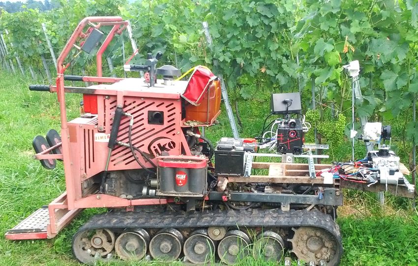
bounding boxes of the detected grape clusters. Three representative images,
output of each CNN, are presented in Figure 17, together with the bounding
boxes (red rectangles) enclosing the detected grape clusters.
Bounding boxes in Figure 17 well include grape clusters, although their
guess suffers from the overestimation of the extension of grape clusters. It is
due to the use of the moving window, since patches with grape cluster placed
at their edges are entirely labeled as bunches. In addition, this overestimation
of bunch sizes also results from the specific choice of the threshold level (0.85
in these experiments). This value has been set to obtain a good balance
between overestimation of grape regions, missed detections (yellow rectangles
in Figure 17), and false positives (cyan circles of Figure 17). For instance, if
the threshold is increased, overestimation and false positives can vanish, but
at the same time further missed detections can arise. With this setting of the
threshold value, only few small grape clusters are not detected as effect of
the low quality of the input image in terms of low resolution and significant
39Figure 17: Sample images with bounding boxes (red rectangles) enclosing the detected
grape clusters. The dashed yellow rectangles locate missed detections of grape cluster,
whereas the cyan circles enclose false detections.
40Table 5: Results of tests on 25 input images, computed accordingly with metrics from Eq.
7 to 9.
FGC /GC NGC /GC PGC RGC AccGC
CNN (%) (%) (%) (%) (%)
AlexNet 12.50 14.30 87.03 85.45 81.03
VGG16 1.90 17.30 98.0 84.48 83.05
VGG19 12.30 10.70 87.09 88.52 91.52
GoogLeNet 2.10 29.16 97.91 77.04 79.66
motion blur. At the same time only small regions of actual ambiguity are
marked as bunches. As an example, the cyan circles of Figure 17 resulting
from the VGG16 and the GoogLeNet are the only false detections obtained
by running the tests on the whole dataset. Quantitative results in terms of
metrics from Eq. 7 to 9 are finally reported in Table 5 for each proposed
CNN.
Results in Table 5 demonstrate that all CNNs can effectively count fruits
regardless the low quality of the input color images. A deeper insight shows
that the VGG19 returns the best accuracy (91.52%) and recall (88.52%) with
respect to the other CNNs, although its precision (87.09%) is worse than
the ones provided by the GoogLeNet (97.91%) and the VGG16 (98.0%).
In particular, the latter CNN can significantly reduce the number of false
predictions to values less than 2% (see the cyan circles of Figure 17). This
means that all recognitions of grape clusters effectively refer to actual fruits.
At the same time the VGG16 produce lower false negatives, i.e. missed
recognitions, than the GoogLeNet, suggesting that it is more sensitive to
the presence of grape clusters with respect to the GoogLeNet. However, the
41AlexNet shows balanced results in terms of precision and recall, which are
almost comparable. Although results from the AlexNet are not the best of
this comparison, it can be preferable because of its lower requirements in
terms of processing time.
5. Conclusions
This paper proposed an in-field high throughput grapevine phenotyping
platform using an Intel RealSense R200 depth camera mounted on-board an
agricultural vehicle. The consumer-grade sensor can be a rich source of infor-
mation from which one can infer important characteristics of the grapevine
during vehicle operations. Two problems were addressed: canopy volume
estimation and grape bunch detection.
Different modeling approaches were evaluated for plant per plant volume es-
timation starting from a 3D point cloud of a grapevine row and they were
compared with the results of a manual measurement procedure. It was shown
that depending on the adopted modeling approach different results can be
obtained. That indicates the necessity of establishing new standards and
procedures. Four deep learning frameworks were also implemented to seg-
ment visual images acquired by the RGB-D sensor into multiple classes and
recognize grape bunches. Despite the low quality of the input images, all
methods were able to correctly detect fruits, with a maximum value of ac-
curacy of 91.52%, obtained by the VGG19. Overall, it was shown that the
proposed framework built upon sensory data acquired by the Intel RealSense
R200 is effective in measuring important characteristics of grapevine in the
field in a non-invasive and automatic way.
42Future work
Both perception methods discussed in the paper use a consumer-grade
camera (worth a few hundred Euros) as the only sensory input. This choice
proved to be a good trade-off between performance and cost-effectiveness.
An obvious improvement would be the adoption of higher-end depth cam-
eras available on the market. A new model of RealSense (D435 Camera)
was just delivered by Intel featuring improved resolution and outdoor perfor-
mance. Another common issue was the large vibrations experienced by the
camera during motion that was induced by the on-board combustion engine
and the terrain irregularity. This calls for a specific study to model the ve-
hicle response and compensate/correct for this disturbance source. The first
method for automatic volume estimation comprises three main stages: 3D
grapevine row reconstruction, canopy segmentation, and single plant volume
estimation. Each stage may be refined improving the overall performance.
For example, the 3D reconstruction of the entire row strongly depends on
the pose estimation of the operating vehicle. In the proposed embodiment,
the robot localization system uses only visual information. However, visual
odometry typically suffer from drift or accumulation errors, especially for
long range and long duration tasks. Therefore, the integration of comple-
mentary sensor types, including moderate-cost GPS and IMU (e.g., (Ojeda
et al., 2006)), may significantly enhance this stage. In addition, the re-
liance on simultaneous localization and mapping (SLAM) approaches may
be certainly beneficial and it would allow continuous estimation between
successive crop rows mitigating the difficulties connected with the 180-deg
steering stage at the end of each row. The canopy segmentation step was
43You can also read