Influence of the Atlantic meridional overturning circulation on the U.S. extreme cold weather
←
→
Page content transcription
If your browser does not render page correctly, please read the page content below
ARTICLE
                  https://doi.org/10.1038/s43247-021-00290-9              OPEN

                  Influence of the Atlantic meridional overturning
                  circulation on the U.S. extreme cold weather
                  Jianjun Yin        1✉   & Ming Zhao2

                  Due to its large northward heat transport, the Atlantic meridional overturning circulation
                  influences both weather and climate at the mid-latitude Northern Hemisphere. Here we use a
                  state-of-the-art global weather/climate modeling system with high resolution (GFDL
                  CM4C192) to quantify this influence focusing on the U.S. extreme cold weather during
                  winter. We perform a control simulation and the water-hosing experiment to obtain two
1234567890():,;

                  climate states with and without a vigorous Atlantic meridional overturning circulation. We
                  find that in the control simulation with an overturning circulation, the U.S. east of the Rockies
                  is a region characterized by intense north-south heat exchange in the atmosphere during
                  winter. Without the northward heat transport by the overturning circulation in the hosing
                  experiment, this channel of atmospheric heat exchange becomes even more active through
                  the Bjerknes compensation mechanism. Over the U.S., extreme cold weather intensifies
                  disproportionately compared with the mean climate response after the shutdown of the
                  overturning circulation. Our results suggest that an active overturning circulation in the
                  present-day climate likely makes the U.S. winter less harsh and extreme.

                  1 Department   of Geosciences, University of Arizona, Tucson, USA. 2 NOAA/GFDL, Princeton, USA. ✉email: yin@arizona.edu

                  COMMUNICATIONS EARTH & ENVIRONMENT | (2021)2:218 | https://doi.org/10.1038/s43247-021-00290-9 | www.nature.com/commsenv   1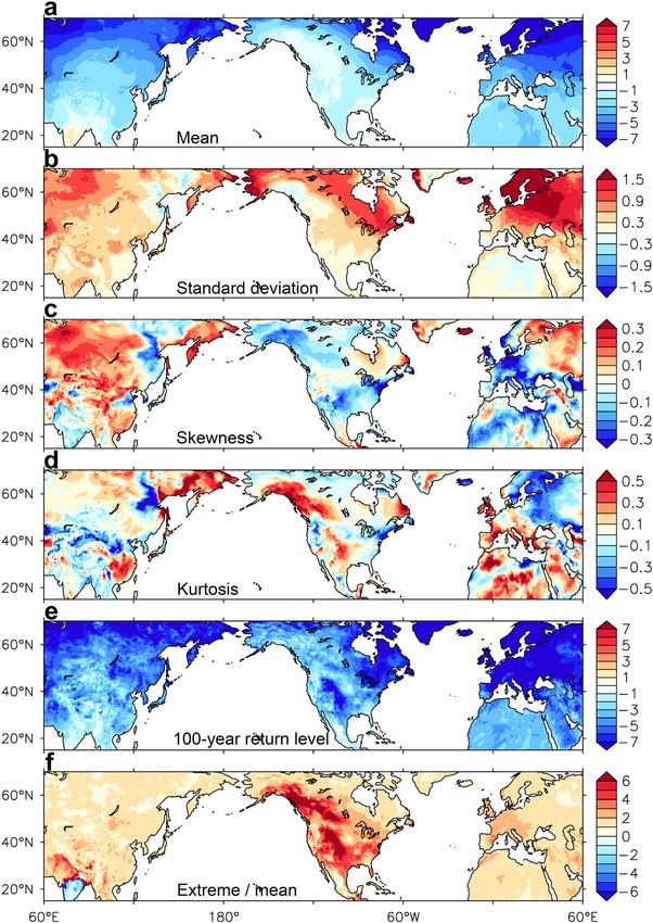
ARTICLE                                             COMMUNICATIONS EARTH & ENVIRONMENT | https://doi.org/10.1038/s43247-021-00290-9

T
        he important role of the Atlantic Meridional Overturning            CM4C192, the atmosphere and ocean work together to transport
        Circulation (AMOC) in the climate system has been exten-            up to 5.7 Petawatts (PW, or 1015 Watts) annual heat poleward to
        sively studied1–12. Without an AMOC and associated                  compensate the differential solar heating between the low and
northward heat transport, northern and western Europe could be              high latitudes27–29 (Fig. 1a, b and Supplementary Fig. 2). In the
much colder1,2,5,6,9, the Arctic sea ice could expand1, the Inter-          Northern Hemisphere, the maximum total transport occurs at
Tropical Convergence Zone (ITCZ) could shift southward3,5,9, and            about 40°N. At mid-latitudes, the atmosphere is highly efficient at
sea level along the East Coast of North America could be higher12.          mixing different temperatures and transporting heat poleward
Compared with these changes in the mean climate, the impact of              through fast-moving turbulent weather systems, especially during
AMOC on extreme weather has not been investigated systematically            winter. For the annual mean, the oceanic transport of about 0.8
and sufficiently thus far. One reason is that previous generations of        PW at 40°N, largely due to AMOC16,30,31, is by far smaller than
global climate model were particularly designed for studies on large-       its atmospheric counterpart of 4.8 PW, but nonetheless represents
scale, long-term climate, rather than on daily weather at the local         an enormous amount of heat in global energy balance (Fig. 1). It
scale, which requires high resolution, frequent data output, regional       should be noted that CM4C192 likely underestimates the
focus, and so on. Nonetheless, several recent studies have shown            northward heat transport in the Atlantic. The simulated max-
that a slowdown of AMOC could contribute to summer heatwaves                imum transport of about 1 PW at 26°N is lower than the recent
over Europe13,14, flooding and droughts15, stronger and more active          observational estimate of about 1.3 PW16,31 (Fig. 1c).
Atlantic hurricanes16,17 and extratropical storms18.                           We consider the atmosphere north of 40°N as a whole
   During the past decade, the Geophysical Fluid Dynamics                   (“northern atmosphere”) and perform a detailed heat budget
Laboratory (GFDL) of NOAA has been working towards a unified                 analysis for December, January, and February (DJF). During
and seamless modeling system suitable for studying both weather and         boreal winter of the control, the northern atmosphere loses 13.3
climate, as well as their complex interactions under the same               PW heat at the top of the atmosphere (TOA) but gains 6.1 PW
umbrella. The recent progress in model development and the rapid            from the surface (Fig. 1a). The heat deficit of 7.2 PW is
growth of supercomputer power have provided better tools to tackle          compensated by the atmospheric heat transport across 40°N
important weather-climate issues. Here, we use the high resolution          mainly associated with mid-latitude weather processes especially
version (C192) of the global coupled modeling system, GFDL                  baroclinic transient eddies. Without an AMOC and its northward
CM419–23 (see the “Methods” section), to investigate the influence of        heat transport in the hosing experiment (Fig. 1c), the TOA and
AMOC on the U.S. extreme cold weather during winter. As low-                surface heat fluxes reduce by 0.6 PW and 1.1 PW, respectively
frequency high-impact events, extreme cold snaps could be disastrous        (Fig. 1a). To compensate the increased heat deficit due to these
(https://www.ncdc.noaa.gov/billions/), particularly for the U.S.            changes, the atmosphere must transport about 0.5 PW more heat
southern states with typical mild temperatures during winter24,25.          northward across 40°N. This “Bjerknes compensation”
                                                                            mechanism32–36 works to stabilize the mean temperature and
                                                                            maintain the energy balance of the northern atmosphere in a
Results
                                                                            climate without AMOC.
Control simulation and water-hosing experiment with GFDL
                                                                               The enhanced atmospheric heat transport during winter is
CM4C192. Under the 1950 radiative forcing, a long, centennial
                                                                            achieved through more active weather processes at mid-
timescale control simulation has been carried out with CM4C192
                                                                            latitudes33. In the control, intense north–south atmospheric heat
as part of the GFDL’s participation in the High Resolution Model
                                                                            exchanges occur over a broad region at 40°N. At 850 hPa, large
Intercomparison Project26. Due to the refined resolution for both
                                                                            atmospheric eddy temperature fluxes27 (v′T′; see “Methods”
the atmosphere (0.5°) and ocean (0.25°), synoptic-scale phe-
                                                                            section) are found over the eastern North America and western
nomena are better simulated by CM4C192, including hurricanes
                                                                            North Atlantic, East Asia, and the North Pacific, as well as over
and severe winter storms, atmospheric rivers and blocking, ocean
                                                                            Europe and Middle East (Fig. 2a). These regions coincide with the
eddies and jets, storm surge and coastal flooding, etc12,19–21,23. In
                                                                            mid-latitude storm track where extratropical cyclones and anti-
addition, the simulated AMOC has a mean strength of about
                                                                            cyclones continuously develop and propagate, thereby efficiently
18 Sv (1 Sv = 106 m3 s−1) at 26°N, compared well with
                                                                            mixing warm and cold air masses. In particular, the U.S. east of
observations19,23 (Supplementary Fig. 1a).
                                                                            the Rocky Mountains37 sees some of the highest values of v′T′
   To investigate the impact of AMOC on mid-latitude weather,
                                                                            (Fig. 2a).
we consider an idealized case by obtaining a climate state without
                                                                               The atmospheric eddy temperature flux is sensitive to the
an active AMOC while keeping everything else the same. To do
                                                                            change in heat transport by AMOC and the surface heat flux
so, we perform the typical water-hosing experiment by imposing
                                                                            anomalies in the northern Atlantic and Arctic (Fig. 2c). After the
a 0.6 Sv freshwater addition over the northern North Atlantic1,3
                                                                            AMOC shutdown in the hosing experiment of CM4C192, v′T′
(see the “Methods” section for more details). This experimental
                                                                            shows large increases at the northern latitudes (Fig. 2b). North of
design should lead to strong and quick signals with a clear and
                                                                            40°N, the increase in the eddy sensible heat flux concentrates over
definite attribution to AMOC, thereby avoiding complication by
                                                                            the northern North Atlantic, where the mean cooling is largest
other factors. In addition, the high resolution coupled model is
                                                                            and amplified due to the sea ice feedback (Supplementary Fig. 3b).
computationally expensive, which currently prevents long,
                                                                            South of 40°N, higher v′T′ values are pronounced over the eastern
transient, and ensemble simulations.
                                                                            U.S. and the North Pacific (Fig. 2b). Note that the southward
   In response to the freshwater perturbation, the AMOC almost
                                                                            intrusion of frigid Arctic air mass is equivalent to a large
shuts down in about 20 years (Supplementary Fig. 1b, c). The
                                                                            northward temperature flux because both v′ and T′ are negative
atmosphere in the Northern Hemisphere approaches a new
                                                                            and have large absolute values. In addition, the atmospheric eddy
quasi-equilibrium state after year 20. In the following analysis, we
                                                                            latent heat flux (v′q′) shows a consistent increase in the 20°–40°N
compare years 21–100 of the hosing experiment with the 100-
                                                                            latitudinal band (Supplementary Fig. 4).
year control run to identify response characteristics of daily
weather to the AMOC shutdown.
                                                                            Response of the U.S. extreme cold weather to the AMOC
Energy transport across 40°N and Bjerknes compensation                      shutdown. During years 21–100 in the hosing experiment, the
between the ocean and atmosphere. In the control run of                     global annual mean surface air temperature cools by about 1 °C

2           COMMUNICATIONS EARTH & ENVIRONMENT | (2021)2:218 | https://doi.org/10.1038/s43247-021-00290-9 | www.nature.com/commsenv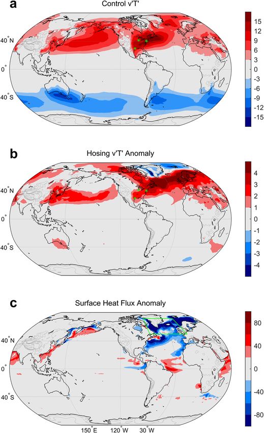
COMMUNICATIONS EARTH & ENVIRONMENT | https://doi.org/10.1038/s43247-021-00290-9 ARTICLE
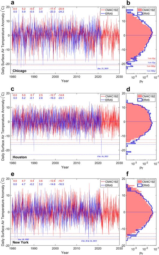
Next we focus on the U.S. daily surface air temperature (Ts) in
DJF. Compared with the reanalysis data of ERA540 during
1979–2021 (see “Methods” section), CM4C192 simulates the mean
and daily variations of Ts in DJF well in the control run
(Supplementary Fig. 6). As for extremely cold temperatures, we
evaluate the model performance at Chicago, Houston, and New
York, three large cities representing the Midwest, South, and
Northeast U.S., respectively. At Chicago, the daily temperature
anomaly relative to the daily climatology (ΔTs; see “Methods”
section) reached the lowest point of −23.5 °C on January 31, 2019 in
the detrended and deseasonalized ERA5 data (Fig. 3a, b). The
extremeness of the recent Texas cold snap during February 2021
(https://en.wikipedia.org/wiki/February_2021_North_American_
cold_wave) is even more striking. ΔTs at Houston plummeted to
−23.4 °C on February 16, 2021, by far colder than previous extreme
events (Fig. 3c, d). At New York, the coldest ΔTs occurred on January
18, 1982 and on February 20 and 24, 2015, with a magnitude of
about −16.3 °C (Fig. 3e, f).
At the three cities, CM4C192 simulates the general statistics of
ΔTs well in the control run, including its standard deviation,
skewness, and kurtosis (Fig. 3). However, the model under-
estimates extreme cold events as evidenced by the higher 10-year
10 100
and 100-year return levels (ΔT c and ΔT c ; see “Methods”
s s
section for the return level calculation), especially at Houston
(Fig. 3). Different resolutions and external forcings, as well as
existing model biases, are among the possible reasons for the
differences between the ERA5 data and CM4C192 simulations.
After the shutdown of AMOC in the hosing experiment, the
intensity and frequency of extremely cold daily temperatures over
the U.S. increase disproportionately compared with the mean
temperature response (Figs. 4 and 5 and Supplementary Fig. 7). At
Chicago, the 10-year and 100-year return levels of ΔT c 10 and ΔT
c 100
s s
further drop by 3.4 °C and 3.6 °C, respectively, in the hosing
experiment, compared with a mean cooling of 1.6 °C relative to the
100
control (Fig. 4a, b). ΔT c (−20.9 °C) in the control is almost
s
c 10 (−20.8 °C) in the hosing run, suggesting that the
identical to ΔT s
100-year extreme cold event could occur every 10 years at Chicago
after the AMOC shutdown. At Houston, ΔT c 100 drops more and by
s
4.6 °C from −14.8 °C in the control to −19.4 °C in the hosing
(Fig. 4c, d). It represents a change more than five times larger than
the mean cooling of 0.9 °C (Fig. 5f). Interestingly, this drop makes
c 100 in CM4C192 closer to that of ERA5 (Fig. 3c, d). At New
ΔT s
10 100
Fig. 1 Energy balance of the northern atmosphere in the climates with York, ΔTc c
and ΔT further drop by 5.6 °C and 5.4 °C,
s s
and without an active AMOC. a Schematic shows the energy balance for respectively, compared with a mean cooling of 2 °C (Fig. 4e, f).
the entire atmosphere north of 40°N. The left half with black numbers Extremely cold temperatures reaching or exceeding
100
(annual/DJF) shows heat fluxes (PW) at the top, bottom and southern c
ΔT s = −15.7 °C in the control occur more frequently and for
boundaries in the long-term control run of CM4C192. The right half with about 60 times/days in the hosing experiment.
red numbers shows the heat flux anomalies during years 21–100 of the To assess the uncertainty associated with the extreme value
hosing experiment relative to the control. The positive and negative values analysis, we perform the Kolmogorov–Smirnov test for the annual
indicate enhanced and reduced heat fluxes, respectively. Only the annual coldest ΔTs at Chicago, Houston and New York between the
mean value is shown for the oceanic transport. The blue and yellow control and hosing runs. The test rejects the null hypothesis at the
shadings denote the atmosphere and AMOC, respectively. b Annual 5% significance level that the control and hosing samples are drawn
northward heat transport by the global atmosphere and global ocean as from the same distribution. In terms of the return level estimate, we
a function of latitude in the control run. c Annual northward heat transport apply the bootstrap method to quantify its 90% confidence
of the global ocean and the Atlantic in the control and during years 21–100 bounds41 (Supplementary Fig. 8). The results confirm that
of the hosing experiment. The green vertical dashed line marks 40°N.
compared with the control, the drops of ΔT c 10 and ΔT c 100 in the
s s
relative to the control (Supplementary Fig. 5a). This global hosing experiment are statistically significant at the three cities.
cooling, centered at the northern North Atlantic, is a result of the
cloud, water vapor, and sea ice feedbacks associated with the Impact factors for the change in return levels. In the hosing
reduced northward heat transport in the ocean38,39. Other experiment, the drops in return level of extreme cold temperatures
changes of the large-scale mean climate in the hosing experiment could be caused by multiple factors42 (Fig. 5): the mean cooling,
are generally similar to the previous results1. increased overall variance, reduced skewness, changes in the
COMMUNICATIONS EARTH & ENVIRONMENT | (2021)2:218 | https://doi.org/10.1038/s43247-021-00290-9 | www.nature.com/commsenv 3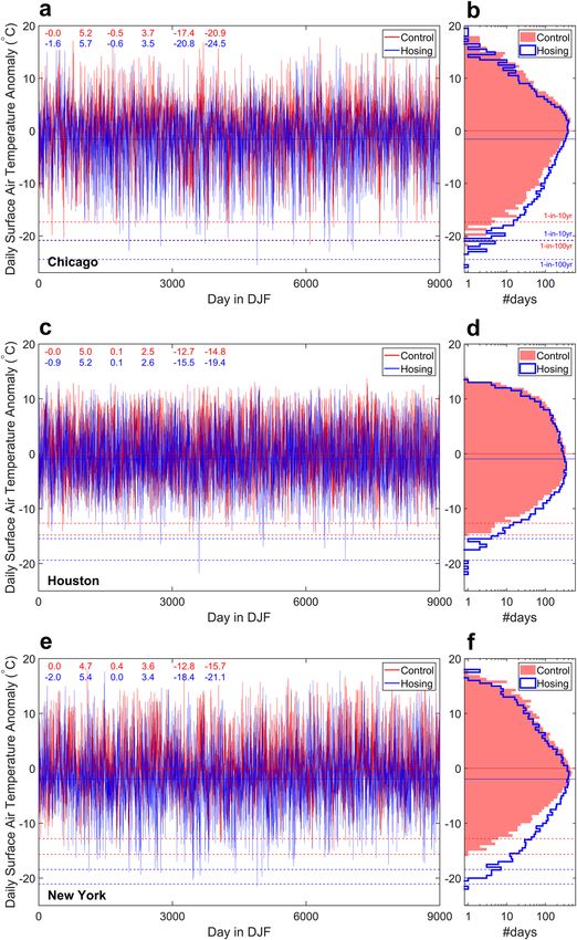
ARTICLE                                               COMMUNICATIONS EARTH & ENVIRONMENT | https://doi.org/10.1038/s43247-021-00290-9

Fig. 2 Enhanced atmospheric heat transport by transient eddies in response to the shutdown of AMOC. a Atmospheric eddy temperature flux (v′T′) (°C
m s−1) at 850 hPa in the long-term control. v′T′ is band passed using a Lanczos filter to identify synoptic variations on 3–15 days. Positive and negative
values indicate northward and southward transport of sensible heat, respectively. The green asterisks mark Chicago, Houston, and New York. The thin grey
lines are surface topography with 1000 m intervals. b Anomalies of the atmospheric eddy temperature flux (°C m s−1) during years 21–100 of the hosing
experiment relative to the control. c Anomalies of the surface heat flux (W/m2) during years 21–100 of the hosing experiment relative to the control.
Negative values indicate reduction of the upward heat flux. The freshwater perturbation is input into the ocean region of the green box. All values in
a, b and c are for DJF. See Supplementary Fig. 2 for the TOA and surface heat fluxes in the control run.

seasonal cycle (Supplementary Fig. 9), and individual extratropical           (Fig. 4e). Similarly, these factors are important to explain the
cyclones/anti-cyclones that become stronger and propagate more                intensification of extreme cold weather over western Europe (Fig. 5
southward. At New York, the mean cooling (−2.0 °C), the increased             and Supplementary Fig. 7), along with the increase in snow cover
standard deviation (from 4.7° to 5.4 °C) and the reduced skewness             (Supplementary Fig. 10). However, snow cover in the hosing
(from 0.4 to 0), as well as more extreme individual weather events,           experiment changes little over the U.S. due to a minimum cooling
                                  10         100
                               c and ΔT
all contribute to the drop of ΔT          c      in the hosing run            (Fig. 5a).
                                     s            s

4            COMMUNICATIONS EARTH & ENVIRONMENT | (2021)2:218 | https://doi.org/10.1038/s43247-021-00290-9 | www.nature.com/commsenv
COMMUNICATIONS EARTH & ENVIRONMENT | https://doi.org/10.1038/s43247-021-00290-9                                                          ARTICLE

Fig. 3 Data-model comparison of DJF daily temperature anomalies (ΔTs) at three cities of the U.S. a, b Chicago; c, d Houston; e, f New York. a, c, e The
time series for 1979–2021 of ERA5 and the 50-year control simulation of CM4C192. Both curves are detrended and deseasonalized so that the mean is
zero. The coldest value of ΔTs at each city in ERA5 is marked with its occurrence date. b, d, f The histograms of the 42-year ERA5 data and the 100-year
control simulation of CM4C192. Note that the x-axis uses a logarithmic scale and denotes probability (ci/N; ci—bin count; N—total count). The solid
horizontal lines show the mean. The dashed horizontal lines denote the return levels for the 1-in-10-year and 1-in-100-year cold events. Their values along
with the mean and three moments of the time series are listed at the upper left corner. From left to right: mean, standard deviation, skewness, kurtosis,
c 10 , and ΔT
ΔT         c 100 .
   s          s

COMMUNICATIONS EARTH & ENVIRONMENT | (2021)2:218 | https://doi.org/10.1038/s43247-021-00290-9 | www.nature.com/commsenv                                  5
ARTICLE                                                 COMMUNICATIONS EARTH & ENVIRONMENT | https://doi.org/10.1038/s43247-021-00290-9

Fig. 4 Response of DJF daily temperature anomalies (ΔTs) at three cities of the U.S. in the hosing experiment. a, b Chicago; c, d Houston; e, f New York.
a, c, e Time series for 100 years or 9000 DJF days. In both curves, the daily climatology from the control has been removed and the mean cooling remains
in the curve of the hosing run. b, d, f The histograms. The y-axis and x-axis are the temperature anomaly and the number of days, respectively. Note the
x-axis uses a logarithmic scale. The solid horizontal lines show the long-term mean. The dashed horizontal lines denote the return levels for the 1-in-10-year
and 1-in-100-year cold events. The statistics of the time series are listed at the upper left corner (from left to right: long-term mean, standard deviation,
skewness, kurtosis, ΔTc 10 and ΔT
                               c 100 ). These statistics are calculated based on years 1–100 of the control run and years 21–100 of the hosing run. The 90%
                         s 10     s 100
confidence bounds of ΔT   c and ΔT c      quantified by the bootstrapping can be found in Supplementary Fig. 8.
                           s         s

  By comparison, the drop of ΔT    c 10 and ΔT  c 100 at Houston is             related to the increased kurtosis, which also dominates the ratio
                                      s            s
mainly caused by individual extreme weather events rather than                  of the extreme and mean responses (Fig. 5d–f). The shutdown of
by the overall variability and skewness (Fig. 4c). This is consistent           AMOC sharpens the meridional temperature gradient at the
with the increase in kurtosis that measures the tailedness of the               northern mid-latitudes and increases the baroclinicity of the
temperature distribution (i.e., outliers). In fact, the large drops of          atmosphere. These lead to stronger weather systems that
c 100 in the Great Plains just east of the Rocky Mountains are
ΔT                                                                              propagate more southward.
    s

6            COMMUNICATIONS EARTH & ENVIRONMENT | (2021)2:218 | https://doi.org/10.1038/s43247-021-00290-9 | www.nature.com/commsenv
COMMUNICATIONS EARTH & ENVIRONMENT | https://doi.org/10.1038/s43247-021-00290-9 ARTICLE
Fig. 5 Changes in statistics of DJF daily temperature anomalies (ΔTs) over mid-latitude land areas in the hosing experiment. a Long-term mean (°C),
c 100 ; °C); f Ratio of the extreme (e) and mean (a) responses. The values show
b Standard deviation (°C), c Skewness, d Kurtosis, e 100-year return level (ΔT s
the changes in statistics during years 21–100 of the hosing experiment relative to the long-term control. f Large positive values over North America indicate
amplified responses of extremely cold daily temperature relative to the mean cooling. Negative values indicate that the extreme and mean temperature
responses have opposite signs. See Supplementary Fig. 7 for these statistics in the long-term control simulation.
It should be noted that the analysis above is based on daily of AMOC on extreme winter weather. Located at the upwind
temperature anomalies (ΔTs) relative to the daily climatology in direction of the North Atlantic, mean winter temperatures over
the control (T~ s ). Due to the relatively small curvature of the the U.S. are thought to be less influenced by the AMOC com-
seasonal cycle in DJF (Supplementary Fig. 9), the largest negative pared with the downwind European side (Fig. 5a and Supple-
anomalies also mean the local coldest weather during winter. mentary Fig. 3b). From a concise energy balance point of view
Among the three cities, Chicago is located in land interior and without involving much advanced atmospheric dynamics, we
generally colder than the coastal Houston and New York. The show here that AMOC can modulate daily temperature extremes
absolute daily temperature (Ts) at Chicago could drop to as low as more efficiently over the U.S. (Fig. 5e). The AMOC shutdown and
−27.4 °C in the hosing run of CM4C192, compared with the reduced northward heat transport in the Atlantic are capable of
coldest temperature of −14.3 °C at Houston and −21.6 °C at exciting more extremely cold weather over the U.S. during winter.
New York. This amplified response at the tail of the temperature distribution
could be several times larger than that of the mean (Fig. 5f).
Conclusions This sensitivity of extreme weather over land interior to deep
In this study, we use a state-of-the-art global weather/climate ocean circulation seems surprising but is nevertheless a robust
modeling system with high resolution to investigate the influence response required by Bjerknes compensation. Due to the
COMMUNICATIONS EARTH & ENVIRONMENT | (2021)2:218 | https://doi.org/10.1038/s43247-021-00290-9 | www.nature.com/commsenv 7ARTICLE COMMUNICATIONS EARTH & ENVIRONMENT | https://doi.org/10.1038/s43247-021-00290-9
north–south orientation of the mountain series over North Atmospheric and Oceanic heat transport. In this study, we use both the direct
America (Fig. 2), the Arctic outbreak during winter can push and indirect methods to calculate the heat transport by the atmosphere and ocean.
In the long-term control run, the total northward heat transport by the global
frigid polar air mass from Canada all the way southward to the atmosphere and global ocean at a latitude ϕ can be estimated by integrating the net
Gulf of Mexico. We find that this channel of intense atmospheric radiative flux at TOA from the South (or North) Pole to latitude ϕ.
heat exchange becomes even more active after the shutdown of Z ϕ Z 2π
AMOC, thereby intensifying extreme cold events over the U.S. In Qt ðϕÞ ¼ F TOA R2 cos ϕ0 dλ dϕ0 ð1Þ
π2
other words, an active AMOC in the present-day climate likely 0
makes the U.S. winter less harsh and extreme. Qt is the total northward heat transport; FTOA the net radiative flux at TOA; R
According to some of recent observational studies, the AMOC Earth’s radius; λ and ϕ are longitude and latitude, respectively. Similarly, the
atmospheric heat transport (Qa) is estimated as
has weakened during the past century43. In particular, the Z ϕ Z 2π
northward heat transport at 26°N in the North Atlantic reduced Qa ðϕÞ ¼ ðF TOA F sfc ÞR2 cosϕ0 dλ dϕ0 ; ð2Þ
by 0.17 PW and from 1.32 PW during 2004–2008 down to 1.15 π2 0
PW during 2009–2016, as a result of a recent AMOC slowdown where Fsfc is the heat flux at the surface.
event31. This reduction in ocean heat transport influenced the We adopt the direct method to calculate the heat transport in an ocean basin.
northern atmosphere through heat flux anomalies at the ocean Integrate the transport from the western to the eastern boundary and vertically.
surface. The magnitude of this reduction represents a sizeable Then sum across the ocean basins.
Z η Z e
fraction of that induced by the AMOC shutdown in the
Qo ðϕÞ ¼ ∑ ρw cp Tv R cosϕ dλ dz ð3Þ
CM4C192 simulations (Fig. 1). basin H w
Anyway, the model simulations carried out here represent a Qo is the global ocean heat transport, T the ocean potential temperature, v the
sensitivity study. Given the highly idealized nature of the hosing ocean meridional velocity, ρw seawater density, cp seawater heat capacity, η and H
experiment in this study, one should be cautious about its denote ocean surface and bottom, respectively.
implication for extreme cold weather in future climates. This is
evidenced by the opposite trends of the mean temperature and Sensible and latent heat fluxes from the atmospheric transient Eddies. To
calculate the atmospheric eddy heat fluxes, we apply a Lanczos bandpass filter46 to
Arctic sea ice between the ERA5 data and the daily atmospheric temperature (T), specific humidity (q), and meridional wind (v)
CM4C192 simulation (Supplementary Fig. 3). Compared with the to identify their variations on the synoptic timescale of 3–15 days. We first remove
shutdown case, in addition, a slowdown of AMOC could cause a the seasonal cycle before applying the filter to the time series.
similar but more gradual response of the extreme weather. L
Despite these caveats, one sure thing is that Bjerknes compen- x0ðtÞ ¼ ∑ wðkÞxðt kÞ ð4Þ
k¼L
sation, which is derived from the very basic law of energy
conservation, should continue to work in the future climate. wðkÞ ¼
sin2πf 2 k sin2πf 1 k sinπk=L
ð5Þ
Anything that alters one way of the energy flow will trigger a πk πk πk=L
response from the others.
k ¼ L; ¼ ; 0; ¼ ; L
x and x′ represent the original and filtered time series of T, q or v, respectively. f1
Methods and f2 are the cutoff frequencies for the bandpass filter. w(k) represents a set of
The GFDL CM4C192 model. CM4C192 is the high resolution version of the latest weights within the filter window (L = 25).
generation of the climate models developed and used at GFDL19. For various
metrics, it performs among the best CMIP6 models44. The atmospheric model
(AM4)20–22 adopts finite-volume cubed-sphere dynamical core with 192 grid boxes Analysis on extreme daily surface air temperature. The anomaly of daily sur-
per cube face (~0.5° grid spacing). It has 33 vertical levels and the model top is face air temperature is the departure from its daily climatology.
located at 1 hPa. The model incorporates updated physics such as a double-plume ~ s ðx; y; t 1 Þ; t 1 ¼ 1; 2; ¼ ; 365
ΔT s ðx; y; tÞ ¼ T s ðx; y; tÞ T ð6Þ
scheme for shallow and deep convection and a new mountain gravity wave drag
parameterization21. Due to improvements in model resolution, physics and ~ s and ΔTs are daily temperature, its climatology and anomaly, respectively. As
T s, T
dynamics, CM4C192 simulates strong synoptic systems well such as hurricanes45 ~ s over DJF
the coldest three months at the mid-latitude Northern Hemisphere, T
and atmospheric rivers22.
shows relatively small variation compared with the annual cycle (Supplementary
The oceanic model of CM4C192 is based on the Modular Ocean Model version ~ s in the
6 (MOM6)23. It uses the Arbitrary-Lagrangian-Eulerian algorithm in the vertical to Fig. 9). Note that ΔTs in the hosing experiment is calculated relative to T
allow for the combination of different vertical coordinates including geopotential control. So the change in the seasonal cycle (mean, amplitude and timing) in the
and isopycnal. The model adopts the C-grid stencil in the horizontal and is hosing run also contributes to ΔTs (Supplementary Fig. 9).
configured on a tripolar grid. It has a 0.25° eddy-permitting horizontal resolution To calculate return levels of extremely cold daily temperatures, we use the block
and 75 hybrid vertical layers down to the 6500 m maximum bottom depth. The maxima approach in the extreme value analysis41,47. We consider the time series of
vertical grid spacing can be as fine as 2 m near the ocean surface. −ΔTs and pick out the maximum daily values (i.e., the coldest daily temperatures)
Daily or even hourly data of important atmospheric variables are saved to in DJF for each year. Then we fit the generalized extreme value (GEV) distribution
facilitate analyses on weather and extreme events. These variables include surface to annual maxima of −ΔTs.
air temperature (Ts), precipitation, sea level pressure, atmospheric temperature (T) x μ 1k
at 250 and 850 hPa, zonal and meridional winds (u, v) at 250 and 850 hPa, and GðxÞ ¼ expf½1 þ k g ð7Þ
σ
specific humidity (q) at 850 hPa. The model uses a noleap calendar that has
365 days in every year. xμ
1þk >0
σ
Control run and water-hosing experiment with CM4C192. The initial condition k, σ, and μ are the shape, scale and location parameters of GEV, respectively. For
is obtained from a long-term control simulation under the 1850 radiative forcing. k = 0, the GEV distribution reduces to the Gumbel distribution. For k > 0 and k < 0,
During the 100-year control run under the 1950 radiative forcing, the global mean the GEV distribution becomes the Fréchet and Weibull distribution, respectively.
10 100
surface air temperature shows a slight increase (Supplementary Fig. 5a). This drift c and ΔT
After the three parameters are determined, the return levels (ΔT c ) can
s s
is mainly caused by some high-latitude regions. At low and mid-latitudes, Ts is be estimated with the inverse cumulative density function of the GEV distribution.
quite stable in the control run without any clear trend (Supplementary Fig. 5b–d). For example,
In the water-hosing experiment, a 0.6 Sv freshwater addition is input uniformly
c
100 σ 1 k
into the northern North Atlantic and the ocean region from 65°W–5°E and ΔT s ¼ μ f1 ½lnð1 Þ g ð8Þ
50°N–75°N (see the green box in Fig. 2c) for 100 years. This freshwater addition is k 100
not compensated elsewhere. So it leads to about 5 m global sea level rise over the To assess the uncertainty associated with the return level estimates and
100-year period. The perturbation freshwater is input at the same temperature as determine whether the changes in return level in the hosing experiment are
the local sea surface temperature. So while it is a mass source and reduces regional statistically significant, we use the bootstrap method41,48 to generate
and global ocean salinity, it is not a specific heat source or sink and therefore does 10,000 samples of the annual maximum values of −ΔTs and quantify the 90%
not influence the heat budget analysis here. confidence bounds.
8 COMMUNICATIONS EARTH & ENVIRONMENT | (2021)2:218 | https://doi.org/10.1038/s43247-021-00290-9 | www.nature.com/commsenvCOMMUNICATIONS EARTH & ENVIRONMENT | https://doi.org/10.1038/s43247-021-00290-9 ARTICLE
ERA5 reanalysis. ERA5 combines large amounts of historical observations and 21. Zhao, M. et al. The GFDL global atmosphere and land model AM4.0/LM4.0:
uses advanced modeling and data assimilation to obtain global estimates of the 2. Model description, sensitivity studies, and tuning strategies. J. Adv. Model.
atmosphere40. For the data-model comparison in this study, we use the 3-h global Earth Syst. 10, 735–769 (2018).
surface air temperature data from January 1, 1979 to February 28, 2021. The data 22. Zhao, M. Simulations of atmospheric rivers, their variability, and response to
with a 0.25° horizontal resolution are downloaded from the Copernicus Climate global warming using GFDL’s new high-resolution general circulation model.
Change Service (https://doi.org/10.24381/cds.adbb2d47). February 29 in the leap J. Clim. 33, 10287–10303 (2020).
years is removed before the data-model comparison. 23. Adcroft, A. et al. The GFDL global ocean and sea ice model OM4.0: model
description and simulation features. J. Adv. Model. Earth Syst. 11, 3167–3271
Data availability (2019).
The control simulation of GFDL CM4C192 can be found at the CMIP6 archive (https://
24. Doss-Gollin, J., Farnham, D. J., Lall, U. & Modi, V. How unprecedented was
esgf-node.llnl.gov/projects/cmip6/). ERA5 reanalysis data can be found at https://
the February 2021 Texas cold snap? Environ. Res. Lett. 16, 064056 (2021).
climate.copernicus.eu/climate-reanalysis. Supplementary Data 1–3 contain data that were 25. Busby, J. W. et al. Cascading risks: understanding the 2021 winter blackout in
used to generate Figs. 1, 3, and 4. Texas. Energy Res. Soc. Sci. 77, 102106 (2021).
26. Haarsma, R. J. et al. High resolution model intercomparison project
(HighResMIP v1. 0) for CMIP6. Geosci. Model Dev. 9, 4185–4208 (2016).
Code availability 27. Peixoto, J. P. & Oort, A. H. Physics of Climate (Springer, 1992).
The model codes can be found at https://www.gfdl.noaa.gov/coupled-physical-model- 28. Trenberth, K. E. & Caron, J. M. Estimates of meridional atmosphere and
cm4/. All other codes used in the analysis of this study are available from the ocean heat transports. J. Clim. 14, 3433–3443 (2001).
corresponding author upon request. 29. Fasullo, J. T. & Trenberth, K. E. The annual cycle of the energy budget. Part II:
Meridional structures and poleward transports. J. Clim. 21, 2313–2325 (2008).
30. Johns, W. E. et al. Continuous, array-based estimates of Atlantic Ocean heat
Received: 5 May 2021; Accepted: 23 September 2021; transport at 26.5N. J. Clim. 24, 2429–2449 (2011).
31. Bryden, H. L. et al. Reduction in ocean heat transport at 26N since 2008 cools
the eastern subpolar gyre of the North Atlantic Ocean. J. Clim. 33, 1677–1689
(2020).
32. Bjerknes, J. Advances in Geophysics Vol. 10, 1–82 (Elsevier, 1964).
33. Shaffrey, L. & Sutton, R. Bjerknes compensation and the decadal variability of
References the energy transports in a coupled climate model. J. Clim. 19, 1167–1181
1. Stouffer, R. J. et al. Investigating the causes of the response of the thermohaline (2006).
circulation to past and future climate changes. J. Clim. 19, 1365–1387 (2006). 34. Zhang, R. & Delworth, T. L. Impact of the Atlantic multidecadal oscillation on
2. Manabe, S. & Stouffer, R. J. The role of thermohaline circulation in climate. North Pacific climate variability. Geophys. Res. Lett. 34, 23 (2007).
Tellus B 51, 91–109 (1999). 35. Yang, H. et al. Heat transport compensation in atmosphere and ocean over the
3. Zhang, R. & Delworth, T. L. Simulated tropical response to a substantial past 22,000 years. Sci. Rep. 5, 1–11 (2015).
weakening of the Atlantic thermohaline circulation. J. Clim. 18, 1853–1860 36. Outten, S., Esau, I. & Ottera, O. H. Bjerknes compensation in the CMIP5
(2005). climate models. J. Clim. 31, 8745–8760 (2018).
4. Gregory, J. M. et al. A model intercomparison of changes in the Atlantic 37. Lutsko, N. J., Baldwin, J. W. & Cronin, T. W. The impact of large-scale
thermohaline circulation in response to increasing atmospheric CO2 orography on Northern Hemisphere winter synoptic temperature variability.
concentration. Geophys. Res. Lett. 32, L12703 (2005). J. Clim. 32, 5799–5814 (2019).
5. Vellinga, M. & Wood, R. A. Global climatic impacts of a collapse of the 38. Winton, M. On the climatic impact of ocean circulation. J. Clim. 16,
Atlantic thermohaline circulation. Clim. Change 54, 251–267 (2002). 2875–2889 (2003).
6. Rahmstorf, S. & Ganopolski, A. Long-term global warming scenarios computed 39. Herweijer, C., Seager, R., Winton, M. & Clement, A. Why ocean heat transport
with an efficient coupled climate model. Clim. Change 43, 353–367 (1999). warms the global mean climate. Tellus A 57, 662–675 (2005).
7. Levermann, A., Griesel, A., Hofmann, M., Montoya, M. & Rahmstorf, S. 40. Hersbach, H. et al. The ERA5 global reanalysis. QJRMS 146, 1999–2049
Dynamic sea level changes following changes in the thermohaline circulation. (2020).
Clim. Dyn. 24, 347–354 (2005). 41. Zwiers, F. W. & Kharin, V. V. Changes in the extremes of the climate
8. Yin, J., Schlesinger, M. E. & Stouffer, R. J. Model projections of rapid sea-level simulated by CCC GCM2 under CO2 doubling. J. Clim. 11, 2200–2222 (1998).
rise on the northeast coast of the United States. Nat. Geosci. 2, 262–266 (2009). 42. McKinnon, K. A., Rhines, A., Tingley, M. P. & Huybers, P. The changing
9. Jackson, L. et al. Global and European climate impacts of a slowdown of the shape of Northern Hemisphere summer temperature distributions. J. Geophys.
AMOC in a high resolution GCM. Clim. Dyn. 45, 3299–3316 (2015). Res. 121, 8849–8868 (2016).
10. Sigmond, M., Fyfe, J. C., Saenko, O. A. & Swart, N. C. Ongoing AMOC and 43. Caesar, L., McCarthy, G., Thornalley, D., Cahill, N. & Rahmstorf, S. Current
related sea-level and temperature changes after achieving the Paris targets. Atlantic Meridional overturning circulation weakest in last millennium. Nat.
Nat. Clim. Change 10, 672–677 (2020). Geosci. 118, 1–3 (2021).
11. Liu, W., Fedorov, A. V., Xie, S.-P. & Hu, S. Climate impacts of a weakened 44. Boucher, O. et al. Presentation and evaluation of the IPSL‐CM6A‐LR climate
Atlantic Meridional overturning circulation in a warming climate. Sci. Adv. 6, model. J. Adv. Model. Earth Syst. 12, e2019MS002010 (2020).
eaaz4876 (2020). 45. Murakami, H. et al. Detected climatic change in global distribution of tropical
12. Yin, J., Griffies, S. M., Winton, M., Zhao, M. & Zanna, L. Response of storm- cyclones. Proc. Natl Acad. Sci. USA 117, 10706–10714 (2020).
related extreme sea level along the US Atlantic coast to combined weather and 46. Duchon, C. E. Lanczos filtering in one and two dimensions. J. Appl. Meteorol.
climate forcing. J. Clim. 33, 3745–3769 (2020). Climatol. 18, 1016–1022 (1979).
13. Duchez, A. et al. Drivers of exceptionally cold North Atlantic Ocean 47. Coles, S., Bawa, J., Trenner, L. & Dorazio, P. An Introduction to Statistical
temperatures and their link to the 2015 European heat wave. Environ. Res. Modeling of Extreme Values (Springer, 2001).
Lett. 11, 074004 (2016). 48. Efron, B. The Jackknife, the Bootstrap and other Resampling Plans (SIAM,
14. Schenk, F. et al. Warm summers during the Younger Dryas cold reversal. Nat. 1982).
Commun. 9, 1–13 (2018).
15. Rousi, E., Selten, F., Rahmstorf, S. & Coumou, D. Changes in North Atlantic
atmospheric circulation in a warmer climate favor winter flooding and Acknowledgements
summer drought over Europe. J. Clim. 34, 2277–2295 (2021). We thank Ron Stouffer, Zhihong Tan, and two reviewers for their comments, and
16. Bryden, H. L., King, B. A., McCarthy, G. D. & McDonagh, E. L. Impact of a ECMWF and the Copernicus Climate Change Service for providing the ERA5 reanalysis
30% reduction in Atlantic meridional overturning during 2009–2010. Ocean data. The work is supported by the NOAA Climate Program Office (Grant #
Sci. 10, 683–691 (2014). NA18OAR4310267).
17. Hallam, S. et al. Ocean precursors to the extreme Atlantic 2017 hurricane
season. Nat. Commun. 10, 1–10 (2019).
18. Woollings, T., Gregory, J. M., Pinto, J. G., Reyers, M. & Brayshaw, D. J. Author contributions
Response of the North Atlantic storm track to climate change shaped by J.Y. initiated the idea and M.Z. carried out the CM4C192 simulations. J.Y. led the data
ocean–atmosphere coupling. Nat. Geosci. 5, 313–317 (2012). analysis and manuscript writing. Both discussed the results and contributed to the
19. Held, I. M. et al. Structure and performance of GFDL’s CM4.0 climate model. improvement of the manuscript.
J. Adv. Model. Earth Syst. 11, 3691–3727 (2019).
20. Zhao, M. et al. The GFDL global atmosphere and land model AM4.0/LM4.0:
1. Simulation characteristics with prescribed SSTs. J. Adv. Model. Earth Syst. Competing interests
10, 691–734 (2018). The authors declare no competing interests.
COMMUNICATIONS EARTH & ENVIRONMENT | (2021)2:218 | https://doi.org/10.1038/s43247-021-00290-9 | www.nature.com/commsenv 9ARTICLE COMMUNICATIONS EARTH & ENVIRONMENT | https://doi.org/10.1038/s43247-021-00290-9
Additional information Open Access This article is licensed under a Creative Commons
Supplementary information The online version contains supplementary material Attribution 4.0 International License, which permits use, sharing,
available at https://doi.org/10.1038/s43247-021-00290-9. adaptation, distribution and reproduction in any medium or format, as long as you give
appropriate credit to the original author(s) and the source, provide a link to the Creative
Correspondence and requests for materials should be addressed to Jianjun Yin. Commons license, and indicate if changes were made. The images or other third party
material in this article are included in the article’s Creative Commons license, unless
Peer review information Communications Earth & Environment thanks Fuyao Wang
indicated otherwise in a credit line to the material. If material is not included in the
and the other, anonymous, reviewer(s) for their contribution to the peer review of this
article’s Creative Commons license and your intended use is not permitted by statutory
work. Primary Handling Editor: Heike Langenberg.
regulation or exceeds the permitted use, you will need to obtain permission directly from
the copyright holder. To view a copy of this license, visit http://creativecommons.org/
Reprints and permission information is available at http://www.nature.com/reprints
licenses/by/4.0/.
Publisher’s note Springer Nature remains neutral with regard to jurisdictional claims in
published maps and institutional affiliations. © The Author(s) 2021
10 COMMUNICATIONS EARTH & ENVIRONMENT | (2021)2:218 | https://doi.org/10.1038/s43247-021-00290-9 | www.nature.com/commsenvYou can also read