International Journal of Multidisciplinary Approach - Weather Atmospheric Electric ...
←
→
Page content transcription
If your browser does not render page correctly, please read the page content below
International Journal of Multidisciplinary Approach
                and Studies                                              ISSN NO:: 2348 – 537X

   Effect of Orography on Fair - Weather Atmospheric Electric
                  Field in Kashmir Valley, India.
             Shaista Afreen*, Gowher Bashir**, Nissar Ahmed***.
             Department of Physics, University of Kashmir, Hazratbal, J&K, 190006, India.

ABSTRACT:

Atmospheric electric parameters like electric field change with orography of earth’s surface
due to changes in ionisation rates, radioactivity and concentration of cloud condensation
nuclei changes with altitude of a place. This work presents atmospheric electric field of three
different sites in Kashmir valley which have been calculated theoretically and measured
experimentally. Fair weather conditions were taken into account for both while selecting
data for observational results and calculating the values theoretically. The results obtained
of both are in accordance with each other, thus, verifying that orography plays an important
role in determining the atmospheric electric field.

KEYWORDS: Electric field, Fair- weather, Orography.

INTRODUCTION:

The atmospheric electrical parameters have been studied by a lot of researchers for a long
period of time over various locations of globe. These parameters depend on factors such as
thunderclouds, meteorological factors, solar activity and pollution. The PG shows a diurnal
variation which closely follows the pattern of world thunderstorm activity. This was used to
formulate the global electric circuit. Atmospheric electric parameters like potential gradient
and air- earth current density can be explained by diurnal variation of thunderstorms whereas
parameters like conductivity is influenced by formation and recombination/ attachment rate
of ions (Making & Ogawa, 1984).
The lower troposphere region of the atmosphere, upto height of 9 km, is the most important
region while considering the effect of orography on atmospheric electric parameters. The
electrical conductivity changes with altitude (Agarwal & Varshneya, 1993) due to varying
ionisation rates because of the orography of the earth’s surface (Srinivas & Prasad, 1993).
Ionisation caused mainly due to radioactivity of earth is destroyed due to adhesion to large
nuclei. Atmospheric electric parameters like conductivity and current density increase with
height from sea level while electric field decreases. This happens because parameters like
ionisation due to cosmic rays, radioactivity etc. varies with altitude of a place. Also, the
concentration of cloud condensation nuclei increases with altitude of a place, thus
                                                                                                   37

mountainous regions have higher cloud condensation nuclei than the plains (Siingh et al.,
                                                                                                   Page :

2007).
Solar flares and coronal mass ejections (CMEs) from sun release lots of highly energetic
particles. If they are in right position, these can interact with earth’s atmosphere (Dickinson,
1975) via the solar wind and interplanetary magnetic field and be known as solar proton

Volume 08, No.1, Jan – Feb 2021
International Journal of Multidisciplinary Approach
and Studies ISSN NO:: 2348 – 537X
event. These energetic particles interact with earth’s lower and middle atmosphere causing
ionisation up to about 60 km from earth’s surface(Baumgaertner et al., 2013) or by affecting
nucleation of water drops to form clouds(Rycroft et al., 2000). The layer of atmosphere from
60km to 300 km is known as ionosphere. This process has very important role in ionisation
on earth’s surface and thus the GEC. Therefore, it can be expected that the atmospheric
electrical parameters will be influenced by solar activity.(Hays & Roble, 1979) using a quasi-
static model calculated that changes in conductivity due to solar flares can affect the global
electric circuit. The atmospheric electric field increases during solar flares in mountainous
regions (Makino & Ogawa, 1985).
Kumar et al., (1998) did a theoretical study of variation of atmospheric electric parameters
with orography for 39 cities of India assuming fair weather conditions. They found that
conductivity of places with altitude greater than 2100m was higher than places with lower
altitude. They found conductivity decreases linearly with decrease in altitude and that the
orographic effect is much higher than the latitudinal effect. This was found to be in
accordance with result of Agarwal & Varshneya, (1993). The values of electric filed
calculated by Kumar et al., (1998) also verified the effect of orography on electric field. The
electric field of mountainous regions like Shillong, Shimla, Srinagar etc. were found to be
lower (~ 105 Vm-1) whereas places close to sea level had higher values of electric field (~
110 Vm-1).
Kumar & Singh, (2013) also found a similar increase in conductivity and corresponding
decrease in electric field with increasing altitude calculated for 80 orographically different
places of India. They took the cosmic ray modulation factor due to forbusch decrease into
consideration.
Saxena et al., (2010) collected geographical data for 160 places of US and calculated
atmospheric electric parameters like conductivity, air earth current, electric field and
potential. The electrical conductivity and current density increases exponentially with
altitude. They further reportedthat electric field value remains constant with a value of 112.42
Vm-1 while electric potential decreases with increasing height with values ranging between
267.96 kV to 290.34 kV.
It appears that all the workers have attempted to study the effect of orography on atmospheric
electricity on a theoretical basis and to the author’s knowledge, no study verifies it
experimentally. So the authors have conducted a study at 3 different places in Kashmir valley
and the results thereof have been presented.
Site description:
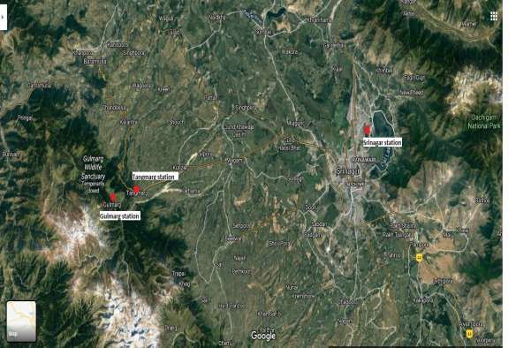
The Kashmir valley is surrounded on the south-western side by the Pir Panjal Range and on
the north-eastern side by the main Himalayas. A majority of the valley’s topography is
mountainous, and is divided into 7 zones which are: the plains, foothills, Pir Panjal, Vale of
Kashmir, Great Himalayas, Indus river valley and the Karakoram. In order to observe the
38
effect of orography on electric field three sites from Kashmir valley were chosen for study:
Srinagar, Tangmarg and Gulmarg.The stations are marked in the topographical map of
Page :
Kashmir valley (Figure 1).
Srinagarstation is located at an altitude of 1585 metres above mean sea level and has the
coordinates (34° 13’ N, 74° 83’ E). Srinagar city is situated in the centre of Kashmir valley
Volume 08, No.1, Jan – Feb 2021International Journal of Multidisciplinary Approach
and Studies ISSN NO:: 2348 – 537X
and is the summer capital of union territory of Jammu and Kashmir. The field mill (EFM
100) is installed in the University of Kashmir which lies on the north-eastern bank of world
famous Dal lake and has Nigeen lake on the western side. This area is typically of urban
nature but does not have any large scale factories and industries nearby. Also, vehicular
movement is restricted in the university campus.
The site of Tangmarg station is located at an altitude of about 2080 metres above mean sea
level and has the coordinates (34° 06’ N, 74° 39’ E). This site is rural in nature and is hilly.
Most of its area is covered by forests.
The Gulmarg site is located at an high altitude of about 2617.2 meters above mean sea level
and has the coordinates (34°05’N and 74°42’E).It lies in the Pir Panjal range and the site is
covered by lush green meadows surrounded by green forests of pine and fir. There is no
permanent population around the observatory.
All the sites record a temperate climate with temperatures not exceeding about 33° C in
summers. Winters are cold in all the stations with sub-zero temperatures recorded during
nights. Severe cold conditions are recorded especially in Gulmarg where ground is covered in
thick layers of snow for five months of the year. All the observations were carried on fair
weather days i.e. days with no precipitation, no local thunderstorms, and clear skies. Sites for
observation were chosen carefully with no tall building, trees or electric poles nearby.
RESULTS AND DISCUSSION:
In this work, we have calculated the atmospheric electric field theoretically for the three
chosen sites in Kashmir valley and compared our results with experimental values.
The electrical conductivity of a place is given by the equation
Ϭ (z,θ) = ϭS1 exp[z/2S1(θ)] Sm-1 (1)
where z is the height from sea level
θ is the co-latitude
ϭS1 is the sea level conductivity = 2.2 ×10⁻¹⁴ Sm-1
S1(θ) is the conductivity scale height
The conductivity scale height is given by the equation
S1(θ) = z1/ {2 ln [(ϭr(θ)/ϭS1) exp(z1/2S2)]} km (2)
where z1 is the height of boundary layer separating upper and lower troposphere = 9 km
ϭr(θ) is the reference conductivity
S2 is the scale height of vertical variation of conductivity = 3 km
The reference conductivity is calculated using equation
ϭr(θ) = ϭ0 [1+(∆F/2) {1+cos3(θ- 30)}] Sm-1(3)
39
whereϭ0 is the reference conductivity at equator = 1.1 ×10⁻¹³
∆F is the latitude variation factor due to cosmic rays =0.4
Page :
The columnar resistance, Rc(θ) between the ionosphere and earth’s surface is given as the
sum of columnar resistance between ground (zg) and boundary between lower and upper
troposphere (z1) (Rc1 (θ)); and z1 and ionosphere (zi) (Rc2 (θ)). Hence,
Volume 08, No.1, Jan – Feb 2021International Journal of Multidisciplinary Approach
and Studies ISSN NO:: 2348 – 537X
Rc(θ) = Rc1 (θ)+ Rc2 (θ) Ωm2 (4)
where
Rc1 (θ) = Ωm2
and
Rc2 (θ) = Ωm2
The air-earth current is given by
(5)
where is the ionospheric potential = 300 kV
Then, the electric field E(z,θ) can be calculated as
J (z, θ) = E(z, θ) ×ϭ (z, θ) Am-2 (6)
Using the equations 1 to 6, the values of all the parameters were calculated theoretically and
are tabulated in table 1. The parameters calculated have been plotted in figure 2.
As an example the calculations for Srinagar station are shown below:
Reference conductivity has been calculated using equation (3):
ϭr(θ) = (1.1× 10⁻¹³) (1+0.2 (1+cos3(55.87-30))
=(1.1× 10⁻¹³) (1+0.2 (1.209))
=1.365×10⁻¹³ Sm-1
Substitute in equation (2) to calculate the conductivity scale height:
S1(θ)= 9/2 ln[(1.365×10⁻¹³/2.2×10-14). exp(9/6)]
=1.352 km
Substitute the above value in equation (1) to calculate electrical conductivity:
Ϭ (z,θ)= (2.2×10⁻¹⁴). exp(1585/2× 1352.28)
= 3.95×10⁻¹⁴ Sm-1
The columnar resistance Rc(θ) is calculated using equation (4):
Rc(θ) = Rc1 (θ)+ Rc2 (θ) Ωm2
Rc (θ) = dz
+ dz
=639.86×10¹⁴+44.04×10¹⁴
40
= 683.9×10¹⁴ Ωm2
Page :
Using above value in equation (5), the air- earth current density can be calculated as:
= 3,00,000/ 683.9×1014
= 4.386×10⁻¹² Am-2
Volume 08, No.1, Jan – Feb 2021International Journal of Multidisciplinary Approach
and Studies ISSN NO:: 2348 – 537X
Substituting the value of J (z, θ) and ϭ (z, θ) in equation (6), we get the value of electric field,
E(z, θ) as
E(z, θ)= J (z, θ)/ ϭ (z, θ)
= 4.386×10⁻¹²/ 3.95×10-14
= 111.03 Vm-1
To measure the values of atmospheric electric field at ground surface an electric field mill
(EFM 100) was used. In Srinagar station, the field mill was installed on a roof top with height
5.4m from the ground which led to an increase in the electric field values. So, a correction
factor was calculated by placing the mill flush with the ground. The values of electric field
were then corrected by multiplying with this correction factor. The average electric field was
found to be 148.54 Vm-1. In Gulmarg station, the electric field mill was placed at a height of
about 4m from the ground surface and a correction factor was calculated in a similar manner
to Srinagar station. The average value of electric field observed was 111.21 Vm-1. At
Tangmarg station the field mill was placed was placed at ground surface, so no correction
factor needed to be calculated and the average value of electric field was 113 Vm-1. These
results have been plotted in figure 3.
There seems to be a good correlation between the theoretical and observed values of electric
field except for Srinagar station where observed values are higher than theoretical values
which can be attributed to relatively higher amount of pollution at the station. Aerosols are
capable of modifying the electric field of atmosphere by acting as a platform for
recombination of ions leading to ion loss. In addition, pollutants lower the ion mobility,
reducing the conductivity, thus increasing potential gradient (Harrison & Carslaw, 2003;
Williams, 2003).
CONCLUSION:
The good agreement between theoretically calculated and observed values proves that
orography of a place plays a very important role in fair weather atmospheric electric field.
ACKNOWLEDGEMENT:
The authors are thankful to the University Grant Commission- SAP (File No.: F.530/15/DRS-
1/2016 (SAP-1); Dated: Feb 2016) for funding for the project.
REFERENCES:
i. Agarwal, R., & Varshneya, N. (1993). Global electric circuit parameters over Indian
subcontinent. Indian Journal of Radio & Space Physics (IJRSP).
41
ii. Baumgaertner, A. J. G., Thayer, J. P., Neely, R. R., & Lucas, G. (2013). Toward a
Page :
comprehensive global electric circuit model: Atmospheric conductivity and its
variability in CESM1(WACCM) model simulations. Journal of Geophysical Research
Atmospheres. https://doi.org/10.1002/jgrd.50725
iii. Dickinson, R. E. (1975). Solar Variability and the Lower Atmosphere. Bulletin of the
Volume 08, No.1, Jan – Feb 2021International Journal of Multidisciplinary Approach
and Studies ISSN NO:: 2348 – 537X
American Meteorological Society. https://doi.org/10.1175/1520-
0477(1975)0562.0.co;2
iv. Harrison, R. G., & Carslaw, K. S. (2003). Ion-aerosol-cloud processes in the lower
atmosphere. Reviews of Geophysics. https://doi.org/10.1029/2002RG000114
v. Hays, P. B., & Roble, R. G. (1979). A quasi-static model of global atmospheric
electricity, 1. The lower atmosphere. Journal of Geophysical Research.
https://doi.org/10.1029/ja084ia07p03291
vi. Kumar, A., Rai, J., Nigam, M. J., Singh, A. K., & Nivas, S. (1998). Effect of orographic
features on atmospheric electrical parameters of different cities of India. Indian Journal
of Radio and Space Physics.
vii. Kumar, A., & Singh, H. P. (2013). Impact of High Energy Cosmic Rays on Global
Atmospheric Electrical Parameters over Different Orographically Important Places of
India. ISRN High Energy Physics. https://doi.org/10.1155/2013/831431
viii. Making, M., & Ogawa, T. (1984). Responses of atmospheric electric field and air-earth
current to variations of conductivity profiles. Journal of Atmospheric and Terrestrial
Physics. https://doi.org/10.1016/0021-9169(84)90087-4
ix. Makino, M., & Ogawa, T. (1985). Quantitative estimation of global circuit. Journal of
Geophysical Research. https://doi.org/10.1029/JD090iD04p05961
x. Rycroft, M. J., Israelsson, S., & Price, C. (2000). The global atmospheric electric circuit,
solar activity and climate change. Journal of Atmospheric and Solar-Terrestrial Physics.
https://doi.org/10.1016/S1364-6826(00)00112-7
xi. Saxena, D., Yadav, R., & Kumar, A. (2010). Effect of orographic features on global
atmospheric electrical parameters over 160 different places of United States. Indian
Journal of Physics. https://doi.org/10.1007/s12648-010-0022-2
xii. Siingh, D., Gopalakrishnan, V., Singh, R. P., Kamra, A. K., Singh, S., Pant, V., Singh,
R., & Singh, A. K. (2007). The atmospheric global electric circuit: An overview.
Atmospheric Research. https://doi.org/10.1016/j.atmosres.2006.05.005
xiii. Srinivas, N., & Prasad, B. (1993). Seasonal-and latitudinal variations of stratospheric
small ion density and conductivity. Indian Journal of Radio & Space Physics (IJRSP).
xiv. Williams, E. R. (2003). Comment to “Twentieth century secular decrease in the
atmospheric potential gradient” by Giles Harrison. Geophysical Research Letters.
https://doi.org/10.1029/2003GL017094
42
Page :
Volume 08, No.1, Jan – Feb 2021International Journal of Multidisciplinary Approach
and Studies ISSN NO:: 2348 – 537X
Tables:
Station Latitude Longitude Height Conductivity Current Electric
from sea ×10-14 Sm-1 density field
level (m) ×10-12 Am-2 Vm-1
Srinagar 34° 13’ N 74° 83’ E 1585 3.95 4.386 111.03
Tangmarg 34° 06’ N 74° 39’ E 2080 4.80 5.24 109.1
Gulmarg 34° 05’ N 74° 42’ E 2617.2 5.86 6.34 108.1
Table 1: Calculated values of atmospheric electric parameters of the three stations of Kashmir
valley considering fair weather conditions.
Figure legends:
Figure 1: Topographical map of Kashmir valley showing the location of three stations.
Figure 2: Calculated atmospheric electric parameters for three stations in Kashmir valley.
Figure 3: Observed electric field values for the three stations in Kashmir valley.
43
Figure 1: Topographical map of Kashmir valley showing the location of three stations.
Page :
Volume 08, No.1, Jan – Feb 2021International Journal of Multidisciplinary Approach
and Studies ISSN NO:: 2348 – 537X
Figure 2: Calculated atmospheric electric parameters for three stations in Kashmir
valley.
44
Page :
Figure 3: Observed electric field values for the three stations in Kashmir valley.
Volume 08, No.1, Jan – Feb 2021You can also read