Introduction to scikit-learn - Georg Zitzlsberger 26-03-2021
←
→
Page content transcription
If your browser does not render page correctly, please read the page content below

Introduction to scikit-learn

Georg Zitzlsberger   georg.zitzlsberger@vsb.cz

26-03-2021

Agenda

What is scikit-learn?

Classification

Regression

Clustering

Dimensionality Reduction

Model Selection

Pre-Processing

What Method is the Best for Me?
What is scikit-learn?

I Simple and efficient tools for predictive data analysis
     I Machine Learning methods
     I Data processing
     I Visualization
I Accessible to everybody, and reusable in various contexts
     I Documented API with lot’s of examples
     I Not bound to Training frameworks (e.g. Tensorflow, Pytorch)
     I Building blocks for your data analysis
I Built on NumPy, SciPy, and matplotlib
     I No own data types (unlike Pandas)
     I Benefit from NumPy and SciPy optimizations
     I Extends the most common visualisation tool
I Open source, commercially usable - BSD license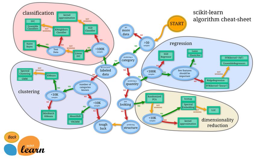
Tools of scikit-learn
I Classification:
  Categorizing objects to one or more classes.
    I   Support Vector Machines (SVM)
    I   Nearest Neighbors
    I   Random Forest
    I   ...
I Regression:
  Prediction of one (uni-) or more (multi-variate)
  continuous-valued attributes.
    I   Support Vector Regression (SVR)
    I   Nearest Neighbors
    I   Random Forest
    I   ...
I Clustering:
  Group objects of a set.
    I   k-Means
    I   Spectral Clustering
    I   Mean-Shift
    I   ...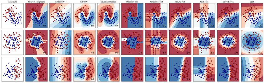
Tools of scikit-learn - cont’d
I Dimensionality reduction:
  Reducing the number of random variables.
    I   Principal Component Analysis (PCA)
    I   Feature Selection
    I   non-Negative Matrix Factorization
    I   ...
I Model selection:
  Compare, validate and choose parameters/models.
    I Grid Search
    I Cross Validation
    I ...
I Pre-Processing:
  Prepare/transform data before training models.
    I   Conversion
    I   Normalization
    I   Feature Extraction
    I   ...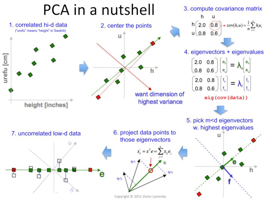
User Guide

The User Guide can be found   here
Choosing the Right Estimator

                                 (Image: scikit-learn.org)

Linked map can be found   here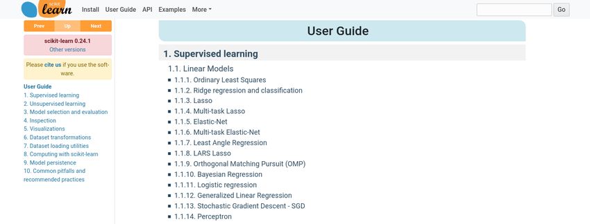
How to Get scikit-learn

 I Open Source (BSD License) available on   Github

 I Current version: 0.24.2
 I Easy install via PIP or Conda for Windows, macOS and Linux, e.g:
   $ pip install scikit-learn or
   $ conda install -c intel scikit-learn
Programming Model
 I Builds on NumPy, SciPy and matplotlib:
      I Avoids conversion of data types
      I Can be integrated seamlessly, even with Tensorflow and Pytorch
      I Benefits from performance optimizations of BLAS, FFT, etc. optimizations
 I scikit-learn available as Python module:

    import sklearn
    sklearn . show_versions ()

    System :
        python : 3.8.6 | packaged by conda - forge | ( default , Dec 26 2020 , 05:05:16)   [ GCC 9.3.0]
    executable : / opt / conda / bin / python
       machine : Linux -3.10.0 -1127.13.1. el7 . x86_64 - x86_64 - with - glibc2 .10

    Python dependencies :
              pip : 20.3.3
       setuptools : 49.6.0. post20201009
          sklearn : 0.24.0
            numpy : 1.19.5
            scipy : 1.5.3
           Cython : 0.29.21
           pandas : 1.1.5
       matplotlib : 3.3.3
           joblib : 1.0.0
    threadpoolctl : 2.1.0

    Built with OpenMP : True

 I Typical input (n samples, n features), but others are also possible
Example Datasets
 I Easy access to       ”toy” datasets   via sklearn.datasets:
     I   Boston house prices dataset
     I   Iris plants dataset
     I   Diabetes dataset
     I   Optical recognition of handwritten digits dataset
     I   Linnerrud dataset
     I   Wine recognition dataset
     I   Breast cancer wisconsin (diagnostic) dataset
 I Loading via:
      Function                                             Description
      load boston(*[, return X y])                         Load and return     the boston house-prices dataset
                                                           (regression).
      load   iris(*[, return X y, as frame])               Load and return     the   iris dataset (classification).
      load   diabetes(*[, return X y, as frame])           Load and return     the   diabetes dataset (regression).
      load   digits(*[, n class, return X y, as frame])    Load and return     the   digits dataset (classification).
      load   linnerud(*[, return X y, as frame])           Load and return     the   physical excercise linnerud dataset.
      load   wine(*[, return X y, as frame])               Load and return     the   wine dataset (classification).
      load   breast cancer(*[, return X y, as frame])      Load and return     the   breast cancer wisconsin dataset
                                                           (classification).
Using Example Datasets
I Convention:
I X: Data for training/prediction
I y: Label in case of supervised learning
(aka. target)
I n class: How many classes from the set
should be retrieved
I return X y: Boolean whether tuple of data
and label is desired
I as frame: Boolean whether data should be a
Pandas DataFrame
I Example:
import sklearn . datasets
sk_digits = sklearn . datasets . load_digits ( n_class =2 ,
return_X_y = True ,
as_frame = False )
print ( sk_digits )
( array ([[ 0. , 0. , 5. , ... , 0. , 0. , 0.] ,
... ,
[ 0. , 0. , 6. , ... , 6. , 0. , 0.]]) ,
array ([0 , 1 , 0 , 1 , 0, 1, 0, 0,
... ,
1, 1, 1, 1, 1 , 0 , 1 , 0]))Classification
I Supervised:
Label information is available and can be used for learning
I Unsupervised:
No (initial) labels and learning needs to structure data on its own
I Many classification methods exist:
From scikit-learn documentation: Classifier comparisonRegression
I Classification vs. Regression1 :
I Classify for categorical output
I Regression: predicting continuous-valued attribute(s)
I Can be ”by-products” of classification methods, e.g.:
RandomForestClassifier and RandomForestRegressor, or
SVC and SVR
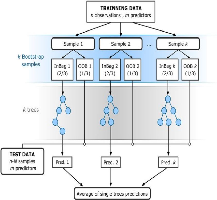
1 As scikit-learn regards it.Regression Example: Random Forest
I Ensemble of decision trees
I Perturb-and-combine technique applied to trees
I Considers diverse set of classifiers
I Randomization is achieved by selection of different
classifiers
I Prediction is majority vote or average over all trees
I Easily extends to multi-output problems
Modelling interannual variation in the spring and autumn land surface
phenology of the European forest, Rodriguez-Galiano, et al.
Process Variable Importance Analysis by Use of Random Forests in a
Shapley Regression Framework, AldrichRandom Forest Example
import numpy as np # Plot the results
import matplotlib . pyplot as plt plt . figure ()
from sklearn . ensemble import R a n d o m F o r e s t R e g r e s s o r s = 50
from sklearn . mo de l _s el ec t io n import tr a i n _ t e s t _ s p l i t a = 0.4
from sklearn . multioutput import M u l t i O u t p u t R e g r e s s o r plt . scatter ( y_test [: , 0] , y_test [: , 1] , edgecolor = ’k ’ ,
c = " navy " , s =s , marker = " s " , alpha =a , label = " Data " )
plt . scatter ( y_multirf [: , 0] , y_multirf [: , 1] , edgecolor = ’k ’ ,
# Create a random dataset c = " cornfl owerblue " , s =s , alpha =a ,
rng = np . random . RandomState (1) label = " Multi ␣ RF ␣ score =%.2 f " % regr_multirf . score ( X_test ,
X = np . sort (200 * rng . rand (600 , 1) - 100 , axis =0) y_test ))
y = np . array ([ np . pi * np . sin ( X ). ravel () , plt . scatter ( y_rf [: , 0] , y_rf [: , 1] , edgecolor = ’k ’ ,
np . pi * np . cos ( X ). ravel ()]). T c = " c " , s =s , marker = " ˆ " , alpha =a ,
y += (0.5 - rng . rand (* y . shape )) label = " RF ␣ score =%.2 f " % regr_rf . score ( X_test , y_test ))
plt . xlim ([ -6 , 6])
X_train , X_test , y_train , y_test = t r a i n _ t e s t _ s p l i t ( plt . ylim ([ -6 , 6])
X , y , train_size =400 , test_size =200 , random_state =4) plt . xlabel ( " target ␣ 1 " )
plt . ylabel ( " target ␣ 2 " )
max_depth = 30 plt . title ( " Comparing ␣ random ␣ forests ␣ and ␣ the ␣ multi - output ␣ " +
regr_multirf = M u l t i O u t p u t R e g r e s s o r ( " meta ␣ estimator " )
R a n d o m F o r e s t R e g r e s s o r ( n_estimators =100 , plt . legend ()
max_depth = max_depth , plt . show ()
random_state =0))
regr_multirf . fit ( X_train , y_train )
regr_rf = R a n d o m F o r e s t R e g r e s s o r ( n_estimators =100 ,
max_depth = max_depth ,
random_state =2)
regr_rf . fit ( X_train , y_train ) Python source code:
# Predict on new data Random Forest Regression
y_multirf = regr_multirf . predict ( X_test )
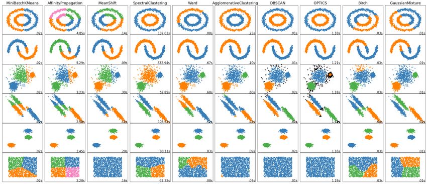
y_rf = regr_rf . predict ( X_test )Clustering I Many clustering methods exist: From scikit-learn documentation: Clustering comparison
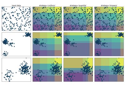
Clustering
 I Unsupervised: Find clusters (set of classes) automatically
 I Clustering is applied in two steps:
     1. Train (i.e. identify) cluster with training data
     2. Retrieve the labels/metrics from the trained model

                                                                Table can be found
                                                                in documentation
Dimensionality Reduction I Richard Bellman: The Curse of Dimensionality The curse of dimensionality refers to various phenomena that arise when analyzing and organizing data in high-dimensional spaces that do not occur in low-dimensional settings such as the three-dimensional physical space of everyday experience. I On the other hand, we want to work within dimensions as low as possible that still show the same/similar variance.
Dimensionality Reduction Example: PCA

 I Principal Component Analysis (PCA):
     I Batched PCA
     I Mini-batch like IncrementalPCA
     I PCA with randomized Singular Value
       Decomposition
       (svd solver=’randomized’)
     I Kernel based PCA KernelPCA
       (e.g. RBF, polynomial, sigmoid)
 I For some methods PCA might be a
   pre-requisite, e.g. SVM, K-Means
 I Note that PCA looses information!        https://devopedia.org/principal- component- analysis
PCA Example: PCA with Randomized SVD
import logging plot_gallery ( " First ␣ centered ␣ Olivetti ␣ faces " ,
from time import time face s_center ed [: n_components ])
from numpy . random import RandomState
import matplotlib . pyplot as plt estimator = decomposition . PCA ( n_components = n_components ,
from sklearn . datasets import f e t c h _ o l i v e t t i _ f a c e s svd_solver = ’ randomized ’ ,
from sklearn import decomposition whiten = True )
t0 = time ()
n_row , n_col = 2 , 3 data = faces
n_components = n_row * n_col data = fac es_cente red
image_shape = (64 , 64) estimator . fit ( data )
rng = RandomState (0) train_time = ( time () - t0 )
print ( " done ␣ in ␣ %0.3 fs " % train_time )
# Load faces data components_ = estimator . components_
faces , _ = f e t c h _ o l i v e t t i _ f a c e s ( return_X_y = True ,
shuffle = True , plot_gallery ( ’ PCA ␣ using ␣ randomized ␣ SVD ␣ -␣ Train ␣ time ␣ %.1 fs ’
random_state = rng ) % ( train_time ) , components_ [: n_components ])
n_samples , n_features = faces . shape plt . show ()
# global c e n t e r i n g
faces _centere d = faces - faces . mean ( axis =0)
# local c e n t e r i n g
faces _centere d -= fa ces_cent ered . mean ( axis =1)
. reshape ( n_samples , -1)
def plot_gallery ( title , images , n_col = n_col ,
n_row = n_row , cmap = plt . cm . gray ):
...
Python source code:
Faces dataset decompositionsModel Selection
I For Estimators:
I Cross-Validation (see hands-on exercise)
I Tuning Hyper-Parameters
I Metrics and Scoring
I Validation CurvesPre-Processing I Standardization, or mean removal and variance scaling I Non-linear transformation (e.g. mapping to distributions) I Normalization I Encoding categorical features I Discretization I Imputation of missing values I Generating polynomial features I Custom transformers
What Method is the Best for Me?

We cannot answer that instantly, but consider the following requirements:
 I How much training data do you have?
 I Is your problem continuous or discrete?
 I What is the ratio #features and #samples ?
 I Do you need a sparse model?
 I Would reducing dimensionality be an option?
 I Do you have a multi-task/-label problem?

Here’s a great overview of (some) of the methods:   Data Science Cheatsheet
IT4Innovations National Supercomputing Center
VŠB – Technical University of Ostrava
Studentská 6231/1B
708 00 Ostrava-Poruba, Czech Republic
www.it4i.cz
You can also read