Investigating the spatial resolution of EMG and MMG based on a systemic multi-scale model
←
→
Page content transcription
If your browser does not render page correctly, please read the page content below
Noname manuscript No.
                                            (will be inserted by the editor)

                                            Investigating the spatial resolution of EMG and MMG based
                                            on a systemic multi-scale model
                                            Thomas Klotz · Leonardo Gizzi · Oliver Röhrle
arXiv:2108.05046v1 [q-bio.TO] 11 Aug 2021

                                            Received: date / Accepted: date

                                            Abstract While electromyography (EMG) and mag-                 ligible. Further, our model predicts a surprisingly high
                                            netomyography (MMG) are both methods to measure                contribution of the passive muscle fibres to the observ-
                                            the electrical activity of skeletal muscles, no systematic     able magnetic field.
                                            comparison between both signals exists. Within this
                                            work, we propose a systemic in silico model for EMG            Keywords neuromuscular physiology · skeletal
                                            and MMG and test the hypothesis that MMG surpasses             muscle · biosignal · electromyography · magnetomyog-
                                            EMG in terms of spatial selectivity. The results show          raphy · continuum model
                                            that MMG provides a slightly better spatial selectivity
                                            than EMG when recorded directly on the muscle sur-
                                            face. However, there is a remarkable difference in spa-        1 Introduction
                                            tial selectivity for non-invasive surface measurements.
                                            The spatial selectivity of the MMG components aligned          Movement relies on the complex interplay of the neural
                                            with the muscle fibres and normal to the body surface          and musculoskeletal system. In short, the neuromuscu-
                                            outperforms the spatial selectivity of surface EMG. Par-       lar system comprises motor units, consisting of a motor
                                            ticularly, for the MMG’s normal-to-the-surface compo-          neuron and all muscle fibres it innervates (Heckman and
                                            nent the influence of subcutaneous fat is minimal. Fur-        Enoka, 2012). Motor neurons integrate signals from the
                                            ther, for the first time, we analyse the contribution of       brain, sensory organs and recurrent pathways. Once a
                                            different structural components, i. e., muscle fibres from     motor neuron surpasses its depolarisation threshold, it
                                            different motor units and the extracellular space, to the      triggers an action potential that propagates along the
                                            measurable biomagnetic field. Notably, the simulations         respective axon to the neuromuscular junctions. The
                                            show that the normal-to-the-surface MMG component,             latter, opens ion channels in the sarcolemma, i. e., the
                                            the contribution from volume currents in the extracel-         muscle fibre membrane, yielding an action potential
                                            lular space and in surrounding inactive tissues is neg-        that travels along the muscle fibre triggering an intra-
                                                                                                           cellular signalling cascade that ultimately leads to force
                                            T. Klotz∗ · L. Gizzi · O. Röhrle                              production, cf. e. g., MacIntosh et al (2006), Röhrle et al
                                            Institute for Modelling and Simulation of Biomechanical Sys-   (2019).
                                            tems, Pfaffenwaldring 5a, 70569 Stuttgart, Germany
                                            Stuttgart Centre for Simulation Science (SimTech), Pfaffen-
                                                                                                               From a physical point of view, an action potential
                                            waldring 5a, 70569 Stuttgart, Germany                          represents a coordinated change of a membrane’s po-
                                            Tel.: +49 711 685 66216                                        larity and thus causes both a time-dependent electric
                                                                                                           field, i. e., due to the distribution of charges, and a
                                            T. Klotz∗                                                      magnetic field, i. e., due to the flux of charges. This
                                            E-mail: thomas.klotz@imsb.uni-stuttgart.de                     can exploited for observing a skeletal muscle’s activ-
                                            L. Gizzi                                                       ity via electromyography (EMG) or magnetomyogra-
                                            E-mail: leonardo.gizzi@imsb.uni-stuttgart.de                   phy (MMG). Both signals contain information on the
                                            O. Röhrle                                                     neural drive to the muscle and the state of the muscle,
                                            E-mail: roehrle@simtech.uni-stuttgart.de                       and, thus, can be both utilised to investigate various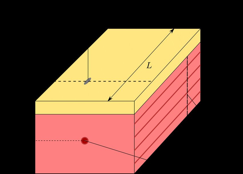
2                                                                                                    Thomas Klotz et al.

aspects of neuromuscular physiology. In the past, how-        ology. However, this approach could not explain some
ever, it was almost only EMG that has been used to            of their experimental observations. This is mainly due
study neuromuscular physiology (for a review see Mer-         to the oversimplification of the muscle’s anatomy as
letti and Farina (2016)). While EMG can be recorded           well as its physiology. Zuo et al (2020, 2021) followed
either intramuscularly or from the body surface, from a       a full-field approach, which was originally proposed by
practical point of view, non-invasive measurements are        Woosley et al (1985), to simulate the magnetic field
desirable. Signals obtained from surface EMG, however,        of an isolated axon. Thereby, the muscle fibres and the
exhibit limited spatial resolution, as the volume conduc-     extracellular connective tissue are modelled as spatially
tive properties of subcutaneous tissues act as low pass       separated regions, whereby the coupling conditions are
filter. This means, a single surface EMG channel records      determined from a pre-computed transmembrane po-
from relatively large tissue volumes making it challeng-      tential. While this approach allows to calculate both
ing to separate and accurately reconstruct the bioelec-       the electrical potential field and the magnetic field in
tromagentic sources. As the magnetic permeability of          a small tissue sample, the computational demands are
biological tissues is close to the magnetic permeability      substantial limiting its use for simulating larger tissue
in free space (Malmivuo et al, 1995, Oschman, 2002),          samples. Further, the decoupling of the transmembrane
MMG has the potential to outperform the spatial res-          potential from the intracellular and extracellular po-
olution of surface EMG. Further, in contrast to EMG,          tential fields is a simplification potentially limiting the
MMG recordings do not rely on sensor-tissue contacts          credibility of the resulting modelling predictions.
and thus are particularly appealing for long term mea-            To enable systematic in silico investigations for both
surements; e. g., prosthesis control via implanted sen-       EMG and MMG signals, we extend our homogenised
sors (Zuo et al, 2020). Although MMG was already first        multi-domain modelling framework (Klotz et al, 2020)
described by Cohen and Givler in 1972, there still exist      to predict both the skeletal-muscle-induced electric and
several challenges that limit its practical use. Most im-     magnetic field. After establishing the model, we first
portantly the amplitude of the magnetic field induced         investigate the hypothesis that for non-invasive record-
by skeletal muscles is very low, i. e., in the range of       ings MMG provides a better spatial selectivity than
pico- to femto-Tesla and, thus, significantly lower than      EMG. Further, we use our model to quantify the contri-
the earth’s magnetic field. This yields high technical de-    butions of different structural components to a muscle
mands for MMG recording systems (Zuo et al, 2020),            induced biomagentic field.
for example, with respect to the sensitivity, the detec-
tion range, the sampling rate, the shielding from mag-
netic noise, the size and portability of the sensor device
                                                              2 Methods
as well as the cost of such recordings. Nevertheless, a
few proof-of-concept studies, e. g. Broser et al (2018,
                                                              2.1 Modelling framework
2021), Llinás et al (2020), Reincke (1993), illustrate its
feasibility for biomedical applications.
                                                              This section presents the modelling framework for in-
    Despite originating from the same phenomenon,             vestigating relations between the biophysical state of
there hardly exist any studies that investigate the           the neuromuscular system and muscle induced bioelec-
biophysical factors affecting MMG or compare MMG              tromagnetic fields. The underlying governing equations
recordings with EMG. Beside experimental studies, sys-        are the quasi-static Maxwell’s equations as presented
temic in silico models can be used to investigate the         in Sect. 2.1.1. As the quasi-static approximation of
factors influencing bioelectromagentic signals and to         Maxwell’s equations allows us to decouple the electric
test hypothesis derived from experimental observations.       field from the magnetic field, we first derive a systemic
Particularly, continuum field models have been success-       multi-scale model to simulate the electro-physiological
fully used for assisting the interpretation of EMG sig-       behaviour of skeletal muscles (Klotz et al, 2020, cf.
nals, e. g., Dimitrova et al (1999), Farina et al (2002,      Sect. 2.1.2) as well as electrically inactive tissue that
2004), Klotz et al (2020), Lowery et al (2002), Mesin         surrounds the respective muscle tissue (cf. Sect. 2.1.3).
(2005), Mesin et al (2006), Mordhorst et al (2015, 2017).     Based on the electric potential field in the region of in-
In contrast, models to simulate magnetic fields induced       terest, the corresponding current densities, and, hence,
by skeletal muscles are still rare. Common to all MMG         the prediction of the magnetic field, can be calculated
models is that they first calculate the current field,        (cf. Sect. 2.1.4). Sect. 2.1.5 provides appropriate bound-
which is then used to obtain the magnetic field. For          ary conditions to guarantee existence and uniqueness
example, Broser et al (2021) used a finite wire model         for the solution of the derived system of partial differ-
to infer from their measurements the underling physi-         ential equations.
Investigating the spatial resolution of EMG and MMG based on a systemic multi-scale model 3
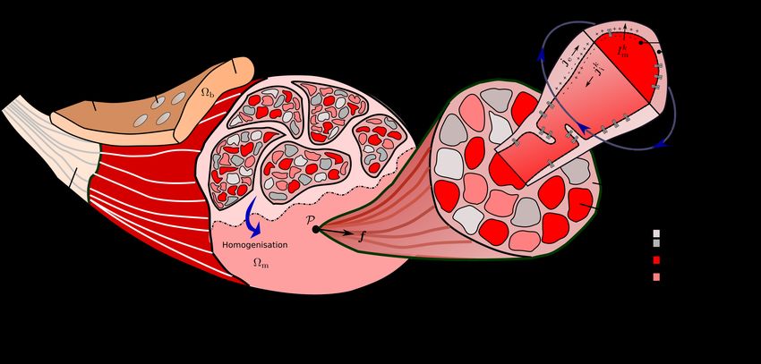
Fig. 1 Schematic drawing illustrating the concept of the proposed multi-scale model. On the macroscale, the heterogeneous
muscle structure is smeared and represented by an idealised and continuous multi-domain material. To couple the different
domains, the multi-scale model still captures the most important features of the original structure. That is, the motor unit
composition on the mesoscale and the interaction of one representative muscle fibre per motor unit and the extracellular space
through the muscle fibre membrane on the microscale. Note that for the muscle fibres each colour represents a different motor
unit. Based on those key properties, the continuous field approach predicts experimental measurable fields such as the trans-
k
membrane potentials Vm , the extracellular potential φe or the magnetic B field. Particularly non-invasive surface recordings,
which are schematically illustrated by the sensors on the surface, of the electrical potential field, i. e., via electromyography
(EMG), or the magnetic field, i. e., via magnetomyography (MMG), are preferable as they yield minimal discomfort for a
subject.
2.1.1 Governing equations law (Eqn. (1d)) yields the conservation of charges, i. e.,
In classical physics, the evolution of the electric and
magnetic field is described by Maxwell’s equations. div j = 0 . (2)
Since changes to the muscle induced electric and mag-
netic field are relatively slow, i. e., the characteristic Exploiting the fact that the electrical field intensity,
time scale is in the range of milliseconds, the electro- E, is a conservative vector field and, thus, can be de-
static and the magnetostatic approximation holds for rived from a scalar potential, i. e. E = − grad φ with
modelling the EMG and MMG signal. The differential grad(·) being the gradient operator, reduces the num-
form of the quasi-static Maxwell’s equations is given by, ber of state variables. Further, introducing the mag-
e. g., Griffiths (2013), netic vector potential A such that
v B = rot A (3)
div E = , (Gauss’s law) (1a)
ε0
div B = 0, (Gauss’s law for magnetism) (1b) and calibrating it by Coulomb gauge, i. e., div A = 0,
we obtain the quasi-static Maxwell’s equations in po-
curl E = 0, (Faraday’s law) (1c)
tential form:
curl B = µ0 j. (Ampère’s law) (1d)
v
div(grad φ) = − , (4a)
Therein, div(·) denotes the divergence operator, curl(·) ε0
denotes the curl operator, E is the electrical field inten- div(grad A) = −µ0 j . (4b)
sity, v is the electrical charge density, ε0 is the vacuum
permittivity, B is the magnetic field (sometimes also Next, we will introduce suitable modelling assumptions
referred to as magnetic flux density), µ0 is the vacuum reflecting the electro-physiological properties of skeletal
permeability and j is the total electrical current den- muscle tissue. Thereby note that for skeletal muscles,
sity. Further, applying the div-curl identity to Ampère’s bound currents are assumed to be negligible and thus4 Thomas Klotz et al.
the total current density j is equal to the ”free” cur- transmembrane current density, i. e., resolving the (mi-
rent density (which is also sometimes called conductive croscale) behaviour of the muscle fibre membranes. The
current density). conservation of charges holds for each skeletal mus-
cle material point if the current density outward vol-
2.1.2 Modelling the electrical behaviour of skeletal ume flux from the extracellular domain is equal to the
muscles weighted sum of the transmembrane current densities,
i. e.,
The electrical behaviour of skeletal muscles is simulated
based on the multi-domain model presented in Klotz N
X
et al (2020) and is briefly summarised here. Skeletal div j e = − frk Akm Im
k
, in Ωm , (7)
muscle tissue consists of muscle fibres associated with k=1
different motor units and extracellular connective tis-
sue (cf. Fig. 1). The multi-domain model resolves this where j e is the extracellular current density. Further,
tissue heterogeneity by assuming that there coexist at frk is a (mesoscale) parameter, reflecting the motor unit
each skeletal muscle material point P ∈ Ωm an ex- composition at each skeletal muscle material point, i. e.
tracellular space and N intracellular spaces, with N the volume fraction of all muscle fibres belonging to mo-
denoting the number of motor units. Given this ho- tor unit k (∀k ∈ MMU ) divided by the volume fraction
mogenized tissue representation, an electrical poten- of all muscle fibres.
tial is introduced for each domain, i. e., φe and φki ,
The (conductive) current densities are related to the
∀ k ∈ MMU := {1, 2, ..., N }, where the subscripts (·)e
electrical potential fields via Ohm’s law, i. e.,
and (·)i denote extracellular and intracellular quanti-
ties, respectively. Further, a transmembrane potential
Vmk is introduced for each motor unit, i. e., j e = −σ e grad φe ,
(8)
j ki = −σ ki grad φki , ∀ k ∈ MMU ,
Vmk = φki − φe , ∀ k ∈ MMU . (5)
The domains are electrically coupled, which is mod- where σ e and σ ki denote the extracellular conductiv-
elled by taking into account the most important fea- ity tensor and the intracellular conductivity tensors,
tures of skeletal muscles mesostructure and microstruc- respectively.
ture as well as the dynamics of the muscle fibre mem- k
Finally, the transmembrane current densities, Im
branes. Thus, the multi-domain model can be classified
(∀k ∈ MMU ), are calculated from an electrical circuit
as a multi-scale model.
model (Hodgkin and Huxley, 1952, Keener and Sneyd,
The conservation of charges, i. e., Eqn.(2), requires
2009) of the muscle fibre membranes via Kirhhoff’s cur-
that all outward volume fluxes of the current densities
rent law, i. e.,
from all domains are balanced at each skeletal muscle
material point. For skeletal muscles it can be assumed
k k k k
that ions can only be exchanged between an intracel- Im = Cm V̇m + Iion (y k , Vmk , Istim
k
),
lular domain and the extracellular space. There exist ẏ k = g k (y k , Vmk ) ,
no current fluxes between the different intracellular do- (9)
mains. As the muscle fibres of the same motor unit y k0 = y k (t = 0) ,
k
are assumed to show similar biophysical properties, the Vm,0 = Vmk (t = 0) .
coupling between an intracellular space k and the extra-
cellular space is modelled by considering the interaction k
of one representative muscle fibre per motor unit with Therein, Cm is the membrane capacitance per unit
the extracellular space. Therefore, the current density area of a muscle fibre belonging to motor unit k,
k
outward volume flux of an intracellular domain is Iion (y k (t), Vmk , Istim
k
) is the total ohmic current density
through a membrane patch associated with MU k and
k
div j ki = Akm Im
k
, k ∈ MMU , in Ωm , (6) Istim is an external stimulus that is used to describe the
motor nerve stimuli of motor unit k at the neuromuscu-
where j ki is the current density of motor unit k in lar junctions. Further, y k is a vector of additional state
a representative fibre-matrix cylinder. Further, Akm is variables, e. g., describing the probability of ion chan-
the surface-to-volume ratio of a muscle fibre belong- nels to be open or closed and g k (y k , Vmk ) is a vector-
ing to motor unit k, i. e., representing the geometry valued function representing the evolution equation for
k
of the muscle fibres on the microscale, and Im is the the membrane state vector y k .Investigating the spatial resolution of EMG and MMG based on a systemic multi-scale model 5
Combing Eqns. (5)-(9) yields for each P ∈ Ωm the each domain independently (cf. Eqn. (8)). To derive the
following system of coupled differential equations: right-hand side of Ampère’s law from domain-specific
current densities, we consider its integral form, i. e.,
0 = div [σ e grad φe ]
N
X
I
frk div σ ki grad Vmk + φe , B dl = µ0 Ienc . (12)
+ (10a)
C
k=1
∂Vmk 1
div σ ki grad Vmk φe
= k k
Therein C is an arbitrary closed curve, Ienc is the total
∂t Cm Am current crossing C and dl is an infinitesimal line ele-
− Akm Iion
k
(y k , Vmk ) , ∀ k ∈ MMU , (10b) ment. Eqn. 12 shows that the currents of the individual
domains simply add up linearly. Since the current den-
ẏ k k
= g (y k
, Vmk ) , ∀ k ∈ MMU . (10c) sities are given with respect to a representative fibre-
Further details can be found in Klotz et al (2020). matrix cylinder, the contributions of the intracellular
current densities j ki (∀k ∈ MMU ) need to be weighted
by the (mesoscale) motor unit density factor frk . Ac-
2.1.3 Modelling the electrical behaviour of inactive
cordingly, the magnetic vector potential for every ma-
tissues
terial point within the muscle region P ∈ Ωm is
Skeletal muscles are surrounded by electrically inactive
N
tissues, e. g., connective tissues, fat or skin. Electrically X
div(grad Am ) = µ0 j e + frk j ki ,
inactive tissues have a strong influence on the electrical
k=1
potential on the body surface. From a modelling point
of view, inactive tissue is a volume conductor free of cur- ⇔ div(grad Am ) = −µ0 σ e grad φe (13)
rent sources, cf., e. g., Mesin (2013), Pullan et al (2005) N
X
or Klotz et al (2020), yielding a generalised Laplace + frk σ ki grad(Vmk + φe ) .
equation for each material point within the body re- k=1
gion P ∈ Ωb , i. e.,
Note, the potential formulation is chosen as this
div [σ b grad φb ] = 0 , in Ωb , (11) yields a Poisson-type equation for which various well-
where φb and σ b are the body region’s electrical poten- established numerical solution methods exist. Further,
tial and conductivity tensor, respectively. note that the linearity of the magnetostatic equations
can be exploited to predict the contribution of each do-
main to the experimentally observable magnetic field.
2.1.4 Modelling magnetic fields induced by skeletal The body’s magnetic vector potential, Ab , is calculated
muscle’s electrical activity similarly:
Starting point for predicting the magnetic field is
Ampère’s law, i. e., Eqn. (1d) or Eqn. (4b), which re- div(grad Ab ) = µ0 j b ,
(14)
lates the magnetic field to the total current density. Ex- ⇔ div(grad Ab ) = −µ0 [σ b grad φb ] ,
ploiting that the radius of a muscle fibre is small com-
pared to the characteristic length scale of the macro- where j b is the current density in the body region. In
scopic continuum model and that the muscle fibres are contrast to the electrical field equations, the magnetic
(approximately) of cylindrical shape leads to the as- field equations also need to consider the air surround-
sumption that the contributions of the transmembrane ing the body. Since air can be assumed to be free of
currents to the macroscopic magnetic field cancel each electrical currents, it is modelled by
other out. Further, assuming that for skeletal muscle
tissue the magnetic susceptibility is approximately zero
div(grad Af ) = 0 , in Ωf , (15)
and that, within the limits of the qausi-static approx-
imation, polarisation currents are negligible (cf. e.g.,
Malmivuo et al (1995)), then the overall current den- where Af is the magnetic vector potential within the
sity is fully determined by the conductive current densi- surrounding space Ωf .
ties. The latter is related to the electrical potential field Finally, the experimentally measurable magnetic
via Ohm’s law, and thus, for the homogenised multi- field B can be calculated straight forwardly from
domain model the current density can be calculated for Eqn.(3).6 Thomas Klotz et al.
2.1.5 Boundary conditions Dirichlet boundary conditions are applied to all in-
finitely distant points Γ∞ , i. e.,
Suitable boundary conditions are required to solve the
partial differential equations presented in the previ- A = 0 , on Γ∞ . (21)
ous sections. Recalling that muscle fibres are electri-
It can be shown that the magnetic vector potential is
cally insulated by their membranes, it is assumed that
continuous at the interface between two media (cf. e. g.,
no charges can leave the intracellular domains at their
Griffiths (2013)). This is modelled by
boundary. This is modelled by applying zero Neumann
boundary conditions to the intracellular potential, i. e., Am = Ab , on Γm ∩ Γb , (22a)
Am = Af , on Γm \ Γb , (22b)
σ ki grad φki · nm = 0 ,
on Γm , Ab = Af , on Γout
b . (22c)
⇔ σ ki grad Vmk · nm
(16)
Further, for biological tissues, surface currents are as-
= − σ ki grad φe · nm ,
on Γm , sumed to be negligible (i. e., they only exhibit vol-
ume conduction). Accordingly, the fluxes of the mag-
where ”·” denotes the scalar product and nm is a unit
netic vector potential across any boundary are balanced
outward normal vector at the muscle surface Γm (cf.
(Griffiths, 2013), i. e.,
Fig. 2).
Further, it is assumed that no charges can leave the grad Ab − grad Am · nm = 0 , on Γm ∩ Γb , (23a)
body, yielding zero Neumann boundary conditions for
grad Af − grad Am · nm = 0 , on Γm \ Γb , (23b)
the electrical potential in the body region, i. e.,
grad Af − grad Ab · nout = 0 , on Γout
b b . (23c)
[σ b grad φb ] · nout
b = 0, on Γout
b . (17)
Therein, nout
b denotes a unit outward normal vector of
Γout
the body surface Γout
b (cf. Fig. 2). In case that the outer
b
Γm ∩ Γb
surface of the simulated region is the skeletal muscle tis-
Ωf
sue’s boundary (or part thereof), the same assumption
Ωm nm Ωb nout ... Γ∞
holds – however with zero Neumann boundary condi- nb b
tions for the extracellular potential, i. e.,
[σ e grad φe ] · nm = 0 , on Γm \ Γb . (18) Γm \ Γb
Fig. 2 Schematic illustration of an arbitrary geometrical rep-
While these are idealised cases typically not reflecting resentation of muscle tissue Ωm , the body region Ωb , the sur-
exact in vivo conditions, it should be noted that this rounding space Ωf , and its respective interfaces. Thereby, Γm
boundary condition is still useful as most in silico exper- denotes the muscle boundary with unit outward normal vec-
iments are restricted to a particular region of interest. tor nm , Γout
b is the body surface with unit outward normal
vector nout
b , Γb is an inner boundary of the body region with
Finally, it is assumed that at the muscle-body inter- unit outward normal vector nb and Γ∞ refers to the set of
face, the extracellular potential φe , and the electrical infinitely distant points.
potential of the body region φb are continuous, i. e.,
φe = φb , on Γm ∩ Γb . (19)
Further, the current flux between the extracellular 2.2 In silico experiments
space and the body region is balanced, yielding
The main aim of this work is to employ the previously
described modelling framework to investigate the spa-
σ e grad φe − σ b grad φb · nm = 0 , on Γm ∩ Γb . (20)
tial resolution of non-invasive EMG and MMG. This is
Note electrical potential fields are not unique, i. e., they achieved by simulating a muscle with a layer of subcu-
can be shifted by an arbitrary scalar value. To make the taneous fat on top and which is variable in thickness.
solution unique, one can mimic/simulate a grounding We exclude the influence of the geometry by focusing on
electrode at a boundary location. a cube-shaped (half) muscle sample with edge lengths
For the magnetic vector potential it can be assumed L = 4.0 cm, W = 1.5 cm and H = 2.0 cm (cf. Fig. 3).
that far away from the muscle, i. e., the bioelectromag- The muscle fibres are aligned with the longest edge, i. e.,
k
netic sources, the magnetic field vanishes. Thus zero denoted as the xl -direction. The spatial selectivity isInvestigating the spatial resolution of EMG and MMG based on a systemic multi-scale model 7
Parameter Symbol Value (slow to fast) Reference
Longitudinal intracellular conductivity σil 8.93 mS cm−1 Bryant (1969)
Transversal intracellular conductivity σit 0.0 mS cm−1 cf. Klotz et al (2020)
Longitudinal extracellular conductivity σel 6.7 mS cm−1 Rush et al (1963)
Transversal extracellular conductivity σet 3.35 mS cm−1 cf. Klotz et al (2020)
Fat conductivity σb 0.4 mS cm−1 Rush et al (1963)
Membrane capacitance Cmk
1 µF cm−2 Hodgkin and Huxley (1952)
Surface-to-volume ratio Akm 500 cm−1 cf. Klotz et al (2020)
Motor unit density frk Variable
Magnetic permeability µ0
Table 1 Summary of model parameters.
addressed by a set of in silico experiments, whereby the
muscle fibres, i. e., the intracellular domains, are selec-
tively stimulated at different depths, i. e., at d = 0.3 cm,
0.5 cm, 0.7 cm, 0.9 cm and 1.1 cm. To do so, we first sub-
divide the muscle into two motor units. All recruited
fibres are grouped into the first motor unit (MU1). The
territory of MU1 is defined by all points at the cross
k
sectional coordinates xt = 0.75 cm and x⊥ t = 2 cm − d.
The territory of the second motor unit (MU2) contains
all points that are not included in the territory of MU1.
Hence, for both motor units, we choose frk (i = 1, 2).
To stimulate the fibres, a single current pulse with am-
plitude 700 mA cm−2 and length 0.1 ms is applied to
the muscle fibre membranes of MU1 at their neuro- Fig. 3 Schematic drawing illustrating the simulated tissue
k k geometry, whereby muscle and fat tissue are coloured in red
muscular junctions, i. e., at xl = 1 cm, xt = 0.75 cm
⊥ and yellow, respectively. The muscle fibres are aligned with
and xt = 2 cm − d. In order to compare measurements k
the xl -direction.
from the muscle surface and the body surface, the simu-
lations are conducted for an isolated muscle (i. e., dfat =
0.0 cm) as well as with adipose tissue layers with thick- and magnetic field. We assume an idealised recording
ness dfat = 0.2 cm and 0.4 cm on top of that muscle. system that does not affect the physical fields. It mea-
All other model parameters are summarised in Table 1. sures at a selected discrete location (i. e. channel) the
Based on these parameters, the intracellular conductiv- extracellular potential (or the body potential) and all
ity tensors are calculated by σ ki = σil f ⊗f (∀k ∈ MMU ), three components of the magnetic field yielding a mea-
where f is a unit vector aligned with the muscle fibre di- surement vector
rection. Accordingly, the extracellular conductivity ten- ( k k
sor is given by σ e = σel f ⊗ f + σet (I − f ⊗ f ) with I [φe , Bl , Bt , Bt⊥ ]T , x ∈ Ωm ,
m(x, t) = k k (24)
being the second-order identity tensor. To simulate the [φb , Bl , Bt , Bt⊥ ]T , x ∈ Ωb .
behaviour of the muscle fibre membranes, we appeal to
the model of Hodgkin and Huxley (1952), which was k
Therein Bl is the magnetic field component aligned
imported from the models repository of the Physiome with the muscle fibres (and tangential to the muscle
Project1 (cf. Lloyd et al (2004)). Finally we note that k
surface), Bt is the component of the magnetic field or-
the given model can only be solved numerically and the thogonal to the muscle fibres and tangential to the sur-
applied methods are presented in Appendix A. face, and Bt⊥ is the magnetic field component normal to
the body surface (and orthogonal to the muscle fibres),
cf. Fig. 3. We assume a sampling frequency of 10 000 Hz
2.3 Virtual EMG and MMG recordings and data
for both the synthetic EMG and MMG.
analysis
To quantitatively evaluate the relation between the
amplitude of the signal components and the geometri-
The computational model yields at each time step and
cal configuration, the root-mean-square (RMS) value is
each grid point a prediction for the electrical potential
calculated for the virtual EMG and MMG signals. Fur-
1
https://models.physiomeproject.org/cellml ther, the spectral content of the virtual signals is inves-8 Thomas Klotz et al.
tigated by estimating the power spectral density (PSD). Depth (cm) 0.3 0.5 0.7 0.9 1.1
Both metrics provide insights on the spatial resolution EMG-RMS 1 0.468 0.270 0.177 0.124
of EMG and MMG signals. EMG-MNF 1 0.802 0.714 0.678 0.660
k
MMG-RMS (xl ) 1 0.445 0.184 0.076 0.031
k
MMG-MNF (xl ) 1 0.788 0.699 0.639 0.592
3 Results
k
MMG-RMS (xt ) 1 0.728 0.507 0.3766 0.3171
k
3.1 Single channel recordings at the muscle surface MMG-MNF (xt ) 1 0.715 0.598 0.521 0.444
MMG-RMS (x⊥
t ) 1 0.286 0.101 0.041 0.019
As baseline experiment, the spatial resolution of EMG MMG-MNF (x⊥
t ) 1 0.902 0.858 0.847 0.854
and MMG signals is investigated for an isolated muscle. Table 2 Effect of the depth of the activated muscle fibres on
To do so, the muscle fibres are selectively stimulated in the RMS and the MNF of the surface EMG signal and sur-
different depths within the muscle tissue (cf. Sect. 2.2). face MMG signal. Note that for the virtual MMG recordings
The muscle response is observed from a single chan- each component of the magnetic field is measured individually
and which is indicated by the respective coordinate shown in
nel, which is placed between the innervation zone and brackets. All values are normalised with respect to the values
the boundary of the muscle on its surface (cf. Fig. 3), from the simulation with the lowest depth, i. e., 0.3 cm.
k k
i. e., xl = 2.5 cm and xt = 0.6 cm. The bottom row
of Fig. 4 shows that the amplitude of all components
of measurement vector m (i. e., the extracellular po- muscle’s response is observed from a single channel at
k k
tential φe and three components of the magnetic field xl = 2.5 cm, and xt = 0.6 cm. Fig. 5 depicts that the
B) decreases with increasing activation depth. In de- amplitude of the surface signal strongly depends on the
tail, the decrease in amplitude is most distinct for the thickness of the fat tissue layer for the EMG. The same
k k
surface normal component of the magnetic field, i. e., holds for the xt -component and the xf -component of
for a depth of 1.1 cm the RMS decreases by a factor the MMG. In detail, for the in silico experiments with
of 0.019 if compared to the RMS at d = 0.3 cm (cf. fat tissue layers of 0.2 cm and 0.4 cm, the RMS of the
Table 2). The signal decay is least pronounced for the EMG signal increases by a factor of 1.67 and 2.72 when
magnetic field component tangential to the body sur- compared to the case without fat. For the MMG compo-
face and orthogonal to the muscle fibre direction, i. e., nent aligned with the muscle fibres, the RMS decreases
for a depth of 1.1 cm the RMS decreases by a factor by a factor of 0.80 and 0.61, respectively. As far as the
k
of 0.317 of the RMS at d = 0.3 cm. For the same con- xt -component of the MMG is concerned, the RMS val-
dition the RMS of the EMG decreases by a factor of ues change by a factor of 0.55 (dfat = 0.2 cm) and 0.63
0.124 and the MMG component aligned with the mus- (dfat = 0.4 cm) compared to the respective reference
cle fibres decreases by a factor of 0.031. Further, from RMS value without fat. Thereby, one also observes a
Fig. 4 and Table 2 it can be seen that increasing the notably modulated shape of the surface potential. This
depth of the stimulated fibres causes a left-shift in the is also reflected by a change of the signal’s frequency
mean frequency content of the observed signals. This spectrum. In contrast, the amplitude and the frequency
indicates a spatial low-pass filtering effect of the mus- content of the normal-to-the-body-surface component
cle tissue, of which the surface normal component of the are less affected by the adipose tissue. For the in silico
magnetic field exhibits the lowest modulation. Further, experiment with dfat = 0.4 cm, the RMS value of the
the shift in the mean frequency content is relatively x⊥t -component changes only by a factor of 1.16 com-
k
smaller for the EMG than for the xl -component and pared to the simulation without fat.
k
the xt -component of the MMG.
3.3 The spatial distribution of the amplitude for
3.2 Single channel recordings at the body surface surface signals
To investigate the influence of adipose tissue on non- Further insights on the spatial selectivity of both EMG
invasively observable surface signals, we compare the and MMG signals can be gained, when considering the
computed fields for three cases with variable fat tissue dependency between the sensor position and the bio-
thickness, i. e., 0 cm, 0.2 cm and 0.4 cm. The distance electromagentic signals. To do so, we evaluate the root
between the recording point and the active fibres is mean square (RMS) for all components of the measure-
kept constant. Hence, when a thicker fat tissue layer ment vector m in a line orthogonal to the muscle fibres
is simulated more superficial fibres are stimulated, i. e., and mid way through the innervation zone and the mus-
d = 0.9 cm, 0.7 cm and 0.5 cm, respectively. Again, the cle boundary (cf. Fig. 3). Fig. 6 shows that the spatialInvestigating the spatial resolution of EMG and MMG based on a systemic multi-scale model 9
k
distribution of the signal’s power is fundamentally dif- the xl -component, is completely determined by volume
ferent between the EMG and the MMG-components. currents in the extracellular space and the body region.
For the EMG signal, the amplitude reaches its maxi- The RMS of the extracellular contribution is 0.950 and
k
mal value directly over the active fibres. For the xl - the RMS of the body region contribution is 0.051 (nor-
component and x⊥ t -component of the MMG, the sig- malised with respect to the RMS value of the observable
nal’s amplitude is zero directly over the source. Further, magnetic field). In contrast, the magnetic field compo-
the depth of the active fibre correlates with the distance nents orthogonal to the muscle fibre direction, i. e., the
k
to the maximum. Considering the case without fat, the xt -component and the x⊥ t -component, depend on cur-
k
distance between the zero value of the xl -component rents from all domains. Thereby, the non-recruited mus-
(directly over the source) and the maximal RMS value cle fibres considerably contribute to the experimentally
is 0.2 cm for a fibre depth of 0.3 cm, 0.3 cm for a fibre observable magnetic field; for the presented simulation,
depth of 0.5 cm, and saturates at 0.35 cm for higher fibre the currents in the active and passive muscle fibres have
depths. Similarly, for the x⊥
t -component and in the case opposite directions and thus mutually limit their visi-
without fat, the distance between the maximum RMS bility in the observable magnetic field. In detail, for
k
value and the zero value is 0.2 cm for a fibre depth of the xt -component the domain specific RMS values nor-
0.3 cm, 0.3 cm for a fibre depth of 0.5 cm, 0.4 cm for a malised with respect to the measurable field are 0.999
fibre depth of 0.7 cm, 0.45 cm for a fibre depth of 0.9 cm for the extracellular space, 0.670 for the active intra-
and 0.5 cm for a fibre depth of 1.1 cm. Further, it can cellular domains, 0.357 for the non stimulated intracel-
k
be seen that the RMS distribution of the xt -MMG- lular domains and 0.027 for the body region. Consid-
component strongly depends on the fat tissue layer and ering the normal-to-the-body-surface component, then
does not follow a distinct pattern. When increasing the the active fibres dominate the measurable signal, i. e.,
thickness of the fat tissue layer, for the EMG it can be the RMS normalised with respect to the RMS value
observed that the inter-channel variability gets strongly of the observable magnetic field is 1.485. Further, the
compressed. For example, for a fibre depth of 0.3 cm normalised RMS values are 0.517 for the passive intra-
the coefficient of variation of the RMS values is 63.6 % cellular domains, 0.134 for the extracellular space and
for the case without fat, 43.4 % for dfat = 0.2 cm and 0.002 for the body region.
22.9 % for dfat = 0.4 cm. In contrast, the MMG com-
ponents aligned with the muscle fibres and normal to
the surface better preserve the inter-channel variability. 4 Discussion
Considering the in silico experiment with a fibre depth
of 0.3 cm, the coefficient of variation of the RMS val- Within this work we propose a novel in silico frame-
k
ues for the xl -component is 73.1 % in the case there is work to simulate electro-magnetic fields induced by
no fat, 61.6 % for dfat = 0.2 cm and 58.6 % for dfat = the activity of skeletal muscles. The model is used for
0.4 cm. For the x⊥ t -component the coefficient of varia- the first systematic comparison between the well es-
tion of the RMS values is 49.5 % in the case without fat, tablished EMG measurements, cf. Merletti and Farina
40.2 % for dfat = 0.2 cm and 37.9 % for dfat = 0.4 cm. (2016), and MMG which recently gained attention due
to progress in sensor technology (cf. e.g., Broser et al,
3.4 The contribution of different domains to the 2018, 2021, Llinás et al, 2020, Zuo et al, 2020).
magnetic field
To investigate the origin of the experimentally observ- 4.1 Limitations
able magnetic fields, the MMG recorded on the body
surface is split up into the contribution of the different The presented systemic multi-scale approach integrates
domains. To do so, we exploit the linearity of the mag- the most important features of the microstructure, for
netic field equations, i. e., Eqn. 13 and Eqn. 14. There- example, the shape of the muscle fibres and the electri-
fore, the solution of the overall magnetic field problem cal behaviour of the fibre membranes. It must be noted
can be linearly reconstructed from the individual solu- that the effects of currents in complex microstructural
tions of each right hand term, i. e., the contribution of features such as the T-tubuli system is beyond the scope
each domain / region (cf. Sect. 2.1.4). In Fig. 7 this is of the proposed model. Further, while we use an ide-
exemplary shown for the in silico experiment with a alised cubic muscle geometry to ignore geometric ef-
fat tissue layer of 0.2 cm and active muscle fibres in a fects and illustrate the basic properties of the magnetic
depth of 0.5 cm. It can be observed that the component field induced by active muscles, the MMG is expected
of the magnetic field aligned with the muscle fibres, i. e., to strongly depend on the specific muscle geometry.10 Thomas Klotz et al.
Thereby, it should be noted that the presented contin- a much less pronounced influence of the fat layer. Par-
uum field approach provides a high flexibility to resolve ticularly, the spatial-temporal pattern of the normal-
arbitrary muscle geometries by employing discretiza- to-the-surface component is nearly preserved (cf. Fig. 5
tion schemes such as the finite element method, e.g., and Fig. 6). Thus, we conclude that a careful selection of
Heidlauf et al (2016), Mordhorst et al (2015), Schmid the measured magnetic field component can overcome
et al (2019). Finally, we note that within this work we the limitations given by the poor spatial selectivity of
focused on the physical properties of the bioelectro- surface EMG.
magentic fields. Hence, we considered idealised sensors The potentially most interesting implication of sur-
that can record from a single point in space and mea- face MMG’s increased spatial selectivity is the rela-
surements are unaffected by noise. However, for specific tively higher sparseness of the magnetic interference sig-
applications the specific sensor properties need to be nals. This advocates for the use of non-invasive MMG
considered for comparing EMG and MMG. recordings to decode the neural drive to a muscle using,
e. g. Farina et al (2014), Holobar et al (2010), Nawab
et al (2010), Negro et al (2016) as the impact on the
4.2 The spatial resolution of EMG and MMG interference of the different sources will be less pro-
nounced. Further, it limits the signal’s contamination
The spatial resolution is one of the most extensively dis- with cross-talk. On the other hand, it should be noted
cussed property of EMG. That is, when employing inva- that a higher spatial selectivity also implies that rather
sive intramuscular electrodes, EMG is highly sensitive local properties of the muscle tissue are observed. This,
with respect to the spatial coordinate of the recording if not compensated by a congruous amount of sensors,
point. However, when measured non-invasively from the may compromise the robustness and comparability of
skin EMG has a poor spatial resolution as surrounding measurements as a too pronounced weighting of local
electrically inactive tissues, such as, for example, fat, properties yields the risk to bias the observations. This
act as a spatial low pass filter. Within this work we ad- is a well-known limitation of intramuscular EMG de-
dress the hypothesis that surface MMG can overcome composition (cf. e. g., De Luca et al, 2006, Farina and
the limitations of surface EMG’s spatial selectivity. We Negro, 2012, Farina et al, 2010). Further, it is noted
did so by carrying out an in silico comparison between that a higher spatial selectivity makes measurements
both bioelectric and biomagnetic signals. more susceptible for motion artifacts.
EMG and MMG measure different physical fields
and therefore are not directly comparable. Thus, as a 4.3 The biophysical origin of the measurable magnetic
reference experiment we investigated the spatial prop- field
erties for EMG and MMG signals directly recorded on
the surface of an isolated muscle. When the distance We make use of the systemic modelling framework to
between the recording point and the active muscle fi- deduce the biophysical origin of the magnetic field in-
bres is increased, all MMG components and the EMG duced by muscle activity. An electrical current only can
show a strong decrease in amplitude. Hence, we con- generate a magnetic field circular to the direction of the
clude that for both intramuscular electrical field and current. Accordingly, we showed that the magnetic field
magnetic field recordings the spatial resolution should aligned with the muscle fibres, is fully determined by
be reasonable to observe local events within the tissue. volume currents in the extracellular space / surround-
This, however, changes, if we consider non-invasive sur- ing tissues. In contrast, both magnetic field components
face recordings (which are affected by electrically in- orthogonal to the muscle fibre direction contain contri-
active tissues such as fat). Our simulations show, as butions from intracellular currents, which are in the
previously reported, e. g., Farina et al (2002), Lowery literature sometimes referred to as primary currents
et al (2002), Roeleveld et al (1997), that the spatial (Malmivuo et al, 1995). However, while the MMG com-
selectivity of the EMG is compromised. We conclude ponent tangential to the body surface and orthogonal to
this from the fact that increasing the thickness of the k
the muscle fibres, i. e., the xt -component, is dominated
adipose tissue causes a strong modulation of the EMG by volume currents, the surface-normal component of
signal’s amplitude (cf. Fig. 5 and Fig. 6). the MMG, i. e., the x⊥ t -component, is dominated by in-
k
Considering the MMG’s xt -component, the effect of tracellular currents.
fat tissue on the surface signal is even more pronounced The observation that the surface-normal component
than for EMG. However, in comparison to EMG, our of the magnetic field strongly reflects intracellular cur-
simulations show that the MMG components normal to rents and is relatively insensitive to the effect of fat,
the surface and aligned with the muscle fibres exhibit yields several potential benefits for the interpretation ofInvestigating the spatial resolution of EMG and MMG based on a systemic multi-scale model 11
experimental data. This can be beneficial when prop- A.1 Solving for the electrical potential fields
erties on the muscle fibre level, for example, membrane
fatigue, should be estimated from MMG data. Further, Given the reaction-diffusion characteristic of Eqn. (10b), a
first-order Godunov-type splitting scheme is applied to yield
when aiming to use inverse modelling and MMG to re-
k,t∗ k,ti
construct the sources of the bioelectromagnetic activ- Vm − Vm 1 k
= − k Iion (y k , Vm k
), (25a)
ity, e. g., Llinás et al (2020), a field component which is ∆t Cm
k,t k,t∗
(nearly) invariant with respect to volume currents can Vm i+1 − Vm 1
div σ k k
= i grad Vm +
reduce the uncertainty associated with the required es- ∆t k Ak
Cm m
timate for the tissue’s conductive properties. We con- + div σ k
i grad φe , (25b)
clude this discussion by noting that the model predicts
a surprisingly big contribution of passive muscle fibres. for each skeletal muscle material point P ∈ Ωm and k ∈
MMU . Therein, a first-order forward finite difference is used
to approximate the temporal derivatives and t∗ denotes an
intermediate time step. Note that the hereby introduced split-
ting error becomes acceptable for sufficiently small time steps.
Herein, we chose as time step ∆t = 0.1 ms. Further, note that
both Eqn. (25a) and Eqn. (25b) are still continuous in space.
This allows us to use specialised solution schemes for the re-
4.4 Conclusion and Outlook active and the diffusive parts of the model.
In detail, Eqn. (25a) together with Eqn. (10c) forms a
system of stiff ordinary differential equations, which is solved
Within this work we propose a systemic multi-scale for the interval [ti , t∗ ] by an improved Euler method and
model to simulate EMG and MMG. We show that a fixed time step of ∆tode = 0.001 ms (cf. Bradley et al
(2018)). Further, the coupled diffusion problem given by given
non-invasive MMG can overcome the limitations of sur- by Eqn. (10a), Eqn. 25b and Eqn. (11), is addressed by
face EMG, in particular with respect to its poor spa- evaluating Eqn. (10a), Eqn. (11) and the right-hand side of
tial selectivity. In the future, we want to use the pre- Eqn. (25b) at t = ti+1 , i. e., employing an implicit Euler
sented modelling framework to investigate the poten- method, whereby the spatial derivatives are approximated
with second-order accurate central finite differences. Accord-
tial of non-invasive MMG to decode the neural drive to ingly, the flux boundary conditions, i. e., Eqn. (16), Eqn. (17),
muscles. Further, given the emerging progress in MMG Eqn. (18) and Eqn. (20), are also evaluated at t = ti+1 ,
sensor technology, the presented systemic simulation while being approximated with second-order accurate for-
framework provides excellent capabilities to assist the ward/backward finite differences. For the spatial discretisa-
tion, we chose equally spaced grid points and a step size
interpretation of experimental data as well as assisting of h = 0.05 cm. This discretisation yields a linear system
the optimisation of MMG sensor arrays. of equations which is solved with matlab’s built-in GMRES
function (Saad and Schultz, 1986). The linear system is pre-
conditioned via an incomplete LU factorisation (crout ver-
sion, drop tolerance: 1e-6) and the following solver options are
applied: an absolute and relative tolerance of 1e-10, restart
after 20 inner iterations and a maximum number of 20 outer
iterations.
A Numerical treatment
A.2 Solving for the magnetic vector potential
The mathematical modelling framework presented in this
work, i. e., Sect. 2.1, can only be solved numerically. The ap- Based on the solution of the multi-domain model, i. e., the
plied methods are outlined in the following. In summary, we electrical potential fields for each time step and each grid
exploit the quasi-static conditions and decouple the electric point of the muscle region and body region, second-order cen-
and the magnetic field (cf. Sect. 2.1.1). Thus, we appeal to tral finite differences are used to obtain estimates for the
a staggered solution scheme where (i) the electric field equa- (first) spatial derivative of the electrical potentials of the
tions are solved for the muscle and body domain (cf. A.1) and right-hand side of Eqn. (13) and Eqn. (14). Further, the
(ii) the magnetic field predictions are based on the previously (second) spatial derivatives given on the left-hand side of
calculated electric potentials (cf. A.2). Therefore, the continu- Eqn. (13) and Eqn. (14) are discretised using second-order
ous domains are represented by a finite number of grid points central finite differences.
and the spatial derivatives are approximated by finite differ- As for the electrical potential fields are concerned, the
ences. The whole model is implemented in MATLAB (The flux boundary conditions of the magnetic vector potential
MathWorks, Inc., Natick, Massachusetts, United States) and in the muscle and body region (cf. Eqn. (23)) are approx-
the corresponding code is hosted on a freely accessible git imated with second-order accurate forward/backward finite
repository2 . differences. The surrounding air is represented by an infinitely
long (virtual) boundary element. Its normal derivative (cf.
Eqn. (23)) is approximated by a first-order forward/backward
finte difference. Recalling that the magnetic vector poten-
2
https://bitbucket.org/klotz t/multi domain fd code tial is zero far away from the bioelectromagentic sources (cf.12 Thomas Klotz et al.
Eqn. (21)), the normal derivative of the magnetic vector po- Farina D, Merletti R, Enoka RM (2014) The extraction of
tential vanishes at the interface between the body and air. neural strategies from the surface emg: an update. Journal
In summary, this discretisation yields a linear system of of Applied Physiology 117(11):1215–1230
equations, which needs to be solved to obtain the magnetic Griffiths DJ (2013) Introduction to electrodynamics; 4th ed.
vector potential at each grid point of the muscle and body Pearson, Boston, MA
region. This linear system is solved with MATLAB’s build Heckman CJ, Enoka RM (2012) Motor Unit. Comprehensive
in ”mldivide” function, as this function can handle multiple Physiology 2:2629–2682
pre-computed right-hand side vectors simultaneously. Finally, Heidlauf T, Klotz T, Altan E, Bleiler C, Siebert T, Rode
the magnetic field B is calculated via Eqn. (3) in a post- C, Röhrle O (2016) A multi-scale continuum model of
processing step. Thereby the (first) spatial derivatives of the skeletal muscle mechanics predicting force enhancement
curl operator are approximated by second-order central finite based on actin-titin interaction. Biomechanics and Model-
differences. ing in Mechanobiology 11(10):1424 – 1437, DOI 10.1007/
s10237-016-0772-7
Hodgkin AL, Huxley AF (1952) A quantitative description of
Acknowledgements This research was funded by the membrane current and its application to conduction and
Deutsche Forschungsgemeinschaft (DFG, German Research excitation in nerve. The Journal of Physiology 117(4):500–
Foundation) under Germany’s Excellence Strategy EXC 2075 544, DOI 10.1113/jphysiol.1952.sp004764
390740016. Holobar A, Minetto MA, Botter A, Negro F, Farina D (2010)
Experimental analysis of accuracy in the identification of
motor unit spike trains from high-density surface emg.
IEEE Transactions on Neural Systems and Rehabilitation
Engineering 18(3):221–229
References
Keener J, Sneyd J (2009) Mathematical Physiology II: Cellu-
lar Physiology, vol 2, 2nd edn. Springer
Bradley CP, Emamy N, Ertl T, Göddeke D, Hessenthaler A, Klotz T, Gizzi L, Yavuz U, Röhrle O (2020) Modelling
Klotz T, Krämer A, Krone M, Maier B, Mehl M, Rau T, the electrical activity of skeletal muscle tissue using a
Röhrle O (2018) Enabling detailed, biophysics-based skele- multi-domain approach. Biomechanics and modeling in
tal muscle models on hpc systems. Frontiers in Physiology mechanobiology 19(1):335–349
9:816, DOI 10.3389/fphys.2018.00816 Llinás RR, Ustinin M, Rykunov S, Walton KD, Rabello GM,
Broser PJ, Knappe S, Kajal DS, Noury N, Alem O, Shah Garcia J, Boyko A, Sychev V (2020) Noninvasive muscle
V, Braun C (2018) Optically pumped magnetometers for activity imaging using magnetography. Proceedings of the
magneto-myography to study the innervation of the hand. National Academy of Sciences 117(9):4942–4947
IEEE Transactions on Neural Systems and Rehabilitation Lloyd CM, Halstead MD, Nielsen PF (2004) Cellml: its fu-
Engineering 26(11):2226–2230 ture, present and past. Progress in Biophysics and Molecu-
Broser PJ, Middelmann T, Sometti D, Braun C (2021) Opti- lar Biology 85(2):433 – 450, DOI https://doi.org/10.1016/
cally pumped magnetometers disclose magnetic field com- j.pbiomolbio.2004.01.004, modelling Cellular and Tissue
ponents of the muscular action potential. Journal of Elec- Function
tromyography and Kinesiology 56:102,490 Lowery MM, Stoykov NS, Taflove A, Kuiken TA (2002)
Bryant SH (1969) Cable properties of external intercostal A Multiple-Layer Finite-Element Model of the Surface
muscle fibres from myotonic and nonmyotonic goats. The EMG Signal. IEEE Transactions on Biomedical Engineer-
Journal of Physiology 204:539 – 550, DOI 10.1113/jphysiol. ing 49(5):446–454, DOI 10.1109/10.995683
1969.sp008930 MacIntosh R B, Gardiner F P, McComas J A (2006) Skeletal
Cohen D, Givler E (1972) Magnetomyography: Magnetic Muscle: Form and Function, 2nd edn. Human Kinetics
fields around the human body produced by skeletal mus- Malmivuo J, Plonsey R, et al (1995) Bioelectromagnetism:
cles. Applied Physics Letters 21(3):114–116 principles and applications of bioelectric and biomagnetic
De Luca CJ, Adam A, Wotiz R, Gilmore LD, Nawab SH fields. Oxford University Press, USA
(2006) Decomposition of surface emg signals. Journal of Merletti R, Farina D (2016) Surface electromyography: phys-
neurophysiology 96(3):1646–1657 iology, engineering, and applications. John Wiley & Sons
Dimitrova NA, Dimitrov AG, Dimitrov GV (1999) Cal- Mesin L (2005) Analytical Generation Model Of Surface Elec-
culation of extracellular potentials produced by an in- tromyogram For Multi-layer Volume Conductors. Mod-
clined muscle fibre at a rectangular plate electrode. Med- elling in Medicine and Biology VI, WIT 8:95–110, DOI
ical Engineering & Physics 21:583–588, DOI 10.1016/ 10.2495/BIO050101
S1350-4533(99)00087-9 Mesin L (2013) Volume conductor models in surface elec-
Farina D, Negro F (2012) Accessing the neural drive to muscle tromyography: Computational techniques. Computers in
and translation to neurorehabilitation technologies. IEEE Biology and Medicine 43(7):942 – 952, DOI https://doi.
Reviews in biomedical engineering 5:3–14 org/10.1016/j.compbiomed.2013.02.002
Farina D, Cescon C, Merletti R (2002) Influence of anatom- Mesin L, Joubert M, Hanekom T, Merletti R, Farina D (2006)
ical, physical, and detection-system parameters on surface A Finite Element Model for Describing the Effect of Mus-
emg. Biological cybernetics 86(6):445–456 cle Shortening on Surface EMG. IEEE Transactions on
Farina D, Mesin L, Martina S (2004) Advances in surface Biomedical Engineering 53:693–600, DOI 10.1109/TBME.
electromyographic signal simulation with analytical and 2006.870256
numerical descriptions of the volume conductor. Medical Mordhorst M, Heidlauf T, Röhrle O (2015) Predicting elec-
& Biological Engineering & Computing 42:467–476, DOI tromyographic signals under realistic conditions using a
10.1007/BF02350987 multiscale chemo-electro-mechanical finite element model.
Farina D, Holobar A, Merletti R, Enoka RM (2010) Decoding Interface Focus 5(2):1–11, DOI 10.1098/rsfs.2014.0076
the neural drive to muscles from the surface electromyo-
gram. Clinical neurophysiology 121(10):1616–1623Investigating the spatial resolution of EMG and MMG based on a systemic multi-scale model 13 Mordhorst M, Strecker T, Wirtz D, Heidlauf T, Röhrle O (2017) POD-DEIM reduction of computational EMG mod- els. Journal of Computational Science 19:86–96, DOI 10.1016/j.jocs.2017.01.009 Nawab SH, Chang SS, De Luca CJ (2010) High-yield decom- position of surface emg signals. Clinical neurophysiology 121(10):1602–1615 Negro F, Muceli S, Castronovo AM, Holobar A, Farina D (2016) Multi-channel intramuscular and surface emg de- composition by convolutive blind source separation. Jour- nal of neural engineering 13(2):026,027 Oschman JL (2002) Clinical aspects of biological fields: an in- troduction for health care professionals. Journal of Body- work and Movement Therapies 6(2):117–125 Pullan AJ, Buist ML, Cheng LK (2005) Mathematically Mod- elling the Electrical Activity of the Heart: From Cell to Body Surface and Back Again. World Scientific Publishing Company, Singapore, DOI 10.1142/5859 Reincke M (1993) Magnetomyographie mit dem squid - magnetomyography with the squid. Biomedical Engineer- ing – Biomedizinische Technik 38(11):276–281, DOI doi: 10.1515/bmte.1993.38.11.276, URL https://doi.org/10. 1515/bmte.1993.38.11.276 Roeleveld K, Blok J, Stegeman D, Van Oosterom A (1997) Volume conduction models for surface emg; confrontation with measurements. Journal of Electromyography and Ki- nesiology 7(4):221–232 Röhrle O, Yavuz U, Klotz T, Negro F, Heidlauf T (2019) Mul- tiscale modelling of the neuromuscular system: coupling neurophysiology and skeletal muscle mechanics. Wiley In- terdisciplinary Reviews: Systems Biology and Medicine Rush S, Abildskov J, McFee R (1963) Resistivity of body tissues at low frequencies. Circulation research 12(1):40– 50 Saad Y, Schultz MH (1986) Gmres: A generalized minimal residual algorithm for solving nonsymmetric linear sys- tems. SIAM Journal on Scientific and Statistical Comput- ing 7(3):856–869, DOI 10.1137/0907058 Schmid L, Klotz T, Siebert T, Röhrle O (2019) Character- ization of electromechanical delay based on a biophysical multi-scale skeletal muscle model. Frontiers in Physiology 10(1270):1 – 13, DOI 10.3389/fphys.2019.01270 Woosley JK, Roth BJ, Wikswo Jr JP (1985) The magnetic field of a single axon: A volume conductor model. Mathe- matical Biosciences 76(1):1–36 Zuo S, Heidari H, Farina D, Nazarpour K (2020) Miniatur- ized magnetic sensors for implantable magnetomyography. Advanced Materials Technologies 5(6):2000,185 Zuo S, Nazarpour K, Farina D, Broser P, Heidari H (2021) Modelling and analysis of magnetic fields from skeletal muscle for valuable physiological measurements. arXiv preprint arXiv:210402036
You can also read