Learning differential module networks across multiple experimental conditions
←
→
Page content transcription
If your browser does not render page correctly, please read the page content below
Learning differential module networks across
                                            multiple experimental conditions

                                            Pau Erola, Eric Bonnet and Tom Michoel
arXiv:1711.08927v2 [q-bio.QM] 12 Feb 2018

                                            Abstract Module network inference is a statistical method to reconstruct gene reg-
                                            ulatory networks, which uses probabilistic graphical models to learn modules of
                                            coregulated genes and their upstream regulatory programs from genome-wide gene
                                            expression and other omics data. Here we review the basic theory of module net-
                                            work inference, present protocols for common gene regulatory network reconstruc-
                                            tion scenarios based on the Lemon-Tree software, and show, using human gene
                                            expression data, how the software can also be applied to learn differential module
                                            networks across multiple experimental conditions.

                                            Key words: gene regulatory network inference, module networks, differential net-
                                            works, Bayesian analysis

                                            1 Introduction

                                            Complex systems composed of a large number of interacting components often dis-
                                            play a high level of modularity, where independently functioning units can be ob-
                                            served at multiple organizational scales [1]. In biology, a module is viewed as a
                                            discrete entity composed of many types of molecules and whose function is sepa-

                                            Pau Erola
                                            Division of Genetics and Genomics, The Roslin Institute, The University of Edinburgh, Midlothian
                                            EH25 9RG, Scotland, United Kingdom
                                            Eric Bonnet
                                            Centre National de Recherche en Génomique Humaine, Institut de Biologie François Jacob, Di-
                                            rection de la Recherche Fondamentale, CEA, Evry, France
                                            Tom Michoel
                                            Division of Genetics and Genomics, The Roslin Institute, The University of Edinburgh, Midlothian
                                            EH25 9RG, Scotland, United Kingdom. Correspondence to e-mail: Tom.Michoel@roslin.
                                            ed.ac.uk

                                                                                                                                          1
2 Pau Erola, Eric Bonnet and Tom Michoel
rable from that of other modules [2]. The principle of modularity plays an essen-
tial role in understanding the structure, function and evolution of gene regulatory,
metabolic, signaling and protein interaction networks [3]. It is therefore not surpris-
ing that functional modules also manifest themselves in genome-wide data. Indeed,
from the very first studies examining genome-wide gene expression levels in yeast,
it has been evident that clusters of coexpressed genes, i.e. sharing the same expres-
sion profile over time or across different experimental perturbations, reveal impor-
tant information about the underlying biological processes [4, 5]. Module network
inference takes this principle one step further, and aims to infer simultaneously co-
expression modules and their upstream regulators [6, 7]. From a statistical perspec-
tive, modularity allows to reduce the number of model parameters that need to be
determined, because it is assumed that genes belonging to the same module share
the same regulatory program, and therefore allows to learn more complex models,
in particular non-linear probabilistic graphical models [8], than would otherwise be
possible.
While module networks were originally introduced to infer gene regulatory net-
works from gene expression data alone [6], the method has meanwhile been ex-
tended to also include expression quantitative trait loci data [9, 10], regulatory prior
data [11], microRNA expression data [12], clinical data [13], copy number variation
data [14, 15] or protein interaction networks [16]. Furthermore, the method can be
combined with gene-based network inference methods [17, 18]. Finally, the mod-
ule network method has been applied in numerous biological, biotechnological and
biomedical studies [19–29].
An area of interest that has received comparatively limited attention to date con-
cerns the inference of differential module networks. Differential networks extend
the concept of differential expression, and are used to model how coexpression, reg-
ulatory or protein-protein interaction networks differ between two or more experi-
mental conditions, cell or tissue types, or disease states [30,31]. Existing differential
network inference methods are mainly based on pairwise approaches, either by test-
ing for significant differences between correlation values in different conditions,
or by estimating a joint graph from multiple data sets simultaneously using penal-
ized likelihood approaches [32–35]. The inference of differential module networks
is more challenging, because it requires a matching or comparable set of modules
across the conditions of interest. A related problem has been addressed in a study of
the evolutionary history of transcriptional modules in a complex phylogeny, using
an algorithm that maps modules across species and allows to compare their gene
assignments [36].
In this chapter, we review the theoretical principles behind module network in-
ference, explain practical protocols for learning module networks using the Lemon-
Tree software [15], and show in a concrete application on human gene expression
data how the software can also be used to infer differential module networks using
a similar principle as in [36].Learning differential module networks across multiple experimental conditions 3
2 Module network inference: theory and algorithms
2.1 The module network model
Module networks are probabilistic graphical models [7, 8] where each gene gi ,
i ∈ {1, . . . , G}, is represented by a random variable Xi taking continuous values.
In a standard probabilistic graphical model or Bayesian network, it is assumed that
the distribution of Xi depends on the expression level of a set of regulators Pi (the
“parents” of gene i). If the causal graph formed by drawing directed edges from
parents to their targets is acyclic, then the joint probability distribution for the ex-
pression levels of all genes can be written as a product of conditional distributions,
G
p(x1 , . . . , xG ) = ∏ p xi | {x j : j ∈ Pi } .
(1)
i=1
In data integration problems, we are often interested in explaining patterns in one
data type (e.g. gene expression) by regulatory variables in another data type (e.g.
transcription factor binding sites, single nucleotide or copy number variations, etc.).
In this case, the causal graph is bipartite, and the acyclicity constraint is satisfied
automatically.
In a module network, we assume that genes are partitioned into modules, such
that genes in the same module share the same parameters in the distribution function
(1). Hence a module network is defined by a partition of {1, . . . , G} into K modules
Ak , a collection of parent genes Pk for each module k, and a joint probability dis-
tribution
K
p(x1 , . . . , xG ) = ∏ ∏ p xi | {x j : j ∈ Pk } .
(2)
k=1 i∈Ak
In a module network, only one conditional distribution needs to be parameterized
per module, and hence it is clear that if K
G, the number of model parameters
in eq. (2) is much smaller than in eq. (1). Moreover, data from genes belonging to
the same module are effectively pooled, leading to more robust estimates of these
model parameters. This is the main benefit of the module network model.
In principle, any type of conditional distribution can be used in eq. (2). For in-
stance, in a linear Gaussian framework [8], one would assume that each gene is
normally distributed around a linear combination of the parent expression levels.
However, the pooling of genes into modules allows for more complex, non-linear
models to be fitted. Hence it was proposed that the conditional distribution of the ex-
pression level of the genes in module k is normal with mean and standard deviation
depending on the expression values of the parents of the module through a regres-
sion tree (the “regulatory program” of the module) [6] (Figure 1). The tests on the
internal nodes of the regression tree are usually defined to be of the form x ≥ v or
not, for a split value v, where x is the expression value of the parent associated to
the node.4 Pau Erola, Eric Bonnet and Tom Michoel
Hap4 targets in Respiratory
Yeastract database genes
Fig. 1 Example of a module and regulatory decision tree inferred from yeast data, with Hap4 as-
signed as a top regulator. Genes known to be regulated by Hap4 in YEASTRACT are marked in
blue and those involved in respiration are marked in orange. Reused from Joshi et al., Module net-
works revisited: computational assessment and prioritization of model predictions, Bioinformatics,
2009, 25(4):490–496 [37], by permission of Oxford University Press.
Given a module network specification M , consisting of gene module assign-
ments, regulatory decision trees, and normal distribution parameters at the leaf
nodes, the probability density of observing an expression data matrix X = (xim ) ∈
RG×N for G genes in N samples is given by
N K K Lk
P(X | M ) = p xim | {x jm : j ∈ Pk } = ∏ ∏
∏∏∏ ∏ ∏ p(xim | µ` , σ` ),
m=1 k=1 i∈Ak k=1 `=1 i∈Ak m∈E`
where Lk is the number of leaf nodes of module k’s regression tree, E` denotes the
experiments that end up at leaf ` after traversing the regression tree, and (µ` , σ` ) are
the normal distribution paramaters at leaf `. The Bayesian model score is obtained
by taking the log-marginal probability over the parameters of the normal distribu-
tions at the leaves of the regression trees with a normal-gamma prior:
S = ∑ Sk = ∑ ∑ Sk (E` ) (3)
k k `
(`) λ0 (`)
Sk (E` ) = − 12 R0 log(2π) + 12 log − logΓ (α0 ) + logΓ (α0 + 12 R0 )
(`)
λ0 + R0
1 (`)
+ α0 log β0 − (α0 + 2 R0 ) log β1
(`)
where Rq are the sufficient statistics at leaf `,Learning differential module networks across multiple experimental conditions 5
(`) q
Rq = ∑ ∑ xi,m , q = 0, 1, 2,
m∈E` i∈Ak
and
(`) (`) (`) 2
1 h (`) (R1 )2 i λ0 R1 − µ0 R0
β1 = β0 + R2 − (`) + (`) (`)
.
2 R 2(λ0 + R )R
0 0 0
Details of this calculation can be found in [38, 39].
2.2 Optimization algorithms
The first optimization strategy proposed to identify high-scoring module networks
was a greedy hill-climbing algorithm [6]. This algorithm starts from an initial as-
signment of genes to coexpression clusters (e.g. using k-means), followed by as-
signing a new regulator to each module by iteratively finding the best (if any) new
split of a current leaf node into two new leaf nodes given the current set of gene-
to-module assignments, and reassigning genes between modules given the current
regression tree, while preserving acyclicity throughout. The decomposition of the
Bayesian score [eq. (3)] as a sum of leaf scores of the different modules allows for
efficient updating after every regulator addition or gene reassignment.
An improvement to this algorithm was found, based on the observation that the
Bayesian score depends only on the assignment of samples to leaf nodes, and not
on the actual regulators or tree structure that induce this assignment [39]. Hence, a
decoupled greedy hill-climbing algorithm was developed, where first the Bayesian
score is optimized by two-way clustering of genes into modules and samples into
leaves for each module, and then a regression tree is found for the converged set of
modules by hierarchically merging the leave nodes and finding the best regulator
to explain the split below the current merge. This algorithm achieved comparable
score values as the original one, while being considerably faster [39].
Further analysis of the greedy two-way clustering algorithm revealed the exis-
tence of multiple local optima, in particular for moderate to large data sets (∼1000
genes or more), where considerably different module assignments result in near-
identical scores. To address this issue, a Gibbs sampler method was developed,
based on the Chinese restaurant process [40], for sampling from the posterior distri-
bution of two-way gene/sample clustering solutions [41]. By sampling an ensemble
of multiple, equally probable solutions, and extracting a core set of ‘tight clusters’
(groups of genes which consistenly cluster together), gene modules are identified
that are more robust to fluctuations in the data and have higher functional enrich-
ment compared to the greedy clustering strategies [37, 41].
Finally, the Gibbs sampling strategy for module identification was complemented
with a probabilistic algorithm, based on a logistic regression of sample splits on
candidate regulator expression levels, for sampling and ensemble averaging of reg-
ulatory programs, which resulted in more accurate regulator assignments [37].6 Pau Erola, Eric Bonnet and Tom Michoel
3 The Lemon-Tree software suite for module network inference
3.1 Lemon-Tree software package
Lemon-Tree is a software suite implementing all of the algorithms discussed in Sec-
tion 2.2. Lemon-Tree has been benchmarked using large-scale tumor datasets and
shown to compare favorably with other module network inference methods [15].
Its performance has been carefully assessed also in an independent study not in-
volving the software authors [42]. Lemon-Tree is self-contained, with no external
program dependencies, and is entirely coded in the JavaTM programming language.
Users can download a pre-compiled version of the software, or alternatively they can
download and compile the software from the source code, which is available on the
GitHub repository (https://github.com/eb00/lemon-tree). Note that
there is also a complete wiki on the Lemon-Tree GitHub (https://github.
com/eb00/lemon-tree/wiki), with detailed instruction on how to download,
compile, use the software, what are the default parameters and an extended bibliog-
raphy on the topic of module networks.
Lemon-Tree is a command-line software, with no associated graphical user in-
terface at the moment. The different steps for building the module network are done
by launching commands with different input files that will generate different output
files. All the command line examples below are taken from the Lemon-Tree tutorial,
that users are encouraged to download and reproduce by themselves.
The purpose of the Lemon-Tree software package is to create a module network
from different types of ’omics’ data. The end result is a set of gene clusters (co-
expressed genes), and their associated “regulators”. The regulators can be of dif-
ferent types, for instance mRNA expression, copy-number profiles, variants (such
as single nucleotide variants) or even clinical parameter profiles can be used. There
are three fundamental steps or tasks to build a module network with Lemon-Tree
(Figure 2):
• Generate several cluster solutions (”ganesh” task).
• Merge the different cluster solutions using the fuzzy clustering algorithm (”tight clusters”
task).
• Assign regulators to each cluster, producing the module network (”regulators”
task).
3.2 Ganesh task
The goal of this task is to cluster genes from a matrix (rows) using a probabilistic
algorithm (Gibbs sampling) [41]. This step is usually done on the mRNA expres-
sion data only, although some other data type could be used, for instance proteomic
expression profiles. We first select genes having non-flat profiles, by keeping genes
having a standard deviation above a certain value (0.5 is often used as the cutoffLearning differential module networks across multiple experimental conditions 7
Define
a
biological
ques-on,
e.g.
influence
of
copy-‐number
altera8ons
on
co-‐expressed
gene
modules
in
glioblastoma
cancer.
Preprocess
expression
data
matrix
Select
candidate
regulator
types
(sample
and
gene
selec8on,
(gene
expression,
microRNA,
copy-‐
normaliza8on)
number
profiles,
epigene8c
profiles,
SNPs,
etc.).
Preprocess
input
data.
Infer
co-‐expressed
gene
clusters
from
expression
data
matrix
ganesh
Build
consensus
modules
of
co-‐expressed
genes.
-ght_clusters
Infer
an
ensemble
of
regulatory
programs
for
a
set
of
co-‐expressed
gene
clusters
and
compute
a
consensus
score
(i.e.
build
the
module
network)
regulators
Draw
publica8on-‐ready
Calculate
gene
ontology
Biological
interpreta8on
figures
for
modules
(GO)
enrichment
for
each
and
analysis
(pathways,
module.
gene
hubs,
etc…)
figures
go_annota-on
Fig. 2 Flow chart for module network inference with Lemon-Tree. This figure shows the gen-
eral workflow for a typical integrative module network inference with Lemon-Tree. Blue boxes
indicate the pre-processing steps that are done using third-party software such as R or user-defined
scripts. Green boxes indicates the core module network inference steps done with the Lemon-Tree
software package. Typical post-processing tasks (orange boxes), such as GO enrichment calcula-
tions, can be performed with Lemon-Tree or other tools. The Lemon-Tree task names are indicated
in red (see main text for more details). Figure reproduced from [15] under Creative Commons At-
tribution License.
score, but this value might depend on the dataset). The data is then centered and
scaled (by row) to have a mean of 0 and a standard deviation of 1. To find one clus-
tering solution, the following command can be used (the command is spread here
over multiple lines, but should be entered on a single line without the backslash
characters):
java -jar lemontree.jar -task ganesh \
-data_file data/expr_matrix.txt \
-output_file ganesh_results/cluster1
The clustering procedure should be repeated multiple times, using the same com-
mand, only changing the name of the output file. For instance we could generate 5
runs, named cluster1, cluster2, cluster3, cluster4 and cluster5, with the same com-
mand, just by changing the name of the output file.8 Pau Erola, Eric Bonnet and Tom Michoel
3.3 Tight clusters task
Here, we are going to generate a single, robust clustering solution from all the
individual solutions generated at the previous step, using a graph clustering algo-
rithm [43]. Basically, we group together genes that frequently co-occur in all the
solutions. Genes that are not strongly associated to a given cluster will be elimi-
nated.
java -jar lemontree.jar -task tight_clusters \
-data_file data/expr_matrix.txt \
-cluster_file cluster_file_list \
-output_file tight_clusters.txt \
-node_clustering true
The “cluster file” is a simple text file, listing the location of all the individual
cluster files generated at the “ganesh” step. By default, the tight clusters procedure
is keeping only clusters that have a minimum of 10 genes (this can be easily changed
by overriding a parameter in the command).
3.4 Revamp task
This task is aimed at maximizing the Bayesian coexpression clustering score of an
existing module network while preserving the initial number of clusters. A threshold
can be specified to avoid that genes are reassigned if the score gain is below this
threshold and allowing the systematic tracking of the conservation and divergence
of modules with respect to the initial partition. This task can be used to optimize
an existing module network obtained with a different clustering algorithm, or to
optimize an existing module network for a different data matrix, e.g. a subset of
samples as presented in Section 4.
java -jar lemontree.jar -task revamp \
-data_file data/expr_matrix.txt \
-cluster_file cluster_file.txt \
-reassign_thr 0.0 \
-output_file revamped_clusters.txt \
-node_clustering true
The “cluster file.txt” is a simple text clustering file, like the one obtained in
“tight clusters” step, and “reassign thr” is the score gain threshold that must be
reached to move a gene from one cluster to another. By default, this reassignment
threshold is set to 0.Learning differential module networks across multiple experimental conditions 9
3.5 Regulators task
In this task, we assign sets of “regulators” to each of the modules using a probabilis-
tic scoring, taking into account the profile of the candidate regulator and how well
it matches the profiles of co-expressed genes [37]. The candidate regulators can be
divided in two different types, depending on the nature of their profiles: continuous
or discrete. The first type can be for example transcription factors or signal trans-
ducers mRNA expression profiles (selected from the same matrix used for detecting
co-expressed genes), microRNA expression profiles or gene copy-number variants
profiles (CNVs). For the latter, the numerical values will be integers, such as the
different clinical grades characterizing a disease state (discrete values), or single
nucleotides variants profiles (SNVs, characterized by profiles with 0/1 values). In
all cases, the candidate regulator profiles must have been made on the same samples
as the tight clusters defined previously. Missing values are allowed, but obviously
they should not constitute the majority of the values in the profile. Note that a patch
to the regulator assignment implementation identified in [42] is included in Lemon-
Tree version 3.0.5 or above.
Once the list of candidate regulators is established, the assignment to the clusters
can be made with a single command like this:
java -jar lemontree.jar -task regulators
-data_file data/expr_matrix.txt \
-reg_file data/reg_list.txt \
-cluster_file tight_clusters.txt \
-output_file results/reg_tf
The “reg file” option is a simple text list of candidate regulators that are present in
the expression matrix. If the regulators are discrete, it is mandatory to add a second
column in the text file, describing the type of the regulator (“c” for continuous or
“d” for discrete). The profiles for co-expressed genes and for all the regulators must
be included in the matrix indicated by the data file parameter.
Note that this command will create four different output files, using the “out-
put file” parameter as the prefix for all the files.
• reg tf.topreg.txt: Top 1% regulators assigned to the modules.
• reg tf.allreg.txt: All the regulators assigned.
• reg tf.randomreg.txt: Regulators assigned randomly to the modules.
• reg tf.xml.gz: xml file containing all the regulatory trees used for assigning the
regulators.
The regulators text files all have the same format: three columns representing
respectively the regulator name, the module number and the score value.10 Pau Erola, Eric Bonnet and Tom Michoel
3.6 Figures task
This task is creating one figure per module. The figure represent the expression
values color-coded with a gradient ranging from dark blue (low expression values)
to bright yellow (high expression values). All the module genes are in the lower
panel while the top regulators for the different classes or types of regulators (if any)
are displayed in the upper panel. A regulation trees is represented on top of the
figure, with the different split points highlighted on the figure as vertical red lines.
The name of each gene is displayed on the left of the figure.
java -jar lemontree.jar \
-task figures \
-top_regulators reg_files.txt \
-data_file data/all.txt \
-reg_file data/reg_list.txt \
-cluster_file tight_clusters.txt \
-tree_file results/reg_tf.xml.gz
Note that the “top regulators” parameter is a simple text file listing the different
top regulator files and their associated clusters. Such a file could be for instance the
file reg tf.topreg.txt mentionned in the previous paragraph. All figures are generated
to the eps (encapsulated postcript) format, but it is relatively easy to convert this
format to other common formats such as pdf.
3.7 GO annotation task
The goal of this task is to calculate the GO (Gene Ontology) category enrichment
for each module, using code from the BiNGO package [44]. We have to spec-
ify two GO annotation files that are describing the GO codes associated with the
genes (“gene association.goa human”) and another file describing the GO graph
(“gene ontology ext.obo”). These files can be downloaded for various organisms
from the GO website (http://www.geneontology.org). We also specify
the set of genes that should be used as the reference for the calculation of the statis-
tics, in this case the list of all the genes that are present on the microarray chip (file
“all gene list”). The results are stored in the output file “go.txt”.
java -jar lemontree.jar \
-task go_annotation \
-cluster_file tight_clusters.txt \
-go_annot_file gene_association.goa_human \
-go_ontology_file gene_ontology_ext.obo \
-go_ref_file all_gene_list \
-output_file go.txtLearning differential module networks across multiple experimental conditions 11
4 Differential module network inference
4.1 Differential module network model
Assume that we have expression data in T different conditions (e.g., experimental
treatments, cell or tissue types, disease stages or states), with Nt samples in each
condition t ∈ {1, . . . , T }, and wish to study how the gene regulatory network differs
(or not) between conditions. We define a differential module network as a collection
of module networks {M1 , . . . , MT }, one for each condition, subject to constraints,
and model gene expression levels for G genes as
T
p x1 , . . . , xG | M1 , . . . , MT = ∏ p x1 , . . . , xG | Mt ,
(4)
t=1
where each factor is a model of the form of eq. (2). Hence, if gene i is assigned
to modules {ki1 , . . . , kiT } in each module network, its parent set is the union Pi =
T P . If the graph mapping these parent sets to their targets is acyclic, eq. (4)
∪t=1 kit
defines a proper Bayesian network. If the the individual factors p x1 , . . . , xG | Mt
are the usual Gaussians with parameters depending on the parent expression levels
in that module network, their product remains a Gaussian. By Bayes’ theorem we
can write, for a concatenated data matrix X = (X1 , . . . , XT ),
T
p M1 , . . . , MT | X ∝ p M1 , . . . , MT ∏ p Xt | Mt
(5)
t=1
If we assume independence, p(M1 , . . . , MT ) = ∏t p(Mt ), then optimization of, or
sampling from, eq. (5), is the same as inferring module networks independently in
each condition, but this will reveal little of the underlying relations between the
conditions. Instead we assume that there exists a conserved set of modules across
all conditions, but their gene and regulator assignment may differ in each condition.
This results in the following constraints:
1. The number of modules must be the same in each module network, i.e.
p(M1 , . . . , MT ) = 0 unless K1 = · · · = KT = K.
2. Module networks with more similar gene and/or regulator assignments are more
likely a priori,
K
(t 0 ) (t 0 )
h i
(t) (t)
log p M1 , . . . , MT = − ∑ ∑ λt,t 0 f Ak , Ak + µt,t 0 g Pk , Pk
, (6)
k=1 t,t 0
where f and g are distance functions on sets (e.g. Jaccard distance) and λt,t 0 and
µt,t 0 are penalty parameters that encode the relative a priori similarity between
conditions.12 Pau Erola, Eric Bonnet and Tom Michoel
4.2 Optimization algorithm
For simplicity we assume here that µt,t 0 = 0 and λt,t 0 = λ for all (t,t 0 ) in eq. (6),
i.e. we will only constrain the gene assignments, and uniformly so for all condition
pairs; the complete model will be treated in detail elsewhere. More general forms
of λt,t 0 can be used for instance to mimic the model of [36], where conditions repre-
sented different species and gene reassignments were constrained by a phylogenetic
tree. With a fixed λ , instead of modelling λ and f explicitly, we observe that the
effect of including f in the model (5) is to impose a penalty on gene reassignments:
starting from identical modules in all conditions, a gene reassignment in condition
t increases the posterior log-likelihood only if its increase in log p(Xt | Mt ) is suf-
ficiently large to overcome the penalty induced by eq. (6). This can be modelled
equivalently by setting a uniform module reassignment score threshold as an exter-
nal parameter. Hence we propose the following heuristic optimization algorithm for
differential module network inference using Lemon-Tree:
1. Create a concatenated gene expression matrix X = (X1 , . . . , XT ) and learn a set
of coexpression modules using tasks “ganesh” (Section 3.2 and “tight clusters”
(Section 3.3). This results in a set of module networks (M1 , . . . , MT ) with iden-
tical module assignments and empty parent sets.
2. Set a reassignment threshold value and use task “revamp” (Section 3.4) to max-
imize the Bayesian coexpression clustering score log p(Xt | Mt ) [cf. eq. (3)] for
each condition independently, but subject to the constraint that gene reassign-
ments must pass the Bayesian score difference threshold.
3. Assign regulators to each module for each condition independently using task
“regulators” (Section 3.5).
4.3 Reconstruction of a differential module network between
atherosclerotic and non-atherosclerotic arteries in
cardiovascular disease patients
To illustrate the differential module network inference algorithm, we applied it
to 68 atherosclerotic (i.e. diseased) arterial wall (AAW) samples and 79 non-
atherosclerotic (i.e. non-diseased) internal mammary artery (IMA) samples from
the Stockholm Atherosclerosis Gene Expression study [45–47], using 1803 genes
with variance greater than 0.5 in the concatenated data. The STAGE study was de-
signed to study the effect of genetic variation on tissue-specific gene expression in
cardiovascular disease [46]. According to the systems genetics paradigm, genetic
variants in regulatory regions affect nearby gene expression (“cis-eQTL effects”),
which then causes variation in downstream gene networks (“trans-eQTL effects”)
and clinical phenotypes [47,48]. We therefore considered as candidate regulators the
tissue-specific sets of genes with significant eQTLs [46] and present in our filteredLearning differential module networks across multiple experimental conditions 13
gene list (668 AAW and 964 IMA genes, 267 in common), and ran the “regulators”
task on each set of modules independently.
As expected, independent clustering of the two data sets results in different num-
bers of modules, and an inability to map modules unambiguously across tissues
(Figure 3a). In contrast, application of the differential module network optimiza-
tion algorithm (Section 4.2) results in a one-to-one mapping of modules, whose
average overlap varies smoothly as a function of the reassignment threshold value
(Figure 3b).
0 0.2 0.4 0.6 0.8 1
1.0
Value ● ● ● ● ● ●
0
1
2
3
4
5
6
● ●
7
0.8
8
9
● ● ●
10
11
● ● ●
12 ●
13
14 ● ●
15
16
17
18
19
0.6
20
21
22
23
overlap
24
25
AAW clusters
26
27
28
29
30
0.4
31
32
33
34
35
36
37
38
39
40
41
●
0.2
42
43
44
45
●
46
47 ● ●
48
49 ●
50
51
●
52
53
0.0
54
55
56
57
58
59
2
4
6
8
0
2
4
6
8
0
60
0
00
00
00
00
01
01
01
01
01
02
61
0.
0.
0.
0.
0.
0.
0.
0.
0.
0.
0.
62
0
1
2
3
4
5
6
7
8
9
10
11
12
13
14
15
16
17
18
19
20
21
22
23
24
25
26
27
28
29
30
31
32
33
34
35
36
37
38
39
40
41
42
43
44
45
46
47
48
49
50
51
52
53
54
55
56
57
58
59
60
61
62
63
64
65
reassignment threshold
IMA clusters
Fig. 3 Differential module network inference on STAGE AAW and IMA tissues. (a) Inde-
pendent clustering of tissue-specific data results in poorly identifiable module relations between
tissues. Shown is the pairwise overlap fraction for all pairs of modules inferred in AAW (rows)
and IMA (columns). (b) Joint clustering of data across both tissues using the “revamp” task in
Lemon-Tree results in a one-to-one mapping of modules with a tunable level of overlap. Shown
are the module overlap distributions (boxplots) at different values for the tuning parameter.
The biological assumption underpinning the differential module network model
(Section 4.1) is that each module represents a higher-level biological process, or
set of processes, that is shared between conditions, whereas the differences in
gene assignments reflect differences in molecular pathways that are affected by,
or interact with, this higher-level process. To test whether the optimization algo-
rithm accurately captures this biological picture, we first performed gene ontol-
ogy enrichment (task “go annotation”, Section 3.7) using the GO Slim ontology.
GO Slims give a broad overview of the ontology content without the detail of
the specific fine-grained terms (http://www.geneontology.org/page/
go-slim-and-subset-guide). Consistent with our biological assumption,
matching modules in atherosclerotic and non-atherosclerotic tissue are often en-
riched for the same GO Slim categories (Figure 4).
Next, we performed gene ontology enrichment using the complete, fine-grained
ontology, and removed all enrichments that were shared between matching modules.
The resulting tissue-specific module enrichments reflected biologically meaningful14 Pau Erola, Eric Bonnet and Tom Michoel
Fig. 4 Enrichment for GO Slim terms in the STAGE AAW-IMA differential module network.
Blue nodes are modules, yellow nodes GO Slim terms. Red and green edges indicate enrichment
(q < 0.05) in the corresponding AAW and IMA module, respectively. The reassignment threshold
used is 0.015.
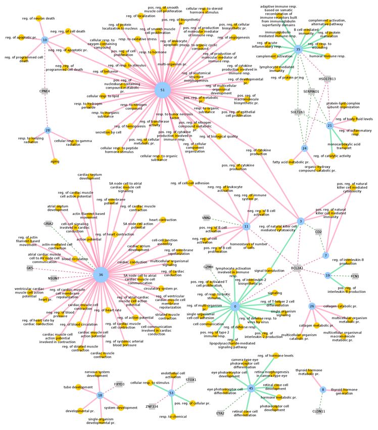
differences between healthy and diseased arteries (Figure 5). For instance, clusters
3 and 7 present a strong enrichment in AAW for the regulation of natural killer
(NK) cells that augment atherosclerosis by cytotoxic-dependent mechanisms [49].
In IMA, these clusters are predicted to be regulated by genetic variation in CD2, a
cell adhesian molecule found on the surface of T and NK cells, whereas in AAW
their predicted regulator is BCL2A1, an important cell death regulator and pro-
inflammatory gene that is upregulated in coronary plaques compared to healthy con-
trols [50]. This suggests that misregulation of cytotoxic response processes plays a
role in the disease, further supported by the overrepresentation in cluster 10 of genes
associated with cell death that are a important trigger of plaque rupture [51]. Fur-
thermore, variations in BCL2A1 are predicted to regulate other clusters exclusively
in AAW too, with disease-relevant AAW enrichments. Cluster 11 is associated with
the regulation of B lymphocytes, which may attenuate the neointimal formation of
atherosclerosis [52], while cluster 26 is enriched for collagen production regula-
tion. Uncontrolled collagen accumulation leads to arterial stenosis, while excessive
collagen breakdown combined with inadequate synthesis weakens plaques thereby
making them prone to rupture [53]. Last, as expected, terms related with the heart,
cardiac muscle and blood circulation are strongly enriched in AAW, in particular
in cluster 36. In AAW, this cluster is regulated by GK5, which plays an important
role in fatty acid metabolism and whose upregulation has previously been associ-
ated to the pathogenesis of atherosclerosis and cardiovascular disease in patients
with auto-immune conditions [54]. On the opposite side, cluster 36 in IMA is regu-
lated by GRIA2, a player in the ion transport pathway, which has been shown to be
down-regulated in advanced atherosclerotic lesions [55].
In summary, this application has shown that differential module network infer-
ence allows to identify sets of one-to-one mapping modules representing broad bi-
ological processes conserved between conditions, with biologically relevant differ-
ences in fine-grained gene-to-module assignments and upstream regulatory factors.Learning differential module networks across multiple experimental conditions 15 Fig. 5 Tissue-specific GO enrichment for terms related to the immune system process (GO0002376) and regulator assignment in the STAGE AAW-IMA differential module net- work. Reassignment of nodes was computed with a threshold of 0.015. Blue nodes are modules, yellow nodes GO terms, grey nodes regulatory genes. Red and green edges indicate tissue-specific enrichment (q < 0.01) in the corresponding AAW and IMA module, respectively. Dashed red and green edges indicate regulator assignments in AAW and IMA, respectively. Only top 1% regulators are depicted. neg., negative; pos., positive; pr., process; reg., regulation; resp., response.
16                                                       Pau Erola, Eric Bonnet and Tom Michoel

Acknowledgements PE and TM are supported by Roslin Institute Strategic Programme funding
from the BBSRC [BB/P013732/1].

References

 1. M E J Newman. Modularity and community structure in networks. PNAS, 103:8577–8582,
    2006.
 2. L H Hartwell, J J Hopfield, S Leibler, and A W Murray. From molecular to modular cell
    biology. Nature, 402:C47–C52, 1999.
 3. Y Qi and H Ge. Modularity and dynamics of cellular networks. PLoS Comput Biol, 2:e174,
    2006.
 4. Michael B Eisen, Paul T Spellman, Patrick O Brown, and David Botstein. Cluster analysis
    and display of genome-wide expression patterns. PNAS, 95(25):14863–14868, 1998.
 5. P T Spellman, G Sherlock, M Q Zhang, V R Iyer, K Anders, M B Eisen, P O Brown, D Bot-
    stein, and B Futcher. Comprehensive identification of cell cycle-regulated genes of the yeast
    Saccharomyces cerevisiae by microarray hybridization. Mol Biol Cell, 9:3273–3297, 1998.
 6. E Segal, M Shapira, A Regev, D Pe’er, D Botstein, D Koller, and N Friedman. Module net-
    works: identifying regulatory modules and their condition-specific regulators from gene ex-
    pression data. Nat Genet, 34:166–167, 2003.
 7. N Friedman. Inferring cellular networks using probabilistic graphical models. Science,
    308:799–805, 2004.
 8. D Koller and N Friedman. Probabilistic Graphical Models: Principles and Techniques. The
    MIT Press, 2009.
 9. S.I. Lee, D. Pe’er, A.M. Dudley, G.M. Church, and D. Koller. Identifying regulatory mecha-
    nisms using individual variation reveals key role for chromatin modification. Proc. Natl. Acad.
    Sci. U.S.A., 103:14062–14067, Sep 2006.
10. Wei Zhang, Jun Zhu, Eric E Schadt, and Jun S Liu. A Bayesian partition method for detecting
    pleiotropic and epistatic eQTL modules. PLoS Computational Biology, 6(1):e1000642, 2010.
11. Su-In Lee, Aimée M Dudley, David Drubin, Pamela A Silver, Nevan J Krogan, Dana Pe’er,
    and Daphne Koller. Learning a prior on regulatory potential from eqtl data. PLoS Genetics,
    5(1):e1000358, 2009.
12. E. Bonnet, M. Tatari, A. Joshi, T. Michoel, K. Marchal, G. Berx, and Y. Van de Peer. Network
    inference from a cancer gene expression data set identifies microRNA regulated modules.
    PLoS One, 5:e10162, 2010.
13. E. Bonnet, T. Michoel, and Y. Van de Peer. Prediction of a gene regulatory network linked to
    prostate cancer from gene expression, microRNA and clinical data. Bioinformatics, 26:i683–
    i644, 2010.
14. U D Akavia, O Litvin, J Kim, F Sanchez-Garcia, D Kotliar, H C Causton, P Pochanard,
    E Mozes, L A Garraway, and Pe’er D. An integrated approach to uncover drivers of can-
    cer. Cell, 143:1005–1017, 2010.
15. Eric Bonnet, Laurence Calzone, and Tom Michoel. Integrative multi-omics module network
    inference with Lemon-Tree. PLoS Computational Biology, 11(2):e1003983, 2015.
16. Noa Novershtern, Aviv Regev, and Nir Friedman. Physical module networks: an integrative
    approach for reconstructing transcription regulation. Bioinformatics, 27(13):i177–i185, 2011.
17. T Michoel, R De Smet, A Joshi, Y Van de Peer, and K Marchal. Comparative analysis of
    module-based versus direct methods for reverse-engineering transcriptional regulatory net-
    works. BMC Syst Biol, 3:49, 2009.
18. Sushmita Roy, Stephen Lagree, Zhonggang Hou, James A Thomson, Ron Stewart, and Au-
    drey P Gasch. Integrated module and gene-specific regulatory inference implicates upstream
    signaling networks. PLoS Computational Biology, 9(10), 2013.
Learning differential module networks across multiple experimental conditions 17
19. E Segal, C B Sirlin, C Ooi, A S Adler, J Gollub, X Chen, B K Chan, G R Matcuk, C T Barry,
H Y Chang, and M D Kuo. Decoding global gene expression programs in liver cancer by
noninvasive imaging. Nat Biotech, 25:675–680, 2007.
20. H Zhu, H Yang, and M R Owen. Combined microarray analysis uncovers self-renewal related
signaling in mouse embryonic stem cells. Syst Synth Biol, 1:171–181, 2007.
21. J. Li, Z.J. Liu, Y.C. Pan, Q. Liu, X. Fu, N.G. Cooper, Y.X. Li, M.S. Qiu, and T.L. Shi. Regula-
tory module network of basic/helix-loop-helix transcription factors in mouse brain. Genome
Biol, 8:R244, Nov 2007.
22. N Novershtern, Z Itzhaki, O Manor, N Friedman, and N Kaminski. A functional and regulatory
map of asthma. Am J Respir Cell Mol Biol, 38:324–336, 2008.
23. I Amit, M Garber, N Chevrier, A P Leite, Y Donner, T Eisenhaure, M Guttman, J K Grenier,
W Li, O Zuk, L A Schubert, B Birditt, T Shay, A Goren, X Zhang, Z Smith, R Deering,
R C McDonald, M Cabili, B E Bernstein, J L Rinn, A Meissner, D E Root, N Hacohen,
and A Regev. Unbiased reconstruction of a mammalian transcriptional network mediating
pathogen responses. Science, 326:257, 2009.
24. V. Vermeirssen, A. Joshi, T. Michoel, E. Bonnet, T. Casneuf, and Y. Van de Peer. Transcription
regulatory networks in Caenorhabditis elegans inferred through reverse-engineering of gene
expression profiles constitute biological hypotheses for metazoan development. Mol. BioSyst.,
5:1817–1830, 2009.
25. Noa Novershtern, Aravind Subramanian, Lee N Lawton, Raymond H Mak, W Nicholas
Haining, Marie E McConkey, Naomi Habib, Nir Yosef, Cindy Y Chang, Tal Shay, et al.
Densely interconnected transcriptional circuits control cell states in human hematopoiesis.
Cell, 144(2):296–309, 2011.
26. Mingzhu Zhu, Xin Deng, Trupti Joshi, Dong Xu, Gary Stacey, and Jianlin Cheng. Recon-
structing differentially co-expressed gene modules and regulatory networks of soybean cells.
BMC Genomics, 13(1):437, 2012.
27. Stilianos Arhondakis, Craita E Bita, Andreas Perrakis, Maria E Manioudaki, Afroditi Krokida,
Dimitrios Kaloudas, and Panagiotis Kalaitzis. In silico transcriptional regulatory networks
involved in tomato fruit ripening. Frontiers in plant science, 7, 2016.
28. Elham Behdani and Mohammad Reza Bakhtiarizadeh. Construction of an integrated gene
regulatory network link to stress-related immune system in cattle. Genetica, 145(4-5):441–
454, 2017.
29. Fabio Albuquerque Marchi, David Correa Martins, Mateus Camargo Barros-Filho, Hellen
Kuasne, Ariane Fidelis Busso Lopes, Helena Brentani, Jose Carlos Souza Trindade Filho,
Gustavo Cardoso Guimarães, Eliney F Faria, Cristovam Scapulatempo-Neto, et al. Multidi-
mensional integrative analysis uncovers driver candidates and biomarkers in penile carcinoma.
Scientific Reports, 7, 2017.
30. Alberto de la Fuente. From ‘differential expression’ to ‘differential networking’–identification
of dysfunctional regulatory networks in diseases. Trends in Genetics, 26(7):326–333, 2010.
31. Trey Ideker and Nevan J Krogan. Differential network biology. Molecular Systems Biology,
8(1):565, 2012.
32. Gennaro Gambardella, Maria Nicoletta Moretti, Rossella De Cegli, Luca Cardone, Adri-
ano Peron, and Diego Di Bernardo. Differential network analysis for the identification of
condition-specific pathway activity and regulation. Bioinformatics, 29(14):1776–1785, 2013.
33. Min Jin Ha, Veerabhadran Baladandayuthapani, and Kim-Anh Do. DINGO: differential net-
work analysis in genomics. Bioinformatics, 31(21):3413–3420, 2015.
34. Andrew T McKenzie, Igor Katsyv, Won-Min Song, Minghui Wang, and Bin Zhang. DGCA:
A comprehensive r package for differential gene correlation analysis. BMC systems biology,
10(1):106, 2016.
35. André Voigt, Katja Nowick, and Eivind Almaas. A composite network of conserved and
tissue specific gene interactions reveals possible genetic interactions in glioma. PLOS Com-
putational Biology, 13(9):e1005739, 2017.
36. Sushmita Roy, Ilan Wapinski, Jenna Pfiffner, Courtney French, Amanda Socha, Jay
Konieczka, Naomi Habib, Manolis Kellis, Dawn Thompson, and Aviv Regev. Arboretum:18 Pau Erola, Eric Bonnet and Tom Michoel
reconstruction and analysis of the evolutionary history of condition-specific transcriptional
modules. Genome Research, 23(6):1039–1050, 2013.
37. A Joshi, R De Smet, K Marchal, Y Van de Peer, and T Michoel. Module networks revisited:
computational assessment and prioritization of model predictions. Bioinformatics, 25(4):490–
496, 2009.
38. E Segal, D Pe’er, A Regev, D Koller, and N Friedman. Learning module networks. Journal of
Machine Learning Research, 6:557–588, 2005.
39. T Michoel, S Maere, E Bonnet, A Joshi, Y Saeys, T Van den Bulcke, K Van Leemput, P van
Remortel, M Kuiper, K Marchal, and Y Van de Peer. Validating module networks learning
algorithms using simulated data. BMC Bioinformatics, 8:S5, 2007.
40. ZS Qin. Clustering microarray gene expression data using weighted chinese restaurant pro-
cess. Bioinformatics, 22:1988–1997, 2006.
41. A Joshi, Y Van de Peer, and T Michoel. Analysis of a Gibbs sampler for model based cluster-
ing of gene expression data. Bioinformatics, 24(2):176–183, 2008.
42. Youtao Lu, Xiaoyuan Zhou, and Christine Nardini. Dissection of the module network imple-
mentation “LemonTree”: enhancements towards applications in metagenomics and translation
in autoimmune maladies. Molecular BioSystems, 13(10):2083–2091, 2017.
43. T. Michoel and B. Nachtergaele. Alignment and integration of complex networks by
hypergraph-based spectral clustering. Physical Review E, 86:056111, 2012.
44. S Maere, K Heymans, and M Kuiper. BiNGO: a Cytoscape plugin to assess overrepresentation
of gene ontology categories in biological networks. Bioinformatics, 21:3448–3449, 2005.
45. S. Hägg, J. Skogsberg, J. Lundström, P. Noori, R. Nilsson, H. Zhong, S. Maleki, M. M.
Shang, B. Brinne, M. Bradshaw, V. B. Bajic, A. Samnegard, A. Silveira, L. M. Kaplan, B. Gi-
gante, K. Leander, U. de Faire, S. Rosfors, U. Lockowandt, J. Liska, P. Konrad, R. Takolan-
der, A. Franco-Cereceda, E. E. Schadt, T. Ivert, A. Hamsten, J. Tegner, and J. Björkegren.
Multi-organ expression profiling uncovers a gene module in coronary artery disease involv-
ing transendothelial migration of leukocytes and LIM domain binding 2: the Stockholm
Atherosclerosis Gene Expression (STAGE) study. PLoS Genetics, 5(12):e1000754, Dec 2009.
46. H. Foroughi Asl, H Talukdar., A. Kindt, R. Jain, R. Ermel, A. Ruusalepp, K.-D. Nguyen,
R. Dobrin, D. Reilly, CARDIoGRAM Consortium, H. Schunkert, N. Samani, I. Braenne,
J. Erdmann, O. Melander, J. Qi, T. Ivert, J. Skogsberg, E. E. Schadt, T. Michoel, and
J. Björkegren. Expression quantitative trait loci acting across multiple tissues are enriched in
inherited risk of coronary artery disease. Circulation: Cardiovascular Genetics, 8:305–315,
2015.
47. H. Talukdar, H Foroughi Asl, R. Jain, R. Ermel, A. Ruusalepp, O. Franzén, B. Kidd, B. Read-
head, C. Giannarelli, T. Ivert, J. Dudley, M. Civelek, A. Lusis, E. Schadt, J. Skogsberg, T. Mi-
choel, and J.L.M Björkegren. Cross-tissue regulatory gene networks in coronary artery dis-
ease. Cell Systems, 2:196–208, 2016.
48. E E Schadt. Molecular networks as sensors and drivers of common human diseases. Nature,
461:218–223, 2009.
49. Ahrathy Selathurai, Virginie Deswaerte, Peter Kanellakis, Peter Tipping, Ban-Hock Toh,
Alex Bobik, and Tin Kyaw. Natural killer (NK) cells augment atherosclerosis by cytotoxic-
dependent mechanisms. Cardiovascular research, 102(1):128–137, 2014.
50. Krzysztof Sikorski, Joanna Wesoly, and Hans AR Bluyssen. Data mining of atherosclerotic
plaque transcriptomes predicts STAT1-dependent inflammatory signal integration in vascular
disease. International journal of molecular sciences, 15(8):14313–14331, 2014.
51. Wim Martinet, Dorien M Schrijvers, and Guido RY De Meyer. Pharmacological modulation
of cell death in atherosclerosis: a promising approach towards plaque stabilization? British
Journal of Pharmacology, 164(1):1–13, 2011.
52. Breanne N Gjurich, Parésa L Taghavie-Moghadam, Klaus Ley, and Elena V Galkina. L-
selectin deficiency decreases aortic B1a and Breg subsets and promotes atherosclerosis.
Thrombosis and Haemostasis, 112(4):803, 2014.
53. Mark D Rekhter. Collagen synthesis in atherosclerosis: too much and not enough. Cardiovas-
cular Research, 41(2):376–384, 1999.Learning differential module networks across multiple experimental conditions 19
54. Carlos Perez-Sanchez, Nuria Barbarroja, Sebastiano Messineo, Patricia Ruiz-Limon, Anto-
nio Rodriguez-Ariza, Yolanda Jimenez-Gomez, Munther A Khamashta, Eduardo Collantes-
Estevez, Ma Jose Cuadrado, Ma Angeles Aguirre, et al. Gene profiling reveals specific molec-
ular pathways in the pathogenesis of atherosclerosis and cardiovascular disease in antiphos-
pholipid syndrome, systemic lupus erythematosus and antiphospholipid syndrome with lupus.
Annals of the rheumatic diseases, 74(7):1441–1449, 2015.
55. Shijun Fu, Haiguang Zhao, Jiantao Shi, Arhat Abzhanov, Keith Crawford, Lucila Ohno-
Machado, Jianqin Zhou, Yanzhi Du, Winston Patrick Kuo, Ji Zhang, et al. Peripheral arte-
rial occlusive disease: global gene expression analyses suggest a major role for immune and
inflammatory responses. Bmc Genomics, 9(1):369, 2008.You can also read