Learning to Generate Maps from Trajectories
←
→
Page content transcription
If your browser does not render page correctly, please read the page content below
Learning to Generate Maps from Trajectories∗
                       Sijie Ruan1,2,3 , Cheng Long4 , Jie Bao2,3 , Chunyang Li1 , Zisheng Yu1
                           Ruiyuan Li1,2,3 , Yuxuan Liang5 , Tianfu He6,2,3 , Yu Zheng1,2,3
                          1
                            School of Computer Science and Technology, Xidian University, Xi’an, China
        2
            JD Intelligent Cities Research, Beijing, China 3 JD Intelligent Cities Business Unit, JD Digits, Beijing, China
                   4
                     School of Computer Science and Engineering, Nanyang Technological University, Singapore
                                 5
                                   School of Computing, National University of Singapore, Singapore
                   6
                     School of Computer Science and Technology, Harbin Institute of Technology, Harbin, China
                      {sjruan, yuzisheng}@stu.xidian.edu.cn, c.long@ntu.edu.sg, {baojie, ruiyuan.li}@jd.com
                                  {lichunyang 1, yuxliang, Tianfu.D.He, msyuzheng}@outlook.com

                              Abstract
  Accurate and updated road network data is vital in many
  urban applications, such as car-sharing, and logistics. The
  traditional approach to identifying the road network, i.e.,
  field survey, requires a significant amount of time and ef-
  fort. With the wide usage of GPS embedded devices, a
  huge amount of trajectory data has been generated by dif-
  ferent types of mobile objects, which provides a new op-                  (a) GT.             (b) Point.             (c) Line.
  portunity to extract the underlying road network. However,
  the existing trajectory-based map recovery approaches re-                           Figure 1: Motivation Examples.
  quire many empirical parameters and do not utilize the prior
  knowledge in existing maps, which over-simplifies or over-
  complicates the reconstructed road network. To this end, we
  propose a deep learning-based map generation framework,             two consecutive GPS points of the dataset. As could be no-
  i.e., DeepMG, which learns the structure of the existing road       ticed, using the point cloud for map generation would be
  network to overcome the noisy GPS positions. More specifi-          incapable of distinguishing parallel roads that are spatially
  cally, DeepMG extracts features from trajectories in both spa-      close and using the line segments for map generation would
  tial view and transition view and uses a convolutional deep
                                                                      result in many redundant edges. And such a case would be
  neural network T2RNet to infer road centerlines. After that, a
  trajectory-based post-processing algorithm is proposed to re-       even worse if the sampling rate decreases.
  fine the topological connectivity of the recovered map. Exten-         Despite the challenges of map generation, many meth-
  sive experiments on two real-world trajectory datasets con-         ods have been developed for this problem, which can
  firm that DeepMG significantly outperforms the state-of-the-        be categorized into three classes: 1) Clustering-based ap-
  art methods.                                                        proach (Edelkamp and Schrödl 2003; Chen et al. 2016;
                                                                      Stanojevic et al. 2018), which first generates a set of road
                        Introduction                                  ends using some clustering algorithm based on geospa-
                                                                      tial distances and direction similarities and then links the
With the increased population mobility and the rising of car-         road ends as road segments by using trajectories; 2) Trace-
sharing service, accurate and updated road network data be-           merging based approach (Cao and Krumm 2009), which
comes vital. Conventional approaches for collecting road              scans trajectories sequentially and for each one, either
network data such as field surveys are costly and labor-              merges it to some existing road segments or generates some
intensive. With the wide usage of GPS embedded devices,               new road segments if no suitable merging operations are
a huge amount of trajectory data has been generated by dif-           possible; 3) Kernel density estimation (KDE) based ap-
ferent types of mobile objects (Zheng et al. 2014), which             proach (Biagioni and Eriksson 2012b; Wang, Wang, and
provides a new opportunity to extract the underlying road             Li 2015), which performs KDE on the point cloud and ex-
network. Yet, generating a map from trajectories is a non-            tracts a map afterward. While these existing methods pro-
trivial task, which is mainly because trajectories usually in-        vide some insights for map generation, they still suffer from
volve GPS noises and are collected with different sampling            various types of issues. Consider the clustering-based and
rates. To illustrate this, we present in Fig 1 a) the map near        trace-merging based approaches. Since they generate road
a roundabout area in Beijing, b) the GPS point cloud based            segments somehow based on the line segments between con-
on a taxi trajectory dataset and c) the line segments between         secutive points, in cases that trajectories are sampled with
   ∗
     Yu Zheng and Jie Bao are corresponding authors.                  low rates, they would generate many shortcuts that do not
Copyright c 2020, Association for the Advancement of Artificial       exist in a real map. Besides, these approaches are ineffec-
Intelligence (www.aaai.org). All rights reserved.                     tive in distinguishing parallel road segments towards the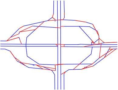
same direction, which is mainly because they provide not                             Geometry Translation                             Topology Construction

                                                                    Inference
many mechanisms for handling GPS noises in trajectory                                           Feature            Trained               …            Map
data. Consider the KDE based approach. While it has the                                        Extraction           Model                          Refinement
                                                                                                                         Centerline
capability of handling low-sampling trajectories (since it is                                                                          Graph
                                                                                 Feature                     predictions

                                                                    Training
based on point clouds), it would often merge several parallel                   Extraction                                            Extraction
                                                                                             T2RNet         loss
roads that are close to one another into a single one.                                                                                  Link
   In this paper, we propose a Deep learning-based Map                          Trajectory                         Map                Generation

Generation framework (DeepMG) to generate routable maps
from trajectories, which can handle trajectories with differ-                           Figure 2: The Framework of DeepMG.
ent sampling rates and distinguish parallel road segments
leveraging the knowledge of existing maps. The key con-
tributions of this paper can be summarized as follows:                                       Geometry Translation
• We propose the first deep learning-based approach for            Feature Extraction
   generating routable maps from trajectories, which enjoys
                                                                   Similar to some tasks for aerial image segmentation (Demir
   various superiorities over existing approaches.
                                                                   et al. 2018), we split the region of interest into tiles and re-
• We design the map generation framework DeepMG, con-              gard each tile as a data sample. For each tile, we partition it
   sisting of two modules: 1) geometry translation, which          into a grid with I × J cells and for each grid cell, we extract
   extracts features in trajectories from two views and            some features from the trajectories in two views, namely the
   then feeds the features into a Trajectory-Road transla-         spatial view and the transition view.
   tion model called T2RNet for predicting road centerlines        Spatial View. In the spatial view, the features of a grid cell
   (which correspond to line segments on a map). 2) topol-         are based on the trajectory data within the cell. Specifically,
   ogy construction, which extracts a graph structure from         we consider four types of features: 1) Point, which is the
   the predicted centerlines, links among those dead ends of       GPS point density of a grid cell (we use one of the three
   edges for better connectivity and then refines the graph        equal quantiles of point densities). The Point feature is the
   structure (map) by using the trajectory data.                   most straightforward indicator of the underlying roads. 2)
• We conduct extensive experiments as well as case stud-           Line: the number of line segments in each grid cell, which
   ies on two real-world taxi trajectory datasets. Experiments     are generated from two consecutive points in trajectories (we
   show DeepMG significantly outperforms the state-of-the-         use normalized values in the range [0,1]). The Line feature
   art map reconstruction algorithms.                              could help with recovering the roads when points are sparse.
                                                                   3) Speed, which is the average moving speed in a grid cell.
                         Overview                                  The speeds are inferred based on consecutive points, which
                                                                   could help with recovering a road segment completely since,
Preliminary
                                                                   on the same road, the speed usually does not change that
Definition 1 (Trajectory). A trajectory is a sequence of           much. 4) Direction, which captures the moving directions
spatio-temporal points, denoted as tr =< p1 , p2 , ..., pn >,      within a grid cell. We consider 8 regular directions (e.g.,
where each point p = (x, y, t) consists of a location (x, y)       north, northeast, etc.), count the occurrences of each direc-
(e.g., longitude and latitude) at time t. Points in a trajectory   tion for a movement between two consecutive points, and
are organized chronologically, namely, ∀i < j : pi .t < pj .t.     then normalize the counts into a histogram. The direction
Definition 2 (Map). A map is a directed graph, denoted as          feature could be helpful for distinguishing two parallel roads
G =< V, E >, where each vertex v ∈ V is associated with a          in opposite directions. In each grid cell, we can obtain an 11-
location (x, y), and each edge e ∈ E is a vertex tuple (u, v),     dimensional vector with the above features, and the spatial
denoting the connectivity from u to v.                             view of the grid could be denoted as Xs ∈ R11×I×J .
Definition 3 (Map Matching). Map matching is a process             Transition View. In the transition view, the features of a grid
of inferring the underlying sequence of edges e1 → e2 →            cell are based on the trajectory data that spans over this cell
· · · → en for a given trajectory tr based on a certain map.       and some other cells. The features in this view are essential
                                                                   especially for the trajectories with low sampling rates since
Problem Statement. Given a set of trajectories T             =     in these cases, the two consecutive points would be often lo-
{tr1 , tr2 , · · · , trn }, infer its underlying map G.            cated in different cells, which further implies that many fea-
                                                                   tures in the spatial view such as Line, Speed and Direction
Framework                                                          would have limited usage. Specifically, for a grid cell c, we
The overview of our map generation framework DeepMG is             consider those neighboring cells c0 such that there exist two
presented in Fig 2, which is comprised of two steps: 1) Ge-        consecutive points which are from c0 to c. We capture these
ometry Translation, which extracts features from trajectory        cells c0 with a binary matrix such that the entry correspond-
data and then feeds the features to T2RNet for predicting the      ing to c0 is set to 1 if there exist two consecutive points which
road centerlines; 2) Topology Construction, which extracts a       are from c0 to c, and 0 otherwise. Besides, we consider those
graph structure from the predicted road centerlines, gener-        cells c00 such that there exist two consecutive points which
ates some extra links for better connectivity and then refines     are from c to c00 and capture the cells with another binary
the graph structure using the trajectory data again.               matrix similarly as we do for cells c0 . These two matrices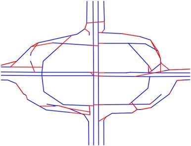
then correspond to the features in the transition view. Note
Embedding
Transition
that these two matrices would usually be very sparse, which
Dense
Dense
ReLU
ReLU
ReLU
Conv
ReLU
Conv
BN
BN
could degrade the effectiveness of using these features. To
mitigate this issue, we control the neighborhood area by a ConvBlock
Transition View
distance parameter, and use a lower resolution for forming
cells c0 and c00 . We denote the neighborhood size of c as
ConvBlock
ConvBlock
ConvBlock
MaxPool
MaxPool
Encoder
EM
Shared
T × T , and the features in the transition view could be de- E1
... ...
noted as Xt ∈ Z22×T ×T ×I×J , where Z2 means the set of
binary values {0, 1}. Spatial View
Road Region
ConvBlock
ConvBlock
ConvTrans
ConvTrans
T2RNet
Sigmoid
Decoder
...
ReLU
ReLU
Conv
Recall that the task of the geometry translation module is to
predict the road centerlines of a map from trajectory data. Region RD1 RDM
An intuitive idea is to model this task as a pixel-wise image
Road Centerline
ConvTrans
ConvTrans
ConvBlock
ConvBlock
classification one and then utilize existing models for the
Sigmoid
Decoder
...
ReLU
ReLU
Conv
task. However, due to the fact that a typical road centerline
would be single-pixel wide, which is too shallow for conven-
Centerline
tional image classification models to be effective. Motivated
by this, we introduce an auxiliary task to support the task Figure 3: T2RNet Architecture.
of road centerline prediction. Specifically, the auxiliary task
is to predict the spatial regions that involve roads, which we
call road regions. We call this auxiliary task road region pre- EM +1 passes through M upsampling blocks. Each upsam-
diction. Note that the task of road region prediction should pling block first uses a transposed convolution layer (Con-
be easier than that of road centerline prediction since for the vTrans) followed by a ReLU for the upsampling purpose. Its
former task, the targets are wider and existing image clas- m−1 I
F × m−1 J
× m−1
sification models could be effectively utilized. Specifically, output RDm ∈ R2 2 2 is concatenated with
we propose a multi-task learning architecture called T2RNet Em , and then fed into a ConvBlock for information fusion.
whose overview is presented in Fig 3. T2RNet involves four Finally, a convolution layer (3×3, 1) and a Sigmoid activa-
components, namely (1) transition embedding, (2) shared tion are applied to generate the final road region prediction.
encoder, (3) road region decoder, and (4) road centerline (4) Road Centerline Decoder. This is to predict the road
decoder, with details explained next. centerline leveraging both the encoded information and the
(1) Transition Embedding. This component is motivated information from road region decoder (i.e., the road center-
by that the features in the transition view, captured by Xt , line prediction task). The idea is similar to that of the road
could be very sparse since objects usually move from and region decoder except that during the information fusion in
to a limited number of cells nearby. Inspired by the idea of each layer, we concatenate not only the information from
word embedding (Mikolov et al. 2013), we first use dense the encoder, i.e., Em , but also that from the road region de-
layers to transform Xt into a dense representation Ht ∈ coder, i.e., RDm , so that the learned road region informa-
Rk×I×J and the structure is depicted in the top left of Fig 3, tion would help with the road centerline prediction task.
where k is the size of the embedded dimension. Optimization. For each edge in the map, we use a one-pixel
(2) Shared Encoder. The shared encoder, which is shared wide line segment linking its two ends as a road centerline.
by two decoders, is used to encode the features at differ- The tile of road centerlines is denoted as Yc ∈ ZI×J 2 . We
ent levels. Specifically, the concatenation of Xs and Ht also mask nearby grids around the road centerlines to gener-
is passed to M downsampling blocks. Each downsampling ate the labels of road region Yr ∈ ZI×J 2 . Since the positive
block contains a ConvBlock and a Max Pooling layer. The and the negative labels are extremely imbalanced for Yc and
structure of the ConvBlock, as shown on the top right of Yr , we employ the Dice loss (Milletari, Navab, and Ahmadi
Fig 3, contains two 3×3 convolutional layers, and there 2016), which is designed for tackling small foreground is-
are F filters in the first ConvBlock, which are doubled af- sues, as our loss function. Specifically, the Dice loss of the
ter each downsampling. In the ConvBlock, each convolu- prediction Ŷ given the ground truth Y is:
tional layer is followed by a Batch Normalization (Ioffe
and Szegedy 2015), with a ReLU to introduce non-linearity. PI PJ
We denote the feature map after a ConvBlock as Em ∈ 2 i j Ŷij Yij +
m−1 I J
LDice (Ŷ, Y) = 1 − PI PJ PI PJ (1)
F × m−1 × m−1
R2 2 2 , where m = 1, · · · , M , and Em is i j Ŷij + i j Yij +
downsampled by half after the Max Pooling layer. Finally,
where the term is used to ensure the loss function stability
another ConvBlock, which serves as the bottleneck layer, is
by avoiding the numerical issue of being divided by 0.
used to produce the final feature map EM +1 .
We minimize the hybrid Dice loss of road centerline pre-
(3) Road Region Decoder. This is to predict the road re- diction and road region prediction by gradient descent.
gions given the encoded information from the shared en-
coder (i.e., the road region prediction task). Specifically, L(θ) = (1 − λ)LDice (Ŷc , Yc ) + λLDice (Ŷr , Yr ) (2)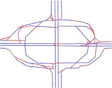
where θ are all trainable parameters and λ is the hyperpa- Algorithm 1 Link Generation.
rameter that balances two types of loss. Input: Initial undirected map G; link radius Rlink .
Output: Linked undirected map G.
Topology Construction 1: Vnew ← ∅, Enew ← ∅;
2: for v ∈ G.V do
While the geometry translation module can predict the 3: if deg(v) = 1 then
road centerlines, the topological connectivity can not be 4: u ← get adjacent vertex(v);
guaranteed. Many techniques for connecting broken edges 5: C ← get neighboring edges(v, Rlink );
have been proposed in the literature of aerial imagery road 6: for e ∈ C do
detection (Mnih 2013; Máttyus, Luo, and Urtasun 2017; 7: t ← cal intersection point(u, v, e);
Sun et al. 2018). Nevertheless, these techniques are inca- 8: if t 6= null then
pable of inferring the directions of roads or guaranteeing the 9: Vnew ← Vnew ∪{t}, Enew ← Enew ∪{(v, t)};
connection between two edges that are truly linked. Differ- 10: else
ing from these studies, we use trajectories as evidence for 11: n ← the nearest vertex of e to v;
12: if deg(n) = 1 and angle(− → −
uv, → ≤ 90◦ then
vn)
constructing the topology of a map, which links broken road 13: Enew ← Enew ∪ {(v, n)};
segments and infers the directions simultaneously. Specif-
14: for v ∈ Vnew do
ically, our solution involves three steps: namely 1) graph
15: split the edge, on which v is located; add v to G;
extraction, which extracts an initial map from the predicted
16: for e ∈ Enew do
road centerlines; 2) link generation, which generates all pos-
17: add e to G;
sible transition links among dead ends of edges; 3) map re-
18: return G;
finement, which refines the map further based on trajectories.
Graph Extraction Path 1:
e2
In this step, we concatenate all predicted road centerlines e1 P1 e1
b Path 2:
based on their underlying tiles. Then we adopt the com-
Od a
bustion technique (Shi, Shen, and Liu 2009) to construct an
initial undirected map from the predicted centerlines, where e3 l3 l1
each road centerline would have a corresponding edge. P2
e2
e3 l2
(a) Link Generation. (b) Undesired Shortcuts.
Link Generation
In this step, we use a heuristic algorithm to generate all pos- Figure 4: Topology Construction Illustration.
sible links among dead ends of edges nearby. The pseudo
code is given in Algorithm 1. Since a road edge is straight,
the generated links should also be smooth when linking bro- are not traversed through often. Specifically, we perform tra-
ken edges. Therefore, we generate a link from each dead end jectory map matching (Yuan et al. 2010b) to map the tra-
v of an edge within a radius Rlink in the following two cases. jectories to the current map. We note that directly apply-
• The extension of the edge starting from v intersects an- ing existing methods is not sufficient for the map refinement
other edge. In this case, we create a new vertex at the in- purpose here since they usually assume that moving objects
tersection t, and generate a link between v and t (Line 9). follow the shortest paths between consecutive points, which
would cause problems as illustrated in Fig 4b. In the figures,
• The intersection point does not exist, but the nearest ver- the solid lines are predicted edges, and the dash lines are
tex n of the edge to v is a dead end, and there could be a generated links. During map matching, if e1 is a candidate
smooth transition from v to n (e.g., the turning direction road to match for P1 and e3 is a candidate road for P2 , then
is not greater than 90◦ ). In this case, we generate a link the algorithm uses Path 1 to capture the transition probabil-
between v and n (Line 13). ity from e1 to e2 since this corresponds to the shortest path.
In detail, we first create two sets Vnew and Enew to record However, Path 2 is much more likely an actual path, since
vertices and links that will be added to the map (Line 1). the edges are more reliable than links. Therefore, we use the
After all dead ends are examined, each vertex in Vnew is edge length multiplied by a penalty factor α (α > 1) as the
added and used to split an existing edge on which the vertex edge weight for created links so that the shortest path calcu-
is located on and each link in Enew is added (Line 14-17). lation will prefer edges over generated links.
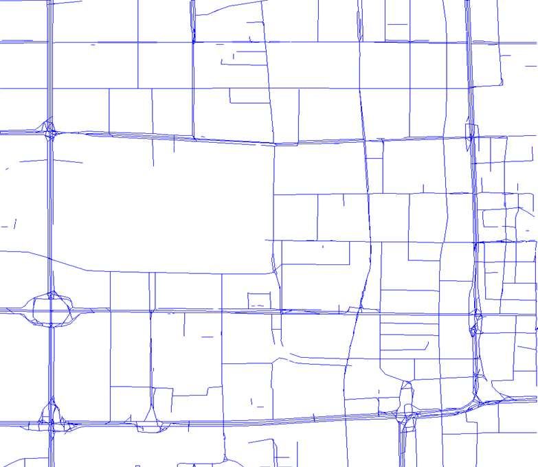
As shown in Fig 4a, we generate a link between o and a After we have matched all trajectories on the map, the
on e1 and another link between o and b of e2 (the turning inferred paths are used as evidence of the transition. We re-
from o to e2 is smooth). Note that we do not generate a link move those edges or generated links who witness less than
from o to e3 since its transition to e3 is not smooth. S times of transitions, and obtain the refined directed map.
Map Refinement Experiments
In this step, we refine the map further based on trajectories. In this section, we report the overall performance of
The main idea is to remove edges and generated links that DeepMG, following by the performance of its two modules.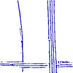
Experimental Settings                                                inferred by clustering and edges are created by trajecto-
                                                                     ries, a graph sparsification step is used to simplify the
Datasets. We use two real-world taxi trajectory datasets, i.e.,
                                                                     graph. To the authors’ knowledge, this is the state-of-the-
TaxiBJ and TaxiJN, with different sampling rates for evalu-
                                                                     art method for map reconstruction.
ations. TaxiBJ is obtained from T-Drive (Yuan et al. 2010a)
and TaxiJN is a private one donated by the government of           • Cao (Cao and Krumm 2009), which is a trace-merging
Jinan. Several preprocessing algorithms, e.g., noise filtering,      based algorithm. The main idea is to reduce GPS noises
stay point removal (Zheng 2015), are applied. The detailed           based on particle simulation. It uses a strong but short-
statistics of the datasets are given in Tab 1, where the statis-     range force to pull together nearby traces, and a weaker
tics of the test region are given in the parentheses. Each sam-      but long-range force to keep traces from straying too far.
ple is a 256×256 grid, and each cell is 2m×2m, which is the        • Biagioni (Biagioni and Eriksson 2012b), which is a KDE
coarsest resolution so that two parallel centerlines are distin-     based approach. It converts the trajectory points into a
guishable. The number of samples for training, validation,           road network skeleton image in different confidence lev-
and test are 744, 180, 100 for TaxiBJ, and 1251, 313, 100            els based on KDE, and then a density-aware map match-
for TaxiJN. The baselines are only compared in the test re-          ing algorithm is used to remove low support edges.
gion. We use OpenStreetMap as the ground truth, and road
region labels are generated by masking 2 cells surrounding            We also compare the performance of DeepMG without
the centerlines. We remove edges on which there are less           the topology construction, denoted as DeepMG-nt.
than 10 trajectories in TaxiBJ, and 5 in TaxiJN, respectively.     Implementations. DeepMG is fully written in Python. We
                                                                   use the author’s implementation of the baseline algorithms,
                 Table 1: Data Descriptions.                       except for Chen, whose source code is not available for us.
                                                                   The T2RNet model in geometry translation is implemented
     Dataset             TaxiBJ                 TaxiJN             by PyTorch, and trained with one NVIDIA Tesla V100 GPU.
     #Days                  30                    30               Parameter Settings. For feature extraction in transition
    #Vehicles              500                    70               view, we set T = 8, and the neighborhood distance as 300m
 Sampling Rate            ∼30s                   ∼3s               for TaxiBJ and 50m for TaxiJN due to different sampling
   Size (km2 )        16×16 (5×5)           16×26 (5×5)            rates. T2RNet has 64 and 8 hidden units respectively in the
     #Points          3.1M (304K)            5.7M (322K)           first and the second dense layer in transition embedding, the
  #Trajectories      66,124 (13,462)        29,556 (3,954)         first ConvBlock of the encoder has F = 64 filters, and the
   Roads (km)          2,772 (284)            2,048 (123)          network performs downsampling for M = 4 times. Dur-
                                                                   ing the training phase, we leverage Adam (Kingma and Ba
                                                                   2014) to perform network training with a learning rate 2e−4
Metrics. The accuracy of a generated map depends on ge-            and batch size 8. We also apply a staircase-like schedule by
ometry and topology. We use the de-facto standard for mea-         halving the learning rate every 10 epochs. For topology con-
suring the quality of the map proposed in (Biagioni and            struction, Rlink = 100m, α = 1.4, S = 5 for TaxiBJ and
Eriksson 2012a) to simultaneously measure the geometric            S = 2 for TaxiJN due to different number of trajectories.
and topological similarity of maps. The main idea is that
starting from a random location on the road, we find its road      Performance Comparison
network reachable grid cells within a maximum radius. The          Quantitative Comparison. We report the F1 score for 5
reachable cells are marked as 1, and 0 otherwise. We report        baseline solutions, DeepMG and its variant in Fig 6. The re-
the average F1 score in different spatial resolutions over n       sults show DeepMG consistently outperforms the baselines
sampled starting locations. We vary the cell size from 5m          in different spatial resolutions on two trajectory datasets. In
to 20m, sample n = 200 random starting cells and set               the finest resolution, DeepMG outperforms the best base-
the reachable radius as 2km, consistent with existing ap-          line algorithm by 32.3%, 6.5% on TaxiBJ and TaxiJN, re-
proaches (Stanojevic et al. 2018).                                 spectively. The improvement on TaxiBJ is much larger due
Baselines. We compare DeepMG with 5 representative ap-             to the low sampling rate issue, which is not well handled
proaches for map reconstruction listed as follows.                 by existing methods. It also can be observed by comparing
• Edelkamp (Edelkamp and Schrödl 2003), which is a                DeepMG-nt and DeepMG. Before topology construction,
  clustering-based algorithm. It first generates seed loca-        the connectivity of the map is poor, which leads to limited
  tions as initial centers according to distance and bearing       reachable grids and lowers the F1 score. After we construct
  similarity, and then k-Means algorithm is used to adjust         the topology of the map, the performance of the DeepMG
  cluster centers. At last, trajectories are used to form road     ranked the top over all baselines, which not only shows the
  segments from those locations.                                   importance of the second step, but also demonstrates the ef-
                                                                   fectiveness of the first step.
• Chen (Chen et al. 2016), which is another clustering-
  based algorithm. It first generates local small edges based      Visual Comparison. Due to space limitations, we only vi-
  on centroids, then links small edges using trajectories.         sualize DeepMG, as well as baselines at a roundabout in
                                                                   Beijing in Fig 5 1 , which is one of the most difficult cases
• Kharita (Stanojevic et al. 2018), which can also be cat-
                                                                      1
  egorized as a clustering-based method. After vertices are               The final output of DeepMG is also shown in Fig 2.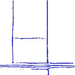
(a) Edelkamp.                     (b) Chen.                     (c) Kharita.      (d) Cao.             (e) Biagioni.         (f) DeepMG.

                                       Figure 5: Seven algorithm at a roundabout near Gongzhufen area in TaxiBJ.

            Edelkamp       Kharita              1.0                                    encoded information. The encoding block and decoding
     1.0    Cao            DeepMG-nt            0.9
                                                       Edelkamp
                                                       Cao
                                                                      Kharita
                                                                      DeepMG-nt
            Biagioni
            Chen
                           DeepMG
                                                0.8    Biagioni       DeepMG           block have linked shortcuts at corresponding layers.
     0.8                                        0.7
                                                       Chen

     0.6                                        0.6                                  • D-LinkNet (Zhou, Zhang, and Wu 2018): D-LinkNet is
F1

                                           F1

                                                0.5                                    a variant of LinkNet, which introduces a bottleneck layer
     0.4                                        0.4
                                                0.3                                    with dilated convolution between encoder and decoder.
     0.2                                        0.2
                                                0.1                                  • LinkNet+1D Decoder (Sun et al. 2019): It is also a variant
           6 8 10 12 14 16 18 20                      6 8 10 12 14 16 18 20            of LinkNet, which replaces the traditional 2D filters of
                       S Res. (m)                                 S Res. (m)
                                                                                       convolution layers in the decoder block with 1D. It is the
              (a) TaxiBJ.                                (b) TaxiJN.                   SOTA method for aerial image segmentation.
                          Figure 6: Performance on F1.                                  We report the average pixel-wise Precision, Recall, and
                                                                                     F1 of the test set in Tab 2. The performance of FCN is the
                                                                                     worst in both two datasets since it predicts results by directly
                                                                                     upsampling from a very small feature map, which makes
for map reconstruction. The corresponding trajectories and                           the location information hard to reconstruct. DeepLabV3+
the ground truth map is already shown in Fig 1. The results                          also doesn’t perform very well, due to there is few informa-
demonstrate that Biagioni, which is a KDE-based method,                              tion fusion between encoder and decoder. Other models fol-
generates few redundant edges, and is robust to the sampling                         lowing the encoder-decoder structure with skip-connections,
rate. However, it is difficult to distinguish two parallel roads.                    shows relatively good performance. Experiments show that
Although the direction is considered in other baselines, it is                       concatenation-based fusion (e.g., UNet) is more effective
difficult to set global consistent parameters, which makes                           than summation-based fusion (e.g., LinkNet and its vari-
the edges too complicated. As shown in the figure, DeepMG                            ants) for centerline inference, since the summation is usually
significantly outperforms baselines, which can successfully                          inaccurate. T2RNet consistently outperforms all alternative
identify parallel roads in the same direction without gener-                         models. An auxiliary task, i.e., road region inference, is in-
ating many redundant edges.                                                          troduced in T2RNet, so that the centerline decoder can fuse
                                                                                     both the encoder and road region decoder information, and
Geometry Translation Component                                                       make more accurate predictions.
Model Comparison. To evaluate the effectiveness of                                   Effect of Multi-task Learning. To show the effectiveness of
T2RNet, we replace the encoder-decoder part of T2RNet                                multi-task learning, we evaluate our model under different λ
with 6 models to directly predict road centerlines.                                  settings from 0 to 0.8. A small λ pays more attention to the
                                                                                     centerline inference task, and a larger λ cares more about
• FCN (Long, Shelhamer, and Darrell 2015): FCN replaces                              road region prediction. The result is shown in Fig 7. We find
  the FC layers of classification nets with convolutions, and                        that when λ = 0.2, T2RNet achieves the best performance
  multi-resolution features are combined before prediction.                          on both two datasets. A smaller λ or a larger λ decreases the
• LinkNet (Chaurasia and Culurciello 2017): LinkNet uses                             centerline inference performance.
  ResNet (He et al. 2016) as the encoder block, and the fea-                         Effect of Different Features. The evaluation of different
  ture maps from the encoder are summed with the upsam-                              feature combinations is shown in Tab 3, where P, L, S,
  pled feature maps from the decoder.                                                A means point feature, line feature, spatial view features,
                                                                                     and all features, respectively. Comparing P and L, we find
• DeepLabV3+ (Chen et al. 2017): DeepLabV3+ encodes
                                                                                     point feature has higher precision than line feature in both
  multi-scale contextual information by applying atrous
                                                                                     datasets, which is consistent with our common knowledge.
  convolution at multiple scales, and then decodes the seg-
                                                                                     However, line feature has a higher recall than point feature
  mentation results along object boundaries.
                                                                                     since it fills the distance gap between consecutive points. We
• UNet (Ronneberger, Fischer, and Brox 2015): UNet con-                              also find that line feature ultimately has a higher F1 score
  sists of an encoding block which downsamples the orig-                             than point feature in TaxiJN, while TaxiBJ is on the opposite.
  inal image, and a decoding block, which upsamples the                              The sampling rate of TaxiJN is much higher than TaxiBJ,
Table 2: Model Comparisons on Different Datasets
TaxiBJ TaxiJN
Methods #Params
Precision Recall F1 Precision Recall F1
FCN 134.3M 0.1824 0.6269 0.2778 0.0255 0.5026 0.0482
LinkNet 21.7M 0.2652 0.4690 0.3325 0.1566 0.3238 0.2059
DeepLabV3+ 50.5M 0.2199 0.5571 0.3107 0.1383 0.3471 0.1883
UNet 39.4M 0.2745 0.4760 0.3439 0.1749 0.2945 0.2079
D-LinkNet 31.1M 0.2637 0.4884 0.3387 0.1654 0.3116 0.2084
LinkNet+1D Decoder 21.8M 0.2576 0.5105 0.3384 0.1602 0.3248 0.2042
T2RNet 63.0M 0.2879 0.5245 0.3678 0.1795 0.3020 0.2156
0.40 0.230
0.38 0.225
0.220
0.36
0.215
F1
F1
0.34
0.210
0.32 0.205 (a) α=1.0 (b) α=1.4 (c) α=3.0
0.30 0.200
0.0 0.2 0.4 0.6 0.8 0.0 0.2 0.4 0.6 0.8
Figure 8: Effect of α.
(a) TaxiBJ. (b) TaxiJN.
Figure 7: Effect of λ. Related Work
Map Reconstruction from Trajectories
Map reconstruction from trajectories is a field that has been
so the line between two consecutive points is highly likely extensively studied for a long time, and the main research
still on the road while this assumption is not held in TaxiBJ. focus is on how to reduce GPS noises and uncertainties. A
Comparing S and A, we demonstrate the effectiveness of the survey is given in (Biagioni and Eriksson 2012a), which cat-
transition view. The improvement of the transition view is egorized existing works into 3 types: 1) Clustering-based
much bigger in TaxiBJ than TaxiJN. This could because fea- method (Edelkamp and Schrödl 2003; Chen et al. 2016;
tures in spatial view are already accurate enough when the Stanojevic et al. 2018) , which firstly identifies nodes (or
sampling rate is high, while the transition view brings more short edges) from raw GPS points using spatial clustering
information gains for low sampling rate trajectories. algorithms based on location closeness and direction simi-
larity, and then links those nodes (or short edges) using tra-
Table 3: Effect of Different Features. jectories; 2) trace-merging based method (Cao and Krumm
2009; Niehöfer et al. 2009), which directly merges edges
TaxiBJ TaxiJN from every consecutive points in trajectories; 3) KDE based
F
Preci. Recall F1 Preci. Recall F1 method (Biagioni and Eriksson 2012b; Wang, Wang, and Li
P 0.2549 0.4840 0.3305 0.1619 0.2966 0.2030 2015) , which performs kernel density estimation over raw
L 0.2293 0.5000 0.3097 0.1580 0.3364 0.2096 GPS points, and several image processing techniques (e.g.,
S 0.2594 0.5196 0.3434 0.1753 0.2893 0.2123 morphological dilation, closing, thinning) are applied to ex-
A 0.2879 0.5245 0.3678 0.1795 0.3020 0.2156 tract road centerlines. However, all existing methods either
cannot handle low sampling rate trajectories or are not able
to identify spatially near parallel roads. In this work, we use
a deep learning-based approach to learn how to reduce noise
Topology Construction Component and detect centerlines, and the connectivity is further refined
We have already quantitatively evaluated the effectiveness of using trajectories.
topology construction in Fig 6. In this subsection, we further
demonstrate a qualitative result. The generated maps under Road Detection from Aerial Images
different α settings are given the Fig 8. The blue lines are the Road detection from aerial images is an active field in the
predicted edges, and the red lines are the links we generated. computer vision community, which essentially corresponds
On one hand, if we do not add a penalty to the generated to a semantic segmentation problem. With the rising of deep
link (α = 1.0), there are many shortcuts generated. On the learning, (Mnih and Hinton 2012; Mnih 2013) employ con-
other hand, if α is too large (e.g., α = 3.0), road segments volutional networks to classify each pixel from a larger
can be broken due to the map matching algorithm has fewer image patch. Due to the performance issues and compli-
chances to match trajectories on those links. Therefore, we cated dependencies with neighborhood locations, predict-
choose α = 1.4, which has a good balance. ing all pixels at once becomes more popular recently, e.g.,Fully Convolutional Network (Long, Shelhamer, and Dar- Edelkamp, S., and Schrödl, S. 2003. Route planning and map
rell 2015), U-Net (Ronneberger, Fischer, and Brox 2015), inference with global positioning traces. In Computer science in
and DeepLab (Chen et al. 2017). CasNet (Cheng et al. 2017) perspective. Springer. 128–151.
uses a cascaded network to extract road region and road cen- He, K.; Zhang, X.; Ren, S.; and Sun, J. 2016. Deep residual learn-
terline from aerial images. D-LinkNet (Zhou, Zhang, and ing for image recognition. In CVPR, 770–778.
Wu 2018) won top places in recent aerial image segmen- Ioffe, S., and Szegedy, C. 2015. Batch normalization: Accelerating
tation challenge (Demir et al. 2018). The closest work to us deep network training by reducing internal covariate shift. arXiv
is (Sun et al. 2019), which leverages both satellite images preprint arXiv:1502.03167.
and GPS trajectories to detect road regions. Instead of treat- Kingma, D. P., and Ba, J. 2014. Adam: A method for stochastic
ing trajectory only from spatial view in (Sun et al. 2019), we optimization. arXiv preprint arXiv:1412.6980.
introduce another transition view to improve the prediction Long, J.; Shelhamer, E.; and Darrell, T. 2015. Fully convolutional
quality. Moreover, most aforementioned works are mainly networks for semantic segmentation. In CVPR, 3431–3440.
focused on detecting road regions from remote sensing data, Máttyus, G.; Luo, W.; and Urtasun, R. 2017. Deeproadmapper:
while we focus on the road centerline inference from trajec- Extracting road topology from aerial images. In ICCV, 3438–3446.
tories, and reconstructing a routable and directed map. Mikolov, T.; Sutskever, I.; Chen, K.; Corrado, G. S.; and Dean, J.
2013. Distributed representations of words and phrases and their
Conclusion compositionality. In NIPS, 3111–3119.
In this paper, we study the problem of generating maps from Milletari, F.; Navab, N.; and Ahmadi, S.-A. 2016. V-net: Fully
trajectories. We propose a deep learning-based map genera- convolutional neural networks for volumetric medical image seg-
tion framework DeepMG. DeepMG can handle trajectories mentation. In 3DV, 565–571. IEEE.
with different sampling rates and distinguish parallel roads Mnih, V., and Hinton, G. E. 2012. Learning to label aerial images
that are spatially close without empirical parameter tuning. from noisy data. In ICML, 567–574.
Experiments on two real-world datasets show DeepMG out- Mnih, V. 2013. Machine learning for aerial image labeling. Cite-
performs baselines by at least 32.3% for low sampling rate seer.
trajectories and 6.5% for high sampling rate trajectories. Niehöfer, B.; Burda, R.; Wietfeld, C.; Bauer, F.; and Lueert, O.
2009. Gps community map generation for enhanced routing meth-
Acknowledgments ods based on trace-collection by mobile phones. In SPACOMM,
156–161. IEEE.
This work was supported by the NSFC Grant No. 61672399,
No. U1609217, and National Key R&D Program of China Ronneberger, O.; Fischer, P.; and Brox, T. 2015. U-net: Convolu-
tional networks for biomedical image segmentation. In MICCAI,
(2019YFB2101800). The research of Cheng Long was sup-
234–241. Springer.
ported by the NTU Start-Up Grant and Singapore MOE Tier
1 Grant RG20/19 (S). Shi, W.; Shen, S.; and Liu, Y. 2009. Automatic generation of road
network map from massive gps, vehicle trajectories. In ITSC, 1–6.
IEEE.
References
Stanojevic, R.; Abbar, S.; Thirumuruganathan, S.; Chawla, S.; Fi-
Biagioni, J., and Eriksson, J. 2012a. Inferring road maps from lali, F.; and Aleimat, A. 2018. Robust road map inference through
global positioning system traces: Survey and comparative evalua- network alignment of trajectories. In ICDM, 135–143. SIAM.
tion. TRANSPORT RES REC 2291(1):61–71.
Sun, T.; Chen, Z.; Yang, W.; and Wang, Y. 2018. Stacked u-nets
Biagioni, J., and Eriksson, J. 2012b. Map inference in the face of with multi-output for road extraction. In CVPR Workshops, 202–
noise and disparity. In SIGSPATIAL, 79–88. ACM. 206.
Cao, L., and Krumm, J. 2009. From gps traces to a routable road
Sun, T.; Di, Z.; Che, P.; Liu, C.; and Wang, Y. 2019. Leveraging
map. In SIGSPATIAL, 3–12. ACM.
crowdsourced gps data for road extraction from aerial imagery. In
Chaurasia, A., and Culurciello, E. 2017. Linknet: Exploiting en- CVPR, 7509–7518.
coder representations for efficient semantic segmentation. In VCIP,
Wang, S.; Wang, Y.; and Li, Y. 2015. Efficient map reconstruction
1–4. IEEE.
and augmentation via topological methods. In SIGSPATIAL, 25.
Chen, C.; Lu, C.; Huang, Q.; Yang, Q.; Gunopulos, D.; and Guibas, ACM.
L. 2016. City-scale map creation and updating using gps collec-
Yuan, J.; Zheng, Y.; Zhang, C.; Xie, W.; Xie, X.; Sun, G.; and
tions. In SIGKDD, 1465–1474. ACM.
Huang, Y. 2010a. T-drive: driving directions based on taxi tra-
Chen, L.-C.; Papandreou, G.; Kokkinos, I.; Murphy, K.; and Yuille, jectories. In SIGSPATIAL, 99–108. ACM.
A. L. 2017. Deeplab: Semantic image segmentation with deep
Yuan, J.; Zheng, Y.; Zhang, C.; Xie, X.; and Sun, G.-Z. 2010b. An
convolutional nets, atrous convolution, and fully connected crfs.
interactive-voting based map matching algorithm. In MDM, 43–52.
TPAMI 40(4):834–848.
IEEE Computer Society.
Cheng, G.; Wang, Y.; Xu, S.; Wang, H.; Xiang, S.; and Pan,
Zheng, Y.; Capra, L.; Wolfson, O.; and Yang, H. 2014. Urban com-
C. 2017. Automatic road detection and centerline extraction
puting: concepts, methodologies, and applications. TIST 5(3):38.
via cascaded end-to-end convolutional neural network. TGRS
55(6):3322–3337. Zheng, Y. 2015. Trajectory data mining: an overview. TIST 6(3):29.
Demir, I.; Koperski, K.; Lindenbaum, D.; Pang, G.; Huang, J.; Zhou, L.; Zhang, C.; and Wu, M. 2018. D-linknet: Linknet
Basu, S.; Hughes, F.; Tuia, D.; and Raska, R. 2018. Deepglobe with pretrained encoder and dilated convolution for high resolution
2018: A challenge to parse the earth through satellite images. In satellite imagery road extraction. In CVPR Workshops, 182–186.
CVPRW, 172–17209. IEEE.You can also read