Magnetically regulated fragmentation of a massive, dense, and turbulent clump
←
→
Page content transcription
If your browser does not render page correctly, please read the page content below
A&A 593, L14 (2016)
DOI: 10.1051/0004-6361/201629442                                                                                    Astronomy
c ESO 2016                                                                                                           &
                                                                                                                    Astrophysics
                                                        Letter to the Editor

          Magnetically regulated fragmentation of a massive, dense,
                             and turbulent clump
 F. Fontani1 , B. Commerçon2 , A. Giannetti3 , M. T. Beltrán1 , A. Sánchez-Monge4 , L. Testi1, 5, 6 , J. Brand7 , P. Caselli8 ,
              R. Cesaroni1 , R. Dodson9 , S. Longmore10 , M. Rioja9, 11, 12 , J. C. Tan13 , and C. M. Walmsley1

      1
          INAF–Osservatorio Astrofisico di Arcetri, Largo E. Fermi 5, 50125 Florence, Italy
          e-mail: fontani@arcetri.astro.it
      2
          École Normale Supérieure de Lyon, CRAL, UMR CNRS 5574, Université Lyon I, 46 allée d’Italie, 69364 Lyon Cedex 07, France
      3
          Max-Planck-Institut für Radioastronomie, auf dem Hügel 69, 53121 Bonn, Germany
      4
          I. Physikalisches Institut, Universität zu Köln, Zülpicher Str. 77, 50937 Köln, Germany
      5
          European Southern Observatory, Karl-Schwarzschild-Str 2, 85748 Garching bei München, Germany
      6
          Gothenburg Center for Advance Studies in Science and Technology, Chalmers University of Technology and University of
          Gothenburg, 412 96 Gothenburg, Sweden
      7
          INAF–Istituto di Radioastronomia and Italian ALMA Regional Centre, via P. Gobetti 101, 40129 Bologna, Italy
      8
          Max-Planck-Institüt für extraterrestrische Physik, Giessenbachstrasse 1, 85748 Garching bei München, Germany
      9
          International Center for Radio Astronomy Research, M468, University of Western Australia, 35, Stirling Hwy, Crawley,
          Western Australia 6009, Australia
     10
          Astrophysics Research Institute, Liverpool John Moores University, Liverpool, L3 5RF, UK
     11
          CSIRO Astronomy and Space Science, 26 Dick Perry Avenue, Kensington WA 6151, Australia
     12
          Observatorio Astronomico Nacional (IGN), Alfonso XII, 3 y 5, 28014 Madrid, Spain
     13
          Departments of Astronomy & Physics, University of Florida, Gainesville, FL 32611, USA

     Received 31 July 2016 / Accepted 27 August 2016

                                                                 ABSTRACT

     Massive stars, multiple stellar systems, and clusters are born of the gravitational collapse of massive, dense, gaseous clumps, and the
     way these systems form strongly depends on how the parent clump fragments into cores during collapse. Numerical simulations show
     that magnetic fields may be the key ingredient in regulating fragmentation. Here we present ALMA observations at ∼0.2500 resolution
     of the thermal dust continuum emission at ∼278 GHz towards a turbulent, dense, and massive clump, IRAS 16061–5048c1, in a very
     early evolutionary stage. The ALMA image shows that the clump has fragmented into many cores along a filamentary structure.
     We find that the number, the total mass, and the spatial distribution of the fragments are consistent with fragmentation dominated
     by a strong magnetic field. Our observations support the theoretical prediction that the magnetic field plays a dominant role in the
     fragmentation process of massive turbulent clumps.
     Key words. stars: formation – submillimeter: ISM – ISM: molecules – ISM: individual objects: IRAS 16061-5048c1

1. Introduction                                                           gravity during collapse are intrinsic turbulence, radiation feed-
                                                                          back, and magnetic pressure (e.g. Krumholz 2006; Hennebelle
High-mass stars, multiple systems, and clusters are born from             et al. 2011). Feedback from nascent protostellar objects through
the gravitational collapse of massive, dense clumps (compact              outflows, winds, and/or expansion of ionised regions (especially
structures with M ≥ 100 M , and n(H2 ) ≥ 104 cm−3 ) inside                from newly born massive objects) can be important in relatively
large molecular clouds. Stars more massive than 8 M are ex-               evolved stages (Bate 2009), but even then seems to be of only
pected to form either through direct accretion of material in             secondary importance (Palau et al. 2013).
massive cores within the clump that does not fragment further                 In a purely gravo-turbulent scenario, the collapsing clump
(e.g. McKee & Tan 2003; Tan et al. 2013), or as a result of               should fragment into many cores, the number of which is com-
a dynamical evolution where several low-mass seeds compet-                parable to the total mass divided by the Jeans mass (Dobbs
itively accrete matter in a highly fragmented clump (Bonnell              et al. 2005); on the other hand, fragmentation can be sup-
et al. 2004). In the latter scenario, each clump forms multiple           pressed by temperature enhancement that is due to the gravi-
massive stars and many lower mass stars: the unlucky losers               tational energy radiated away from the densest portion of the
in the competitive accretion competition. There is still vigor-           clump that collapses first (Krumholz 2006), or by magnetic sup-
ous debate on which of these scenarios is more likely to oc-              port (Hennebelle et al. 2011). Commerçon et al. (2011) have
cur, and fragmentation appears to be particularly important in            shown that models with strong magnetic support predict frag-
this debate. Theoretical models and simulations show that the             ments more massive and less numerous than those predicted by
number, the mass, and the spatial distribution of the fragments           the models with weak magnetic support. The crucial parameter
depend strongly on which of the main competitors of grav-                 in their 3D simulations is µ = (M/Φ)/(M/Φ)crit , where (M/Φ) is
ity is dominant. The main physical mechanisms that oppose                 the ratio between total mass and magnetic flux, and the critical
                                                              Article published by EDP Sciences                                  L14, page 1 of 7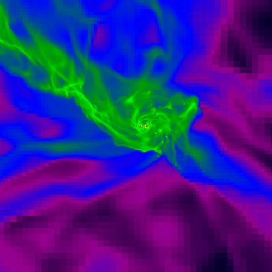
A&A 593, L14 (2016)
value (M/Φ)crit , that is, the ratio at which gravity is balanced
by the magnetic field (thus, for (M/Φ)crit > 1 the magnetic
field cannot prevent gravitational collapse), is given by theory
(Mouschovias & Spitzer 1976). The outcome of the simulations
also depends on other initial global parameters of the clump,
such as gas temperature, angular momentum, total mass, and av-
erage volume density. Once these parameters are fixed, however,
the final population of cores shows a strong variation with µ.
Studies of the fragmentation level in massive clumps at the
earliest stages of the gravitational collapse remain limited so far.
These investigations are challenging for several reasons: pristine,
massive clumps are rare and typically located at distances larger
than 1 kpc, hence reaching the linear resolution required for a
consistent comparison with the simulations (about 1000 AU) re-
quires observations with sub-arcsecond angular resolution. Fur-
thermore, the low mass of the fragments expected in the simula-
tions (fractions of M ) requires extremely high sensitivities. In
general, the few studies performed so far with sub-arcsecond an-
gular resolution, or close to ∼100 , reveal either low fragmentation
(e.g. Palau et al. 2013; Longmore et al. 2011), or many fragments
that are too massive, however, to be consistent with the gravo-
turbulent scenario (Bontemps et al. 2010; Zhang et al. 2015).
Furthermore, comparisons with models that assume the actual
physical conditions (temperature, turbulence) of the collapsing
parent clump have not been published yet.
In this letter, we report on the population of fragments de-
rived in the image of the dust thermal continuum emission at
∼278 GHz obtained with the Atacama Large Millimeter Ar-
ray (ALMA) towards the source IRAS 16061–5048c1, here-
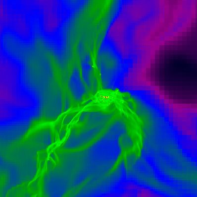
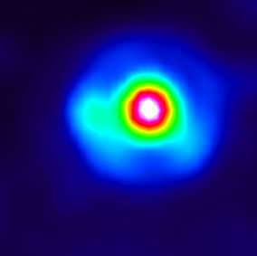
after I16061c1, a massive (M ∼ 280 M , Beltrán et al. 2006; Fig. 1. Panel A): dust continuum emission map (dashed contours) ob-
Giannetti et al. 2013) and dense (column density of H2 , N(H2 ) ∼ tained with the SEST telescope with an angular resolution of 2400 at
1.6 × 1023 cm−2 ) molecular clump located at 3.6 kpc (Fontani 1.2 mm towards I16061c1 (Beltrán et al. 2006). The map is superim-
et al. 2005). The clump was detected at 1.2 mm at low angu- posed on the Spitzer-MIPS image at 24 µm (in units of MJy/sr). The cir-
lar resolution with the Swedish-ESO Submillimeter Telescope cle indicates the ALMA primary beam at 278 GHz (∼2400 ). Panel B): en-
(SEST, panel A of Fig. 1, Beltrán et al. 2006), and found to be largement of the rectangular region indicated in panel A), showing
not blended with nearby millimeter clumps, which allows a clear the contour map of the thermal dust continuum emission at frequency
identification of the fragments. Its high mass and column density 278 GHz detected with ALMA, in flux density units. The first contour
make it a potential site for the formation of massive stars and level and the spacing between two adjacent contours both correspond to
the 3σ rms of the image (0.54 mJy/beam). The cross marks the phase
rich clusters, according to observational findings (Kauffmann & centre. The ellipse in the bottom left corner shows the synthesized beam,
Pillai 2010; Lopez-Sepulcre et al. 2010). The clump was clas- and corresponds to 0.3600 × 0.1800 (Position Angle = 86◦ ). The numbers
sified as an infrared dark cloud because it was undetected in indicate the twelve identified fragments (see Sect. 3). Panel C): simula-
the images of the Midcourse Space Experiment (MSX) infrared tions of the thermal dust emission at 278 GHz predicted by the models
satellite, although more sensitive images of the Spitzer satellite of Commerçon et al. (2011), which reproduce the gravitational collapse
revealed infrared emission at a wavelength of 24 µm (panel A in of a 300 M clump in case of strong magnetic support (µ = 2), ob-
Fig. 1). Nevertheless, several observational results indicate that tained at time t2 (see text), projected on a plane perpendicular to the
the possibly embedded star formation activity is at a very early direction of the magnetic field. Panel D): same as panel C) for the case
stage (Sanchez-Monge et al. 2013). In particular, the depletion µ = 200 (weak magnetic support). Panel E): synthetic ALMA images
factor of CO (ratio between expected and observed abundance of of the models presented in panel C). The contours correspond to 0.54,
1.2, 2, 5, 10, 30, and 50 mJy/beam. Panel F) same as panel E) for the
CO) is 12. This provides strong evidence for the chemical youth case µ = 200 at time t200 (weak magnetic support).
of the clump, because the cause of depletion factors of CO larger
than unity is the freeze-out of this molecule onto dust grains, a
mechanism efficient only in cold and dense pre-stellar and young
protostellar cores (Caselli et al. 1999; Emprechtinger et al. 2009; precipitable water vapour during observations was ∼1.8 mm.
Fontani et al. 2012). The observations and data reduction proce- Bandpass and phases were calibrated by observing J1427−4206
dures are presented in Sect. 2. Our results are shown in Sect. 3 and J1617−5848, respectively. The absolute flux scale was
and discussed in Sect. 4. set through observations of Titan and Ceres. From Beltrán
et al. (2006), we know that the total flux measured with the
2. Observations and data reduction single-dish in an area corresponding to the ALMA primary beam
at the observing frequency (2400 ) is ∼2.3 Jy, while the total
Observations of I16061c1 with the ALMA array were per- flux measured with ALMA in the same area is 0.63 Jy. This
formed during June, 2015. The array was in configuration C36- means that we recover ∼30% of the total flux. The remaining
6, with maximum baseline of 1091 m. The phase centre was ∼70% is likely contained in an extended envelope that is re-
at RA (J2000): 16h 10m 06.00 61 and Dec (J2000): −50◦ 500 2900 . solved out. Continuum was extracted by averaging in frequency
The total integration time on source was ∼18 min. The the line-free channels. The total bandwidth used is ∼1703 MHz.
L14, page 2 of 7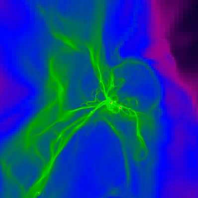
F. Fontani et al.: Magnetically regulated fragmentation

Calibration and imaging was performed with the CASA1 soft-                4. Discussion and conclusion
ware (McMullin et al. 2007), and the final images were analysed
following standard procedures with the software MAPPING of                We have simulated the gravitational collapse of I16061c1
the GILDAS2 package. The angular resolution of the final im-              through 3D numerical simulations following Commerçon
age is ∼0.2500 (i.e. ∼900 AU at the source distance). We were             et al. (2011), adopting a mass, temperature, average density, and
sensitive to point-like fragments of 0.06 M . Together with the           level of turbulence of the parent clump very similar to those
continuum, we detected several lines, among which N2 H+ (3–2).            measured (Beltrán et al. 2006; Giannetti et al. 2013). In partic-
These data will be presented and discussed in a forthcoming pa-           ular, the Mach number setting the initial turbulence was derived
per. In this letter, we only use the N2 H+ (3−2) line to derive the       from the line width of C18 O (3−2) by Fontani et al. (2012). Be-
virial masses, as we show in Sect. 3.                                     cause these observations were obtained with angular resolution
                                                                          of ∼2400 and the critical density of the line (∼5 × 104 cm−3 ,
                                                                          Fontani et al. 2005) is comparable to the average density of the
3. Results                                                                clump as a whole (Beltrán et al. 2006), the C18 O line width rep-
                                                                          resents a reasonable estimate of the intrinsic turbulence of the
The ALMA map of the dust thermal continuum emission is                    parent clump. The models were run for µ = 2 (strongly mag-
shown in Fig. 1B: we have detected several dense condensa-                netised case) and µ = 200 (weakly magnetised case). Then, we
tions distributed in a filamentary-like structure extended east-          post-processed the simulations data and computed the dust emis-
west, surrounded by fainter extended emission. This structure             sion maps at 278 GHz: the final maps obtained in flux density
has been decomposed into twelve fragments (Fig. 1B). The frag-            units at the distance of the source were imaged with the CASA
ments were identified following these criteria: (1) peak intensity        software to reproduce synthetic images with the same observa-
greater than five times the noise level; (2) two partially overlap-       tional parameters as those of the observations. A detailed de-
ping fragments are considered separately if they are separate at          scription of the parameters used for the numerical simulations,
their half-peak intensity level. The minimum threshold of five            of the resulting maps, and how they were post-processed is given
times the noise was adopted because some peaks at the edge                in Appendix B. Further descriptions of the models can also be
of the primary beam are comparable to about four to five times            found in Commerçon et al. (2011). To investigate possible ef-
the noise level. We decided to use these criteria and decompose           fects of geometry, we imaged the outcome of the simulations
the map into cores by eye instead of using decomposition algo-            projected on three planes: (x, y), (x, z), and (y, z), where x is the
rithms (such as Clumpfind) because small changes in their input           direction of the initial magnetic field. As an example, in Figs. 1C
parameters could lead to large changes in the number of identi-           and D we show the results for the cases of strong and weak mag-
fied clumps (Pineda et al. 2009). The main physical properties            netic support, respectively, projected on the (y, z) plane, that is,
of the fragments derived from the continuum map, that is, inte-           on a direction perpendicular to the magnetic field. The synthetic
grated and peak flux, size, and gas mass, and the methods used to         images obtained with CASA are shown in panels E and F. All
derive them, are described in Appendix A. The derived parame-             the planes for µ = 2 and µ = 200 are shown in Appendix B, in
ters are listed in Table A.1. The mean mass of the fragments is           Figs. B.1 and B.2, respectively. An important result of the sim-
4.4 M , with a lowest value of 0.7 M and a highest value of               ulations (see Fig. B.3 in Appendix B) is that the total flux seen
∼9 M . The diameters (undeconvolved for the beam) range from              by the interferometer in the µ = 2 case decreases until about
0.011 to 0.032 pc, with a mean value of 0.025 pc.                         35 × 103 yr and then goes through a minimum and gradually
    To investigate the stability of the fragments, we calculated          starts to increase. In the µ = 200 case, by contrast, the decrease
the virial masses Mvir , that is, the masses required for the cores       is not reversed. We conclude from this that in the µ = 2 case,
to be in virial equilibrium, from the line widths observed in             the fragments continue to accrete material and eventually will
N2 H+ (3−2). As stated in Sect. 2, we here used this molecular            reach the total flux observed in the ALMA image. Thus, in the
transition only for the purpose to derive the level of turbulence         µ = 2 case we analysed the synthetic images produced at the
(the key ingredient of the models, together with the magnetic             time at which the total flux in the fragments matches the ob-
support) of the dense gas out of which the fragments are formed.          served value within an uncertainty of about 10% (the calibration
The approach used to derive Mvir is described in Appendix A               uncertainty on the flux density, see the ALMA Technical Hand-
and the values obtained are reported in Table A.1. The average            book3 ), while for the µ = 200 case we analysed the synthetic
ratio between Mvir and M computed from the continuum emis-                images obtained at the end of the simulations. This corresponds
sion is about 0.4, indicating that the gravity dominates, accord-         to two different times: t2 = 48 500 yr after the birth of the first
ing to other ALMA studies of fragmentation (Zhang et al. 2015).           protostar for µ = 2; t200 = 59 500 yr after the birth of the first
However, the uncertainties due to the dust mass opacity coeffi-           protostar for µ = 200.
cient (see Eq. (A.1)) can be of a factor 2−3, hence it is difficult to        The synthetic maps with µ = 200 show more fragments with
conclude that the fragments are unstable. Moreover, the formula           lower peak fluxes, and the overall structure is more chaotic and
of the virial mass we used does not consider the magnetic sup-            never filamentary, independently of the projection plane. The
port. Because this latter is expected to be relevant, it is likely that   fragments were identified and their properties in the synthetic
the fragments are closer to virial equilibrium and would not tend         images derived following the same criteria and procedures as
to fragment further. If one assumes, for instance, the value of           those used for the ALMA data. Therefore, any systematic error
0.27 mG measured by Pillai et al. (2015) in another infrared-dark         introduced by the assumptions made (e.g. the assumed dust tem-
cloud, the ratio between virial mass and gas mass would become            perature, gas-to-dust ratio, dust grain emissivity) are the same in
about 1, and the fragments would be marginally stable. A similar          the real and synthetic images and consequently do not affect the
conclusion is given in Tan et al. (2013), where the dynamics of           comparison. The statistical properties of the synthetic core pop-
four infrared-dark clouds similar to I16061c1 is studied.                 ulations are summarised in Table B.1 of Appendix B. We also
1
                                                                          compared the cumulative distribution of the peak fluxes of the
  The Common Astronomy Software Applications (CASA) software
can be downloaded at http://casa.nrao.edu                                 3
                                                                            https://almascience.eso.org/proposing/
2
  http://www.iram.fr/IRAMFR/GILDAS                                        technical-handbook

                                                                                                                               L14, page 3 of 7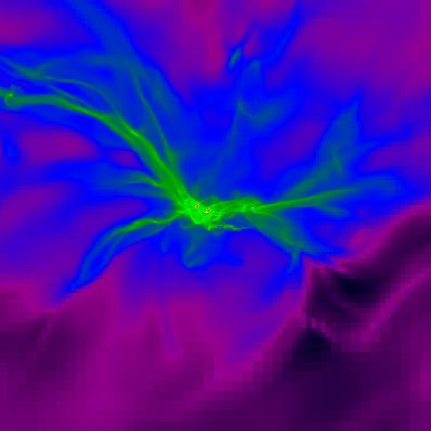
A&A 593, L14 (2016)
6
µ=2
6
µ=200 data clearly is the one with µ = 2. Hence, with these new ALMA
5 5 observations, compared with realistic 3D simulations that as-
4 4
sume as initial conditions the properties of the parent clump, we
demonstrate that the fragmentation due to self-gravity is domi-
N (Fpeak )
N (Fpeak )
3 3 nated by the magnetic support, based on the evidence that (1) the
2 2 overall morphology of the fragmenting region is filamentary, and
this is predicted only in case of a dominant magnetic support;
1 1
(2) the observed fragment mass distribution is most easily un-
0
1.0
0
1.0
derstood in simulations assuming substantial magnetic support.
Acknowledgements. This paper makes use of the following ALMA data:
0.8 0.8
ADS/JAO.ALMA.2012.1.00366.S. ALMA is a partnership of ESO (represent-
ECDF (N < Fpeak )
ECDF (N < Fpeak )
ing its member states), NSF (USA) and NINS (Japan), together with NRC
0.6 0.6
(Canada), NSC and ASIAA (Taiwan), and KASI (Republic of Korea), in co-
operation with the Republic of Chile. The Joint ALMA Observatory is operated
0.4 0.4 by ESO, AUI/NRAO and NAOJ We acknowledge the Italian-ARC node for their
help in the reduction of the data. We acknowledge partial support from Italian
0.2 0.2 Ministero dell’Istruzione, Università e Ricerca through the grant Progetti Premi-
ali 2012 − iALMA (CUP C52I13000140001) and from Gothenburg Centre of
0.0 0.0 Advanced Studies in Science and Technology through the program Origins of
−3.5 −3.0 −2.5 −2.0 −1.5 −1.0 −0.5 −3.5 −3.0 −2.5 −2.0 −1.5 −1.0 −0.5
Log10(Fpeak ) Log10(Fpeak ) habitable planets.
Fig. 2. Top panels: histograms showing the distribution of the peak
fluxes (Fpeak ) of the fragments identified in the ALMA image of
I16061c1 (black), and in the synthetic images for µ = 2 (green, left) References
and µ = 200 (blue, right). Bottom panels: empirical cumulative distri- Bate, M. R. 2009, MNRAS, 392, 1363
bution function (ECDF) of the quantities plotted in the top panels. The Beltrán, M. T., Brand, J., Cesaroni, R., et al. 2006, A&A, 447, 221
black line corresponds to the ALMA data; the green and blue lines in- Beuther, H., Schilke, P., Sridharan, T. K., et al. 2002, A&A, 566, 945
dicate the strong and weak field cases, respectively, projected on the Bleuler, A., & Teyssier, R. 2014, MNRAS, 445, 4015
three planes. In all panels, the different line style indicates the projec- Bonnell, I. A., Vine, S. G., & Bate M. R. 2004, MNRAS, 349, 735
tion plane: solid = (x, y); dot-dashed = (x, z); dashed = (y, z). The Bontemps, S., Motte, F., Csengeri, T., & Schneider, N. 2010, A&A, 524, A18
vertical dotted line corresponds to 0.8 mJy, which is approximately five Caselli, P., Walmsley, C. M., Tafalla, M., Dore, L., & Myers, P. 1999, ApJ, 523,
times the rms noise level in both the real and synthetic maps. Note that L165
Commerçon, B., Hennebelle, P., & Henning, T. 2011, ApJ, 742, L9
the µ = 2 model spans the observations, while the µ = 200 model
Commerçon, B., Launhardt, R., Dullemond, C., & Henning, Th. 2012, A&A,
is strongly biased towards fragments with masses lower than those 545, A98
observed. Commerçon, B., Debout, V., & Teyssier, R. 2014, A&A, 563, A11
Crutcher, R. M. 2013, ARA&A, 50, 29
Dobbs, C. L., Bonnell, I. A., & Clark, P. C. 2005, MNRAS, 360, 2
fragments in the observed and synthetic images. The results are Emprechtinger, M., Caselli, P., Volgenau, N. H., Stutzki, J., & Wiedner, M.C.
shown in Fig. 2. The case with µ = 200 has lower peak values 2009, A&A, 493, 89
for the whole populations, while one or two fragments have a Fontani, F., Beltrán, M. T., Brand, J., et al. 2005, A&A, 432, 921
Fontani, F., Giannetti, A., Beltrán, M. T., et al. 2012, MNRAS, 423, 2342
higher peak value than the maximum observed. The µ = 2 case Fromang, S., Hennebelle, P., & Teyssier, R. 2006, A&A, 457, 371
has a broader distribution of values. Overall, the ALMA map Giannetti, A., Brand, J., Sanchez-Monge, Á., et al. 2013, A&A, 556, A16
shows a narrower distribution of peak fluxes, with a deficit of Hennebelle, P., Commerçon, B., Joos, M., et al. 2011, A&A, 528, A72
very weak and very strong peaks, which in turn are present in Kauffmann, J., & Pillai, T. 2010, ApJ, 723, L7
the two synthetic images. However, the µ = 2 model roughly Krumholz, M. R. 2006, ApJ, 641, L45
Krumholz, M. R., Klein, R., McKee, C. F., Offner, S. S. R., & Cunningham,
spans the observations, while the µ = 200 model is heavily bi- A. J. A. 2009, Science, 323, 754
ased below the data. In addition, a non-parametric statistical test Longmore, S. N., Pillai, T., Keto, E., Zhang, Q., & Qiu, K. 2011, ApJ, 726, L97
(Anderson-Darling test) implies that all the µ = 200 cases can Lopez-Sepulcre, A., Cesaroni, R., & Walmsley, C. M. 2010, A&A, 517, A66
be excluded as being drawn from the same parent distribution Maret, S., Hily-Blant, P., Pety, J., Bardeau, S., & Reynier, E. 2011, A&A, 526,
A47
as the observed values with a confidence level exceeding 99.8%. McKee, C., & Tan, J. C. 2003, ApJ, 585, 850
The µ = 2 case is less obvious because two projections could be McMullin, J. P., Waters, B., Schiebel, D., Young, W., & Golap, K. 2007, in
excluded at a 98−99% confidence level, while the third projec- Astronomical Data Analysis Software and Systems XVI, eds. R. A. Shaw,
tion, (y, z), with a null hypothesis probability of ∼90% cannot F. Hill, & D. J. Bell, ASP Conf. Ser., 376, 127
be excluded at the 2σ level. The deficit of very strong and very Mouschovias, T. C., & Spitzer, L. J. 1976 , ApJ, 210, 326
Ossenkopf, V., & Henning, T. 1994, A&A, 291, 943
weak peaks in the real image may be due to a difference between Palau, A., Fuente, A., Girart, J. M., et al. 2013, ApJ, 762, 120
the µ values assumed in the simulations and the real one, or to Pillai, T., Kauffmann, J., Tan, J. C., et al. 2015, ApJ, 799, 74
some other unknown (or doubtful) initial assumption such as the Pineda, J. E., Rosolowsky, E. W., & Goodman, A. A. 2009, ApJ, 699, L134
density profile or the homogeneous temperature of the collaps- Sanchez-Monge, Á, Beltrán, M. T., Cesaroni, et al. 2013, A&A, 550, A21
Tan, J. C., Kong, S., Butler, M. J., Caselli, P., & Fontani, F. 2013, ApJ, 779, 96
ing clump. Teyssier, R. 2002, A&A, 385, 337
Weiss, A., Hillebrandt, W., Thomas, H.-C., & Ritter, H. 2005, Book review:
Based on the overall morphologies shown in Fig. 1 (and Cox and Giuli’s Principles of Stellar Structure (Cambridge, UK: Princeton
in Figs. B.1 and B.2) and on the statistical properties of the Publishing Associates Ltd)
fragments reported in Fig. 2, the model that better reproduces the Zhang, Q., Wang, K., Xing, L., & Jiménez-Serra, I. 2015, ApJ, 804, 141
L14, page 4 of 7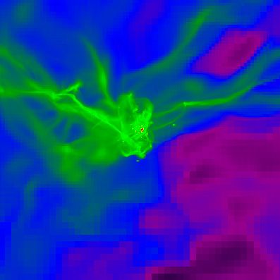
F. Fontani et al.: Magnetically regulated fragmentation

Table A.1. Peak position (in RA and Dec J2000), integrated flux (inside the 3σ rms contour level), peak flux, diameter, mass, line width at half
maximum, and virial mass of the 12 fragments identified in Fig. 1B.

                                                                                 peak
                   Fragment      RA (J2000)      Dec (J2000)       Sν          Sν            D         M       ∆v      Mvir
                                    h:m:s          deg:0 :00        Jy      Jy beam−1        pc       M      km s−1    M
                   1             16:10:07.12     −50:50:27.7      0.007       0.0054       0.011      0.72    0.51     0.28
                   2             16:10:06.93     −50:50:24.4      0.045       0.0092       0.031      4.70    0.90     1.86
                   3             16:10:06.83     −50:50:25.6      0.012       0.0041       0.018      1.25    0.48     0.47
                   4             16:10:06.60     −50:50:26.6      0.012       0.0058       0.016      1.25    0.82     1.26
                   5             16:10:06.40     −50:50:26.0      0.044       0.0048       0.029      4.59    0.49     0.77
                   6             16:10:06.29     −50:50:26.5      0.073       0.0086       0.028      7.62    0.36     0.38
                   7             16:10:06.27     −50:50:27.1      0.050       0.0083       0.023      5.22    0.33     0.26
                   8             16:10:06.16     −50:50:27.3      0.052       0.0180       0.024      5.42    0.84     2.01
                   9             16:10:05.98     −50:50:26.8      0.045        0.010       0.029      4.70    0.33     0.33
                   10            16:10:06.05     −50:50:28.4      0.084        0.011       0.031      8.76    1.04     3.47
                   11            16:10:05.82     −50:50:27.9      0.052       0.0028       0.032      5.43    1.00     3.29
                   12            16:10:05.53     −50:50:30.0      0.032       0.0041       0.030      3.34    0.76     1.82
Notes. The line widths are computed from the N2 H+ (3−2) spectra extracted from the polygons defining the external profile of each fragment, as
explained in Appendix A.

Appendix A: Physical properties of the fragments                             where r is the size of the fragment, and ∆v is the line width at
A.1. Derivation of the parameters                                            half maximum of the average N2 H+ (3–2) spectrum obtained
                                                                             from the fitting procedure described above. The results are
 – Integrated flux densities: the integrated flux densities of the           shown in Table A.1.
   fragments, S ν , were obtained from the 3σ rms contour in
   the continuum image. In the few cases for which the 3σ rms
   contours of two adjacent fragments are partly overlapping
   (e.g. fragments 5, 6, and 7 in Fig. 1), the edges between              Appendix B: Simulations and synthetic images
   the two have been defined by eye at approximately half of
                                                                          B.1. Methods and initial conditions for the numerical
   the separation between the peaks. The results are shown in
                                                                             calculations
   Table A.1.
 – Gas masses: the gas mass of each fragment was calculated               We performed a set of two radiation-magneto-hydrodynamics
   from the equation                                                      calculations that includes the radiative feedback from the
           gS ν d2                                                        accreting protostars. We used the RAMSES code with the
    M=                 ,                                       (A.1)      grey flux-limited-diffusion approximation for radiative trans-
          κν Bν (T d )
                                                                          fer and the ideal magnetohydrodynamics (MHD) for magnetic
   where S ν is the integrated flux density, d is the distance to the     fields (Commerçon et al. 2012, 2014; Teyssier 2002; Fromang
   source, κν is the dust mass opacity coefficient, g is the gas-         et al. 2006). The initial conditions are similar to those used in
   to-dust ratio (assumed to be 100), and Bν (T d ) is the Planck         Hennebelle et al. (2011) and Commerçon et al. (2011), with
   function for a black body of temperature T d . We adopted              slight modifications to match roughly the observed properties
   T d = 25 K, corresponding to the gas temperature derived               of I16061c1. We note that the models presented in this Letter
   by Giannetti et al. (2013), assuming coupling between gas              were made with initial conditions very similar to those mea-
   and dust (reasonable assumption at the high average den-               sured from previous observations in I16061c1to perform an ap-
   sity of the clump). The dust mass opacity coefficient was de-          propriate comparison with observations for this specific source.
   rived from the equation κν = κν0 (ν/ν0 )β . We assumed β = 2           Our aim was not to fine-tune the initial conditions such that the
   and κν0 = 0.899 cm−2 gr−1 at ν0 = 230 GHz, according to                models best reproduce the observations. We considered an iso-
   Ossenkopf & Henning (1994). The highest mass derived is                lated spherical core of mass 300 M , radius 0.25 pc, and tem-
   ∼9 M , the lowest is ∼0.7 M (see Table A.1).                           perature 20 K. We assumed a Plummer-like initial density pro-
 – Size: the size of each fragment was estimated as the diameter          file ρ(r) = ρc /(1 + (r/r0 )2 ), with ρc = 3.96 × 105 cm−3 and
   of the circle with an area equivalent to that encompassed by           r0 = 0.085 pc, and a factor 10 for the density contrast between
   the 3σ rms contour level. The results are shown in Table A.1.          the centre and the border of the core. This density profile is
   The ALMA beam size is much smaller than the size of the                suggested by observational findings (Beuther et al. 2002). The
   fragments, so that deconvolution for the beam is irrelevant to         initial magnetic field was aligned with the x-axis and its inten-
   derive the source size.                                                sity was proportional to the column density through the cloud
 – Virial masses: the virial masses were derived in this way:             (Hennebelle et al. 2011). We here investigated two degrees of
   first, we extracted the N2 H+ (3−2) spectra from the 3σ rms            magnetization, µ = 2, which is close to the values 2−3 that
   level of the 12 continuum cores. All the spectra were fitted           are observationally inferred (e.g. Crutcher 2012), and µ = 200,
   in an automatic way using a procedure based on the integra-            which corresponds to a quasi-hydrodynamical case. Last, we ap-
   tion of the python module PyMC and the CLASS extension                 plied an initial internal turbulent velocity field to the cores. The
   WEEDS (Maret et al. 2011). Then, the virial masses, Mvir ,             velocity field was obtained by imposing a Kolmogorov power
   were computed from the formula                                         spectrum with randomly determined phases (i.e. a ratio 2:1 be-
   Mvir = 210r∆v2 M ,                                          (A.2)      tween the solenoidal and the compressive modes). There is no
                                                                                                                               L14, page 5 of 7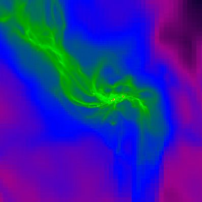
A&A 593, L14 (2016)

global rotation of the cloud, meaning that the angular momen-
tum is contained within the initial turbulent motions, which are
then amplified by the gravitational collapse. The amplitude of
the velocity dispersion was scaled to match a turbulent Mach
number of 6.44, in agreement with C18 O observations (Fontani
et al. 2012). Following Hennebelle et al. (2011, Eq. (2) therein),
the virial parameter was αvir ∼ 0.72 for µ = 2, and αvir ∼ 0.54
for µ = 200 (close to virial equilibrium in both cases). The two
calculations, µ = 2 and µ = 200, started with the same ini-
tial turbulent velocity field (only one realisation was explored)
and turbulence was not maintained during the collapse. Investi-
gation of the effect of different initial turbulent seeds is beyond
the scope of this Letter. The computational box had a 2563 res-
olution, and the grid was refined according to the local Jeans
length (at least 8 cells/Jeans length) down to seven levels of re-
finement (minimum cell size of 13 AU). Below 13 AU, the col-
lapsing gas was described using sub-grid models attached to sink      Fig. B.1. Top panels: show the thermal dust continuum emission
particles, similar to what was done in other studies (Krumholz        map at frequency 278 GHz predicted by the models of Commerçon
et al. 2009). We used the sink particle method presented in           et al. (2011), which reproduce the gravitational collapse of a 300 M
Bleuler et al. (2014), although with slight modifications on the      clump in case of strong magnetic support (µ = 2) at time t2 = 48 500 yr
checks performed for the sink creation. The sink particles accrete    after the birth of the first protostar (see main text for details). In the
the gas that is located in their accretion volumes (sphere of ra-     bottom panels, we show the models after processing in the CASA sim-
dius ∼52 AU, 4 cells) and that is Jeans unstable. We considered       ulator, adopting the same observational conditions as for the real obser-
                                                                      vations. Units of the colour-scale are Jansky/beam. Contour levels are
that half of the mass accreted onto the sink particles becomes        0.6, 1, 5, 10, 30, and 50 mJy beam−1 in all bottom panels.
stellar material. The luminosity of the protostars was then com-
puted using mass-radius and mass-luminosity empirical relations
of main-sequence stars (e.g. Weiss et al. 2005) and was injected
within the accretion volume in the computational domain as a
source term (e.g. Krumholz et al. 2009). We did not account for
accretion luminosity.

B.2. Outcomes of the numerical calculations
We ran the calculations until they reached a star formation effi-
ciency (SFE) > 20% (where the star formation efficiency cor-
responds to the ratio between the mass of the gas accreted onto
the sink particles and the total mass of the cloud). Again, the
choice of the times at which we stopped the calculations was
not aimed at best reproducing the observed values. Model µ = 2
is post-processed at time t2 = 48 500 yr after the birth of the
first protostar, which is the time at which the total flux in frag-
ments is equal to the observed value (within the uncertainty), and
µ = 200 at time t200 = 59 500 yr. At these times, model µ = 2         Fig. B.2. Same as Fig. B.1 for the case µ = 200 at time t200 = 59 500 yr
                                                                      after the birth of the first protostar (see main text for details).
has formed 38 sink particles (for a total mass of 60 M ), while
model µ = 200 has formed 119 sink particles (for a total mass
of 85 M ). Figure B.3 shows the time evolution after the first        stellar irradiation is reprocessed in the envelope at millimeter
sink creation of the SFE, the number of sinks, and the total flux     wavelengths. However, we attempted to create models account-
at 278 GHz (within a total area of 80 000 AU × 80 000 AU) for         ing for protostellar luminosities, and found results that do not
the two models. The circles indicate the time at which the simu-      change significantly at the wavelength considered. The ALMA
lations are post-processed. We note the increase in the 278 GHz       synthetic images of the numerical simulations were then pro-
flux with time for µ = 2, which probably reflects the temperature     duced through the CASA software: first, synthetic visibilities
increase caused by the radiation of the sink particles.               were created with the task simobserve, which were then imaged
                                                                      with the task simanalyze. To precisely reproduce the observa-
B.3. Production of the synthetic images                               tions, we used the same parameters in the tasks as in the obser-
                                                                      vations: integration time on source of 18 min, precipitable water
We first post-processed the RAMSES calculation results using          vapour of about 1.8 mm, array configuration C36-6, start hour
the radiative transfer code RADMC-3D4 and the interface pre-          angle of 2.4 h (see Sect. 2). The population of fragments in the
sented in Commerçon et al. (2012). We produced dust emission          final synthetic images were derived following the same proce-
maps at 278 GHz (see Figs. B.1 and B.2). We did not account           dure as described in Sect. 4.
for the stellar luminosities in the synthetic images since the

4
  http://www.ita.uni-heidelberg.de/dullemond/
software/radmc-3d/

L14, page 6 of 7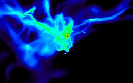
F. Fontani et al.: Magnetically regulated fragmentation

                  120                                                              Table B.1. Statistical comparison between the fragment population de-
                           µ =2                                                    rived from the ALMA image of I16061c1 shown in Fig. 1 and the sim-
                  100
 Number of sink

                           µ =200                                                  ulations presented in Figs. B1 and B2 of the Appendix.
                    80
                    60
                                                                                                         S νtot   M tot   N    Dmean    S νmean   M mean
                    40                                                                                    Jy      M              pc       Jy       M
                    20                                                                 ALMA              0.52     53      12   0.025    0.042     4.42
                     0                                                                 µ = 2 (x, y)      0.36     36      12   0.013    0.026     2.76
                                                                                       µ = 2 (x, z)      0.47     49      12   0.017    0.039      4.1
             0.30                                                                      µ = 2 (y, z)      0.46     42       8   0.018    0.050      5.2
             0.25                                                                      µ = 200 (x, y)    0.22     23      13   0.015    0.017     1.74
                                                                                       µ = 200 (x, z)    0.24     25      15   0.014    0.016     1.67
             0.20                                                                      µ = 200 (y, z)
SFE (%)

                                                                                                         0.28     24      16   0.016    0.021     2.19
             0.15
                                                                                   Notes. The derivation of the parameters obtained for the observed and
             0.10
                                                                                   synthetic images is described in Sect. 3 and in Appendix A, respectively.
             0.05
             0.00

                    2.5

                    2.0
  Total flux (Jy)

                    1.5

                    1.0                                                 (x,y)
                    0.5                                                 (x,z)
                                                                        (y,z)
                    0.0
                       0    10      20    30          40       50       60
                                         Time (kyr)
Fig. B.3. From top to bottom: evolution with time of the number of
sink particles, of the SFE, and of the total flux emission at 278 GHz
(within a total area of 80 000 AU × 80 000 AU) for the two models
after the creation of the first sink. The circles indicate the time at which
the simulations are post-processed. In the bottom panel, the different
lines correspond to the different projection planes as illustrated in the
bottom right corner.

                                                                                                                                           L14, page 7 of 7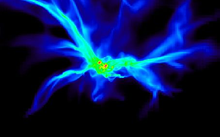
You can also read