Megafauna Aerial Surveys in the Wind Energy Areas of Massachusetts and Rhode Island with Emphasis on Large Whales: Summary Report Campaign 5 ...
←
→
Page content transcription
If your browser does not render page correctly, please read the page content below
OCS Study
                                      BOEM 2021-033

Megafauna Aerial Surveys in the Wind
Energy Areas of Massachusetts and
Rhode Island with Emphasis on Large
Whales: Summary Report Campaign 5,
2018-2019

U.S. Department of the Interior
Bureau of Ocean Energy Management
Office of Renewable Energy Programs
OCS Study
                                                                               BOEM 2021-033

Megafauna Aerial Surveys in the Wind
Energy Areas of Massachusetts and
Rhode Island with Emphasis on Large
Whales: Summary Report Campaign 5,
2018-2019
December 2020

Authors:
Orla O’Brien1, Katherine McKenna1, Brooke Hodge1, Dan Pendleton1, Mark Baumgartner2, and Jessica
Redfern1

Prepared under agreement number M17AC00002.
By
1
  New England Aquarium
Anderson Cabot Center for Ocean Life
1 Central Wharf
Boston MA 02110
2
 Woods Hole Oceanographic Institution
86 Water St
Woods Hole, MA 02543

U.S. Department of the Interior
Bureau of Ocean Energy Management
Office of Renewable Energy Programs
DISCLAIMER
Study collaboration and funding were provided by the US Department of the Interior, Bureau of Ocean
Energy Management (BOEM), Environmental Studies Program, Washington, DC, under Agreement
Number M17AC00002. This report has been technically reviewed by BOEM, and it has been approved
for publication. The views and conclusions contained in this document are those of the authors and should
not be interpreted as representing the opinions or policies of the US Government, nor does mention of
trade names or commercial products constitute endorsement or recommendation for use.

                                   REPORT AVAILABILITY
To download a PDF file of this report, go to the US Department of the Interior, Bureau of Ocean Energy
Management Data and Information Systems webpage (http://www.boem.gov/Environmental-Studies-
EnvData/), click on the link for the Environmental Studies Program Information System (ESPIS), and
search on 2021-033. The report is also available at the National Technical Reports Library at
https://ntrl.ntis.gov/NTRL/.

                                             CITATION
O’Brien, O, McKenna, K, Hodge, B, Pendleton, D, Baumgartner, M, and Redfern, J. 2021. Megafauna
aerial surveys in the wind energy areas of Massachusetts and Rhode Island with emphasis on large
whales: Summary Report Campaign 5, 2018-2019. Sterling (VA): US Department of the Interior, Bureau
of Ocean Energy Management. OCS Study BOEM 2021-033. 83 p.

                                     ABOUT THE COVER
Cover photo taken by NEAq aerial survey team under NOAA permit # 19674.

                                   ACKNOWLEDGMENTS
We would like to extend our thanks to the many people that helped us perform our surveys and conduct
our analyses. First, to Dr. Scott Kraus and Dr. Ester Quintana-Rizzo for their guidance and leadership,
and the aerial observers not involved in the writing of this report. To Dr. Robert Kenney for his timely
and detailed quality control of our data, and answering questions along the way. To Don LeRoi for
continuing to provide input and support on his forward motion compensating camera mount. To the pilots
and staff at AvWatch for their flexibility in providing crew for our surveys. Finally, to the captains and
crew of the R/V Tioga and the F/V Sea Holly for their help in conducting oceanographic analyses.
Contents
List of Figures ................................................................................................................................................iii

List of Tables ................................................................................................................................................. v

List of Abbreviations and Acronyms............................................................................................................. vi

List of Definitions ..........................................................................................................................................vii

1      Introduction ........................................................................................................................................... 1
    1.1        Research objectives ...................................................................................................................... 2

2      Methods ................................................................................................................................................ 2
    2.1        Aerial surveys ................................................................................................................................ 2
       2.1.1           Survey methods for aerial detections .................................................................................... 4
       2.1.2           Sightings: observers and vertical photography ..................................................................... 4
       2.1.3           Right whale photo-identification ............................................................................................ 5
       2.1.4           Sightings per unit effort ......................................................................................................... 5
       2.1.5           Animal density and abundance ............................................................................................. 6
       2.1.6           Sighting rates and temporal variability .................................................................................. 6
       2.1.7           Right whale photographs and demographics........................................................................ 7
    2.2        Oceanographic sampling .............................................................................................................. 7
       2.2.1           Sampling design .................................................................................................................... 7
       2.2.2           In-situ net sampling ............................................................................................................... 8
       2.2.3           In-situ oceanographic observations ...................................................................................... 9
       2.2.4           Analyses .............................................................................................................................. 10

3      Results ................................................................................................................................................ 10
    3.1        Aerial surveys .............................................................................................................................. 10
       3.1.1           Field effort ........................................................................................................................... 10
       3.1.2           Detections ........................................................................................................................... 12
       3.1.3           Cetacean detections ........................................................................................................... 13
       3.1.4           Sperm whales...................................................................................................................... 37
       3.1.5           Sea turtles ........................................................................................................................... 46
       3.1.6           Other marine megafauna .................................................................................................... 48
    3.2        Oceanographic Sampling ............................................................................................................ 49
       3.2.1           In-situ observations ............................................................................................................. 49

4      Discussion ........................................................................................................................................... 55
    4.1        Aerial surveys .............................................................................................................................. 55
       4.1.1           North Atlantic right whales .................................................................................................. 55

                                                                                 i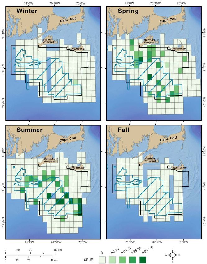
4.1.2         Balaenopterid whales .......................................................................................................... 56
       4.1.3         Small cetaceans .................................................................................................................. 57
       4.1.4         Sea turtles ........................................................................................................................... 57
       4.1.5         Other marine fauna ............................................................................................................. 57
       4.1.6         Conclusion........................................................................................................................... 57
    4.2       Oceanographic Sampling ............................................................................................................ 58

5      References .......................................................................................................................................... 60

Appendix A: Aerial Sightings ....................................................................................................................... 62

Appendix B: Discussion section from Part 1 of report ................................................................................ 70

                                                                              ii
List of Figures
Figure 1. Study area in the offshore waters of Massachusetts and Rhode Island ....................................... 3

Figure 2. NEAq observer taking photographs during a whale sighting ......................................................... 5

Figure 3. Location of four standard oceanographic sampling stations in the study area ............................. 8

Figure 4. Deployment of the conductivity-temperature-depth (CTD) instrument at sea .............................. 9

Figure 5. Percentage of on effort sightings per cetacean species identified during Campaign 5 aerial
surveys ........................................................................................................................................................ 13

Figure 6. Percentage of individuals identified per cetacean species while on effort during Campaign 5
aerial surveys .............................................................................................................................................. 14

Figure 7. Right whale sightings per month during Campaign 5 aerial surveys........................................... 16

Figure 8. Maps of right whale sightings during Campaign 5 aerial surveys ............................................... 17

Figure 9. Seasonal sightings of right whales during all Campaign 5 aerial surveys ................................... 18

Figure 10. Sightings per unit effort for right whales during all Campaign 5 aerial surveys......................... 19

Figure 11. Right whale #4180 and her calf of the year at the surface side by side .................................... 21

Figure 12. Number of individual right whales resighted across different months during Campaign 5 aerial
surveys ........................................................................................................................................................ 21

Figure 13. Sightings of entangled right whale #2310.................................................................................. 22

Figure 14. Fin whale sightings per month during Campaign 5 aerial surveys ............................................ 23

Figure 15. Map of fin whale sightings during Campaign 5 aerial surveys .................................................. 24

Figure 16. Sightings per unit effort for fin whales during all Campaign 5 aerial surveys ............................ 25

Figure 17. Sei whale sightings per month summarized for all sightings during Campaign 5 aerial surveys
.................................................................................................................................................................... 27

Figure 18. Sightings of sei whales during all Campaign 5 aerial surveys ................................................... 27

Figure 19. Sightings per unit effort for sei whales during all Campaign 5 aerial surveys ........................... 28

Figure 20. Minke whale sightings per month during all Campaign 5 aerial surveys ................................... 30

Figure 21. Map of minke whale sightings during Campaign 5 aerial surveys............................................. 31

Figure 22. Sightings per unit effort for minke whales during all Campaign 5 aerial surveys ...................... 32

Figure 23. Humpback whale sightings per month during Campaign 5 aerial surveys ................................ 34

Figure 24. Map of humpback whale sightings during all Campaign 5 aerial surveys ................................. 35

Figure 25. Sightings per unit effort for humpback whales during all Campaign 5 aerial surveys ............... 36

Figure 26. Sightings of sperm whales during all Campaign 5 aerial surveys ............................................. 38

Figure 27. Two sperm whales sighted south of Nantucket on June 12, 2019 ............................................ 39

                                                                                 iii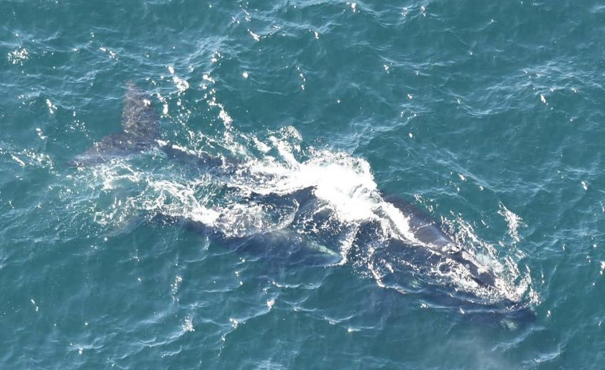
Figure 28. Sightings per month for four species of small cetaceans during all Campaign 5 aerial surveys
.................................................................................................................................................................... 41

Figure 29. Common dolphin sightings per month during all Campaign 5 aerial surveys ........................... 42

Figure 30. Sightings of small cetaceans during all Campaign 5 aerial surveys.......................................... 43

Figure 31. Map of common dolphin sightings during Campaign 5 aerial surveys ...................................... 44

Figure 32. Sightings per unit effort for common dolphins during all Campaign 5 aerial surveys................ 45

Figure 33. Sea turtle sightings per month summarized for all Campaign 5 aerial surveys ........................ 47

Figure 34. Map of sea turtle sightings during all Campaign 5 aerial surveys ............................................. 47

Figure 35. Shark and fish sightings per month during Campaign 5 aerial surveys .................................... 48

Figure 36. Map of shark and fish sightings during all Campaign 5 aerial surveys...................................... 49

Figure 37. Temperature and salinity profiles collected at all stations in 2017 and 2019 ........................... 51

Figure 38. Zooplankton community composition at the four standard stations and at locations near right
whales ......................................................................................................................................................... 53

Figure 39. Interannual comparison of monthly base-10 log-transformed copepod abundance for Calanus
finmarchicus, Centropages spp., and Pseudocalanus spp. ........................................................................ 54

Figure 40. Proportion of developmental stages for Calanus finmarchicus collected during zooplankton
sampling in 2017 (top) and 2019 (bottom) .................................................................................................. 55

                                                                                  iv
List of Tables
Table 1. Standard oceanographic sampling station locations ..................................................................... 7

Table 2. Summary of aerial survey effort during Campaign 5 .................................................................... 11

Table 3. Monthly presence and absence of rorqual whales during Campaign 5 aerial surveys ................ 14

Table 4. Density and abundance of right whales during Campaigns 4 and 5 by season and year ............ 20

Table 5. Number and percentage of different sex and age classes of right whales identified during
Campaign 5 aerial surveys.......................................................................................................................... 20

Table 6. Density and abundance of fin whales during Campaigns 4 and 5 by season and year ............... 26

Table 7. Density and abundance of sei whales Campaigns 4 and 5 by season and year ......................... 29

Table 8. Density and abundance of minke whales during Campaigns 4 and 5 by season and year ......... 33

Table 9. Density and abundance of humpback whales during Campaigns 4 and 5 by season and year .. 37

Table 10. Density and abundance of common dolphins during Campaigns 4 and 5 by season and year . 46

Table 11. Summary of oceanographic surveys during Campaign 5 .......................................................... 50

Table A-1. Summary of all on effort aerial observer and vertical photograph detections of marine
megafauna during Campaign 5 general and condensed aerial surveys .................................................... 62

Table A-2. Summary of all on and off effort aerial observer and vertical photograph detections during
Campaign 5 general and condensed aerial surveys ................................................................................... 63

Table A-3. Summary of all aerial observer and vertical photograph detections during all Campaign 5
directed and opportunistic aerial surveys.................................................................................................... 66

Table A-4. Summary of on and off effort aerial observer and vertical photograph detections during all
Campaign 5 aerial surveys.......................................................................................................................... 67

                                                                          v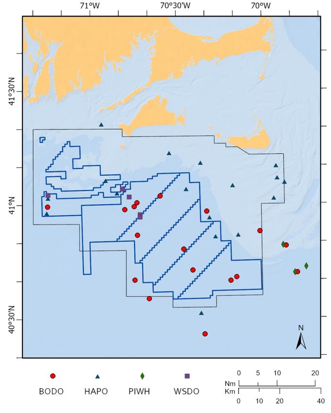
List of Abbreviations and Acronyms

#                   number of vertical photographs
95% CI              95% confidence interval
a                   area sampled (in density calculations)
AIC                 Akaike’s information criterion
BOEM                Bureau of Ocean Energy Management
CCS                 Center for Coastal Studies
cm                  centimeter
CTD                 Conductivity-temperature-depth
d                   density (number of individuals per square kilometer)
ECOMON              Ecosystem Monitoring survey
ESA                 Endangered Species Act
f(0)                probability density function evaluated at zero distance
ft                  feet
G                   number of groups sighted
g                   average group size (in density calculations)
GPS                 global positioning system
h                   hours
I                   number of individuals sighted
km                  kilometer
kts                 knots
L                   length of transect (in density calculations)
m                   meter
ml                  milliliter
mm                  millimeter
MARMAP              Marine Resources Monitoring, Assessment, and Prediction
MassCEC             Massachusetts Clean Energy Center
MAWEA               Massachusetts wind energy area
min                 minutes
NARWC               North Atlantic Right Whale Consortium
N                   estimated abundance
°N                  degrees North
n                   number (of animals/groups sighted during a transect)
nm                  nautical mile
NEAq                New England Aquarium
NEFSC               Northeast Fisheries Science Cente
NOAA                National Oceanic and Atmospheric Administration
RIMA                Rhode Island Massachusetts wind energy area
s                   second
S                   number of sightings
SA                  study area
SPUE                Sightings per unit effort
SR                  Sighting rates
SE                  Standard error
T                   number of transects flown

                                    vi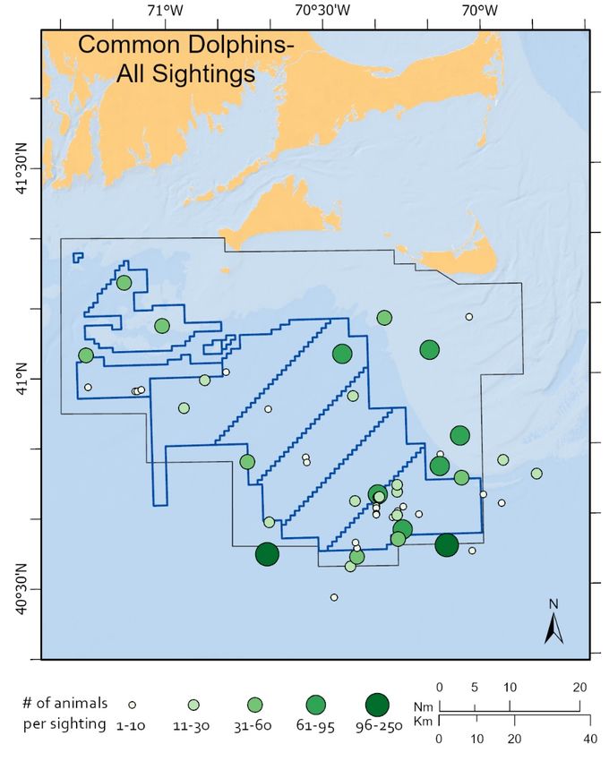
URI                               University of Rhode Island
°W                                degrees West
WEA                               wind energy area
WHOI                              Woods Hole Oceanographic Institution

List of Definitions
Seasons
    •     Winter = December, January, and February
    •     Spring = March, April, and May
    •     Summer = June, July, and August
    •     Fall = September, October, and November

Survey leg stages
   • Transit: travel in the survey area, to the first transect line or from the last transect line
   • Transect: flight along a defined survey line
   • Cross-leg: flight between two transect lines
   • Circling: departure from a transect line to document a sighting

Campaign schedule
   • Campaigns 1-3: October 2011 – June 2015
   • Campaign 4: February 2017 – July 2018
   • Campaign 5: October 2018 – August 2019

                                                      vii
1 Introduction
Beginning in 2013, the Bureau of Ocean and Energy Management (BOEM) designated two wind energy
areas (WEAs) in New England: one offshore of Massachusetts and the other offshore of both Rhode
Island and Massachusetts. Currently, four offshore wind developers have lease agreements to build
projects in the BOEM designated Massachusetts (MA) and the Rhode Island/Massachusetts (RIMA) wind
energy areas. In August 2016, the Governor of Massachusetts, Charles Baker, signed energy diversity
legislation that requires Massachusetts utilities to initiate a procurement of up to 1,600 megawatts of
offshore wind energy by June 30, 2017. The authorized procurement amount was increased to 3,200
megawatts in 2019. As of July 2020, utilities in Massachusetts, Rhode Island, Connecticut and New York
have contracted to purchase the output from over 4,000 megawatts of offshore wind from the WEAs, with
additional procurements planned and in process.
Under the National Environmental Policy Act of 1969 (42 U.S.C. 4371 et seq.), BOEM and other relevant
federal agencies are required to integrate environmental assessments into offshore development and
construction plans. Offshore wind energy planning and development requires comprehensive assessments
of biological resources within suitable development areas to identify and mitigate any potential effects of
that development on marine species.
In anticipation of these requirements, the Massachusetts Clean Energy Center (MassCEC) used a
competitive procurement process in early 2011 to select a team led by the New England Aquarium
(NEAq) to conduct aerial and acoustic surveys of endangered whales and turtles in the MA WEA. Upon
conclusion of these initial surveys (Campaign 1), MassCEC and BOEM extended the surveys for an
additional two years and expanded the geographic scope of the survey area to include the RIMA WEA
(Campaigns 2 and 3). For these three survey campaigns, 76 aerial surveys were conducted between
October 2011 and June 2015.
The final report summarizing Campaigns 1-3, released on October 25, 2016, showed that the study area
included seasonal aggregations of protected species of whales and sea turtles. It also showed that North
Atlantic right whales (Eubalaena glacialis), a critically endangered species, occurred in the study area
during winter and spring, with a peak in March. Based on these findings, the report provided
recommendations for managing geological surveys and construction by scheduling those activities during
off-peak right whale seasons to mitigate or avoid impacts. The 2016 final report also provided
recommendations for additional surveys to address information gaps and for the collection of additional
baseline data.
Acting upon the recommendations in the 2016 final report and with additional funding support from
BOEM, MassCEC contracted with NEAq to conduct additional surveys for the period February 2017
through July 2018 (Campaign 4). A further report summarizing Campaign 4 was released in December
2019. This report showed continued usage of the study area by protected species of whales and sea turtles.
The Campaign 4 report also showed an increase in the number of right whales in the study area and that
right whales occurred in the study area throughout the year. To further understand species distribution
and abundance patterns in the study area, additional aerial surveys using both observer sightings and
automated vertical photography were conducted from October 2018 to August 2019 (Campaign 5, the
subject of this report).
As part of Campaigns 4 and 5 and under sub-contracts to NEAq, the Woods Hole Oceanographic
Institution (WHOI), in coordination with the Provincetown Center for Coastal Studies, conducted
oceanographic surveys to assess the physical and biological characteristics of waters used by right whales
in the study area. Right whales visit the study area annually during winter and spring, but little is known
1about why they come to this region. One hypothesis is that they use the region as a feeding habitat, but
very few zooplankton samples have been collected in the area for the express purpose of determining
right whale prey species and the life history, distribution, and abundance of those prey species. In
response to this knowledge gap, WHOI conducted oceanographic and zooplankton sampling in the
northern region of the study area from February to May 2017 for Campaign 4 and during the winter and
spring of 2019 for Campaign 5.
This report, Summary Report: Campaign 5, 2018-2019, summarizes results from the Campaign 5 surveys
conducted in the study area between October 2018 and August 2019. Specifically, this report includes the
sightings and data information, plus analyses of effort corrected data, and includes maps of sightings per
unit effort (SPUE), sighting rates, and calculations of density and abundance. This report also includes
analysis of right whale prey species and oceanographic conditions near right whale aggregations during
Campaign 4 and 5.
1.1 Research objectives
1. Estimate distribution and relative abundance of large whales (with a focus on right, humpback,
fin, and minke whales) and turtles within the study area, which includes the Massachusetts (MA)
and the Rhode Island/Massachusetts (RIMA) wind energy areas (WEA).
2. Assess prey species and oceanographic conditions near right whale aggregations in the WEA.
2 Methods
2.1 Aerial surveys
During the period of performance between October 2018 and August 2019, four types of aerial surveys
were conducted within the study area. The study area is defined by a polygon surrounding the general and
condensed surveys (shown in Figure 1A).
• General surveys were standardized line-transect surveys that were conducted on a monthly basis
and covered the waters of the study area (5,811 km2), including the MA and RIMA WEA. These
surveys focused on all marine megafauna visible from the plane (excluding birds) and were
comprised of ten north-south tracklines (Figure 1B) evenly spaced at approximately six nautical
miles (nm). Eight survey options are available: each option shifts all 10 tracklines 0.75 nm east or
west, but maintains the six nm spacing between tracklines. One of these options was selected at
random before each survey.
• Condensed surveys were standardized line-transect surveys conducted in two smaller areas off
Martha’s Vineyard and Nantucket. These surveys focused on areas identified by Leiter et al.
(2017) as having high densities of right whales (Figures 1C and 1D) and were compromised of
10-12 tracklines (western side: 10 tracklines, total length: 218 nm; eastern side: 12 tracklines,
total length: 221.5 nm) evenly spaced at three nm. Four survey options are available: each option
shifts all 10-12 tracklines 0.75 nm east or west, but maintains the three nm spacing between
tracklines. One of these options was selected at random before each survey.
• Directed surveys were flown in areas of right whale aggregations, identified by NEFSC or found
during General surveys. These surveys followed line-transect protocols, but the area, number of
lines, and length of flight varied based on the location of the right whale aggregations.
• Opportunistic surveys were flown in response to reports of right whales near shore or to provide
aerial support to oceanographic sampling of right whale aggregations. Opportunistic surveys were
short and did not use planned tracklines.
2Figure 1. Study area in the offshore waters of Massachusetts and Rhode Island
A) Study area (black outline), with the region covered by general surveys depicted by a yellow polygon and regions covered by condensed surveys depicted by a
red (western side) and a green (eastern side) polygon. Examples of tracklines for a B) general survey (tracklines are shown for option 1), C) western survey
(tracklines are shown for option 1), and D) eastern survey (tracklines are shown for option 1). Note: Existing lease areas are depicted in blue.
32.1.1 Survey methods for aerial detections
All surveys were flown in a Cessna Skymaster 337 O-2A at an altitude of 305 m (1,000 ft) and a ground
speed of approximately 185 km/h (100 kts) under Visual Flight Rules. Preferred survey conditions
included winds of ≤10 kts, a Beaufort sea state of ≤ 4, a minimum cloud ceiling of ≥ 2,000 ft, and
visibility ≥ 5 nm. A computer data-logger system (Taylor et al. 2014) automatically recorded flight
parameters (e.g., time, latitude, longitude, heading, altitude, speed) at frequent intervals (every 2–5 sec).
Two experienced aerial observers were positioned aft of each pilot on either side of the aircraft and
scanned the water out to 3.7 km (2 nm) from the transect line.
2.1.2 Sightings: observers and vertical photography
Observers recorded sightings according to the North Atlantic Right Whale Consortium (NARWC)
Database guidelines (Kenney 2010). A sighting is defined as an animal (or group of animals) or object
(fishing gear, vessel, etc.) marked by the plane and could include multiple individuals. Sighting locations
were added to a data log by remote keypads when the detected animal was abeam of the aircraft. The
observer estimated distance from the transect line using calibrated markings on the wing strut (Mbugua
1996, Ridgway 2010). Distances (nm) were binned into the following classes: within ⅛, ⅛ to ¼, ¼ to ½,
½ to 1, 1 to 2, 2 to 4, and >4. The observer also noted whether the sighting occurred on the port or
starboard side of the aircraft. All sightings recorded by observers were integrated into a single datasheet
spanning the entire survey and are listed in a digital survey file.
Sightings, distances, environmental data, and survey parameters were recorded in a digital voice recorder
and transcribed into the data log post-flight. Survey parameters included the four survey leg stages:
transect (flight along a defined survey line); cross-leg (flight between two transect lines); circling
(departure from a transect line to document a sighting); and transit (travel in the survey area, to the first
transect line or from the last transect line). Survey parameters also included transect number and specific
points of a given transect (begin, end, break off, or resume). Environmental data parameters included
general weather conditions (clear, overcast, hazy, etc.), visibility, Beaufort sea state, cloud cover, and sun
glare. Sighting data include species identification to the lowest taxonomic level possible, the reliability of
that identification (definite, probable, possible), a count of individuals in the group, an index of the
precision of that count (+/- 0, 1, 2, 5, 10, and so on), the number of calves, heading of the animal or
group, whether or not photographs were taken, and notes on behaviors.
Observers were unable to see directly under the aircraft. Therefore, a Canon EOS 5D Mark III camera
with a Zeiss-85 mm lens and polarizing filter was fitted in the built-in-camera port of the Cessna O-2A
Skymaster. A forward motion compensation system was used to reduce motion blur. The system was
integrated with a GPS, a Getac E119 Rugged tablet, and observer sighting buttons via a custom data-
logging software (d-Tracker).
Vertical photographs were analyzed by trained observers for detections of marine species, fixed fishing
gear, and debris using the program FastStone Image Viewer. Data recorded for each sighting included
species, identification reliability, and number of individuals with an estimate of the level of confidence in
the count, frame number, time, observer, and area of image. The vertical photograph sighting information
was added to the corresponding event recorded in the survey file by d-Tracker. All detections were
reviewed for accuracy and consistency by another trained expert. Completed data files were submitted to
the NARWC Database.
Distance sampling protocols dictate how sightings data can be incorporated into abundance estimates.
Surveys must have a randomized start point (i.e., a randomly chosen survey option); consequently,
opportunistic and directed survey sightings are not used to estimate abundance. Sightings must be
4observed while on transect; consequently, sightings during transit, cross-leg, or circling are not used to
estimate abundance. Hereafter, on effort refers to sightings that will be used for abundance estimates and
off effort refers to sightings that will not be used for abundance estimates.
Two types of detections are defined: 1) observer detections are sightings marked by observers while in
the plane and 2) camera detections are sightings found in vertical photographs during photo analysis and
are unique from observer detections. All vertical photographs were analyzed for the presence of marine
megafauna during Campaign 5 surveys. On effort photographs were additionally scrutinized for smaller
objects, such as small fish, birds, debris, and fishing gear.
2.1.3 Right whale photo-identification
North Atlantic right whales were a primary target species of the surveys. The rostral callosity pattern and
other obvious scars or markings were used to identify individual right whales. When observers spotted
right whales, the plane deviated from the transect and observers attempted to photograph each whale for
individual identification (Kraus et al. 1986) using a Nikon D500 camera equipped with a 300 mm f/2.8
telephoto lens (1.4×teleconverter; Figure 2). When photographic documentation was complete, the
aircraft returned to the transect at the point of departure for that sighting and resumed the survey.
Figure 2. NEAq observer taking photographs during a whale sighting
2.1.4 Sightings per unit effort
To minimize bias from the uneven allocation of survey effort in both time and space, we calculated the
sightings per unit effort (SPUE). This index of relative density is defined as the number of individuals per
1,000 km of effort and allows comparisons between discrete spatial units. We calculated SPUE in grid
cells measuring 5 min of latitude (9.3 km) by 5 min of longitude (approximately 7 km narrowing slightly
from south to north). The appropriate grid cell size can be determined by weighing the size of the survey
5area against the trackline spacing of the survey. The grid cell size used in this report was also used in
analyses of data collected on Campaign 1-4 surveys funded by MassCEC/BOEM and allows for
comparisons among years. We used all definite and probable sightings in the calculations and transects
flown in the following conditions: altitude ≤ 366 m, visibility ≥ 3.7 km (2 nm), and sea state ≤ 3 (Kraus et
al. 2016).
2.1.5 Animal density and abundance
We estimated density and abundance for baleen whales and common dolphins for Campaigns 4 and 5
following methodology in Buckland et al. (1993). Campaign 4 calculations are included here, rather than
in the Campaign 4 report, because the sample size from the Campaign 4 data alone was too small to
support these analyses. Density is defined as the estimated number of individuals per square kilometer.
Abundance is computed by multiplying the estimated density by the size of the study area, and is defined
as the estimated number of individuals in the study area.
To calculate density, we fit a detection function to our data using the R package Distance (R
Development Core Team, 2018; Miller, 2020). A detection function models the relationship between the
distance of an animal from the trackline and the probability it is detected. This key concept in distance
sampling helps us account for animals that are not seen during a survey. To fit a detection function, it is
necessary to have an adequate sample size: at least 25-30 detections, but ideally 60-80 detections. To
achieve this sample size for low density species such as large cetaceans, species with similar sighting cues
are often pooled. In previous work on this data set, all large whale detections (right, humpback, fin, sei
and sperm whales) were pooled to achieve the sample size necessary to fit detection functions. For this
report, using 2017-2019 data, we were able to fit a unique detection function for right whales and minke
whales, and a pooled detection function for fin, sei and humpback whales. For common dolphins, there
are not enough sightings in the Campaigns 4 and 5 data to fit a detection function, so we used data from
Campaigns 1-5. After fitting several models and truncation distances, we used Akaike’s information
criterion (AIC) scores to choose the best model for each set of species. Having selected the best models,
we were able to use seasonal encounter rates for each species to calculate abundance (Tables 5, 8-12).
An estimate of density (d, in individuals/km2) of a given species was calculated for each survey transect
line by:
n ∙ g ∙ f(0)
d=
2L
where n is the number of groups sighted during the transect, g is the average group size for the species
across all sightings during the study, f(0) is derived from the pooled or unpooled detection function, and L
is the length of the transect (the length is multiplied by two to represent both sides of the trackline).
Average density for the survey area was calculated using the weighted mean density of all survey
transects. Abundance was then calculated by multiplying the density estimates by 5,811 km2 – the size of
the survey area for all flights between 2017-2019. To estimate density, we used sightings with definite or
probable species identification that met the following criteria: collected during general surveys, collected
on tracklines or during circling, altitude ≤ 366 m, visibility ≥ 3.7 km (2 nm), and sea state ≤ 3 (Kraus et
al. 2016). Upper and lower 95% confidence limits for the abundance estimates were calculated using the
weighted average of the variance in encounter rate for all transects flown during each season-year
(Buckland et al. 1993).
2.1.6 Sighting rates and temporal variability
Sighting rates were calculated as the number of individuals divided by the distance traveled on effort.
Sighting rates were multiplied by 1,000 to avoid working with small decimal values and are hereafter
6referred to as animals/km (Kraus et al. 2016, Leiter et al. 2017). Effort was defined as the total distance
flown by the aircraft in km, including transects, transits, cross-legs, and circling when Beaufort sea state
was ≤ 3. Only sightings identified as definite and probable were included in the analysis. Vertical camera
detections were used in the calculations, including animals found in photographs while the plane was
circling.
Seasonal sighting rates were calculated for species with at least 25 sightings. The six species included in
the analysis were right whales, fin whales, sei whales, minke whales, humpback whales, and common
dolphins. Seasons were defined as follows: winter = December, January, and February; spring = March,
April, and May; summer = June, July, and August; and fall = September, October, and November.
2.1.7 Right whale photographs and demographics
Right whale images were uploaded and processed in the NARWC Catalog (Hamilton et al. 2007) and
were compared by observers to catalogued right whales to identify individuals. Once matched,
demographic information such as sex, age, and reproductive status were added to sighting information.
2.2 Oceanographic sampling
2.2.1 Sampling design
Zooplankton and oceanographic sampling occurred at four standard oceanographic stations (Table 1,
Figure 3) as well as at stations adaptively located near North Atlantic right whales. The standard stations
were located in the northern part of the study area to allow our sampling platforms, the F/V Sea Holly and
the R/V Tioga based in Woods Hole, Massachusetts, to visit all of the stations and conduct additional
adaptive sampling in a single day. We chose to sample at four stations distributed in the northern part of
the study area to understand spatial variability in zooplankton distribution.
Table 1. Standard oceanographic sampling station locations
Station Latitude Longitude
1 41 08.8185 N 70 56.6727 W
2 41 01.9200 N 70 42.4440 W
3 41 07.8240 N 70 34.3920 W
4 41 13.7460 N 70 26.2680 W
7Figure 3. Location of four standard oceanographic sampling stations in the study area
Three types of survey trips were used: (1) full sampling trips that allowed sampling at all four standard
stations and if available, sampling at two right whale sampling stations, (2) sampling trip to Station 1 only
(called the Nomans station) and (3) right whale sampling trips that sampled at Station 1 and only at right
whale sampling stations thereafter. Sampling trips were closely coordinated with the NEAq aerial survey
team and the National Oceanic and Atmospheric Administration (NOAA) Northeast Fisheries Science
Center (NEFSC) small boat team, who sometimes accompanied us to sea. Both of these groups were
surveying for right whales and alerted us to the presence of right whales so that we could sample near
them. At each station, a zooplankton sample and oceanographic observations were collected.
2.2.2 In-situ net sampling
Zooplankton net sampling was conducted with a 70-cm ring net outfitted with 333-micron mesh net
hauled obliquely between the surface and the sea floor. A General Oceanics flowmeter was suspended in
the middle of the ring net, and a Seabird SBE39 telemetering temperature-pressure instrument was affixed
to the net tow cable to allow the net to sample close to the sea floor. Collected animals were transferred
from the net cod end to a 333-micron (or smaller) mesh sieve, and then to a 1-liter sample jar. The
sample was preserved with 50 ml of buffered formalin (creating a 5% formalin solution). After the field
season, all samples were sent to the Atlantic Sorting Center at the Huntsman Marine Science Center in
New Brunswick, Canada for identification and enumeration. All copepodid developmental stages of
Calanus finmarchicus (C1-C6) were determined, enumerated, and recorded separately. Taxa abundance
(equivalently concentration) was calculated as the total number of individuals collected divided by the
volume filtered by the net (calculated as the product of the area of the net mouth opening and the distance
traveled by the net as measured by the flowmeter).
82.2.3 In-situ oceanographic observations
Vertical profiles of temperature, conductivity (from which salinity is derived), and chlorophyll
fluorescence were collected at each sampling station with a conductivity-temperature-depth (CTD)
instrument (Figure 4). The instrument was also equipped with a chlorophyll fluorometer, which provides
a relative measure of phytoplankton abundance.
Figure 4. Deployment of the conductivity-temperature-depth (CTD) instrument at sea
WHOI technician Phil Alatalo prepares to deploy the instrument package containing the conductivity-temperature-
depth (CTD) instrument from the stern of the F/V Sea Holly on a delightfully calm day at sea in February 2019.
92.2.4 Analyses
We used the in-situ observations from 2017 (Campaign 4) and 2019 (Campaign 5) to characterize both
oceanographic conditions and zooplankton community composition and abundance for years of relatively
high and low right whale abundance in the study area, respectively. Few right whales were encountered
in the area immediately adjacent to the sampling stations in 2019, while right whale encounters were
much more frequent in 2017. We used this contrast in years to infer what conditions made the area more
or less attractive to right whales. Statistical comparisons between years was conducted for each month
using t-tests on the base-10 log-transformed zooplankton abundances measured in-situ. Interannual
comparisons were conducted with all samples collected in a month, including those at all of the standard
stations as well as at the right whale stations.
3 Results
3.1 Aerial surveys
3.1.1 Field effort
A total of 40 aerial surveys were completed during Campaign 5 over 11 months between October 2018
and July 2019 (Table 2). Specifically, 11 general surveys totaling 68.5 hours (h) of flight time were
conducted on a monthly basis from October 2018 to July 2019, 12 condensed surveys totaling 43.4 h of
flight time were conducted from March to July 2019, 16 directed surveys totaling 71.4 h of flight time
were conducted from January to August 2019, and one opportunistic survey totaling 2.5 h of flight time
was flown in July 2019. No surveys were aborted; one general survey was split across two days (six days
apart) after daylight restrictions on the first day required the plane to land prior to completing survey.
General surveys took an average of 6.1 h (range = 4.5 – 7.5 h; values exclude the split survey), condensed
surveys took an average of 3.6 h (range = 3.3 – 5.6 h), and directed surveys took an average of 4.5 h
(range = 0.9 – 6.6 h). The total time and the total distance flown for all aerial surveys combined were
approximately 185.8 h and 27,298.28 km, respectively (Table 2). During Campaign 5, 106,208 vertical
photographs were taken by the vertical camera and 9,937 handheld photographs were taken by aerial
observers for a total of 116,145 photographs.
10General Surveys Other Surveys
Year Month Flight Flight
Airtime Airtime
Total Day Direction Option length Total Day Direction Option length
(h) (h)
(km) (km)
October 1 26 WE 1 5.1 905.6
24 EW 7 5.1 723.8
November 1
2018 30 WE 7 2.7 423.7
1 EW 8 7.0 974.5
December 2
20 EW 8 6.3 846.9
15 W→E 8 6.4 975.1 13 E→W NA 6.6 698.8
January 1 2
27 W→E NA 5 580.6
4 E→W 7 5.8 924.5 3 W→E NA 5.5 676.9
February 1 3 11 E→W NA 4.5 770.8
17 W→E NA 5 650.1
28 E→W 3 4.5 685.4 18 W→E NA 4.7 641.7
March 1 3 W→E 3W 6 916.4
27
W→E 3E * *
7 W→E 7 6.1 876.0 2 E→W 4E 4.3 661.2
7 W→E NA 0.9 159.5
April 1 5 W→E 3W 3.7 546.3
25
W→E 3E 3.5 567.3
29 W→E NA 5.6 878.4
7 W→E 6 5.8 923.6 W→E 2W 3.6 561.3
1
2019 W→E 2E 3.3 551.9
May 1 5 15 W→E NA 4.5 629.5
25 W→E NA 6.4 874.0
28 W→E NA 5.9 791.9
12 E→W 5 7.5 1,036.9 7 E→W NA 5.1 722.7
June 1 3 W→E 1W 3.4 544.7
24
W→E 1E 3.6 567.8
25 W→E 4 6.2 971.9 W→E 4W 3.1 521.5
9
W→E 4E 3.3 553.0
July 1 5 15 E→W 2E 5.6 791.9
16 NA NA 2.5 343.6
26 W→E NA 2.9 434.3
4 W→E NA 3.1 521.5
August 0 3 5 W→E NA 3.3 462.1
11 W→E NA 2.4 410.8
Total 11 68.5 10,267.9 29 117.3 17,030.5
Table 2. Summary of aerial survey effort during Campaign 5
“Other Surveys” include condensed, directed, and opportunistic surveys. Note: W = west, E = east, NA = Not
applicable. A blank in the Day column means that the survey was conducted on the day listed in the row above.
* Airtime and flight length combined.
113.1.2 Detections Sightings and detections for Campaign 5 are split into two main categories: 1) sightings that can be incorporated into abundance estimates (on effort) and 2) all sightings during general, condensed, directed, and opportunistic surveys. For each species or group of species, sightings maps are provided for both categories; if sightings for a species occurred only on effort or only off effort, a single sightings map is provided. 3.1.2.1 On effort detections A total of 409 sightings of marine megafauna (n = 1,924 individuals) were recorded, including both observer (81%, n = 331) and camera (19%, n =78) detections (Table A-1). Identification to the species level was possible for 317 sightings and resulted in 15 confirmed species: ten cetacean, two shark, one fish, and two sea turtle. Marine mammals were seen frequently, representing 44% of detections (n = 178) and 87% of all individuals tallied (n=1,684 individuals). Sharks/fish were seen more often (56% of detections, n =229), but in lower numbers (12% of individuals detected, n = 238). The remaining two detections were of two individual sea turtles. 3.1.2.2 All detections A total of 3,124 detections of marine fauna (46.0%), human activity (41.2%), natural debris (10.4%), and unknown objects (2.4%) were observed during all Campaign 5 aerial surveys. Of these detections, 70% (n = 2,191) were observer detections and 30% (n = 933) were camera detections. There were 1,436 detections of marine fauna totaling 10,940 individuals of 17 species (Table A-2). Marine fauna included several species of large whales, small cetaceans, birds, sharks/fish, and sea turtles. Marine mammals had the highest number of individuals observed (68%, n = 7,479), followed by birds (25%, n = 2,727), sharks/fish (7%, n = 726), and sea turtles (
3.1.3     Cetacean detections

A total of 131 on effort sightings of 1,326 cetaceans were recorded during Campaign 5. When including
off effort sightings, 494 sightings of 3,096 cetaceans were recorded. Identification to the species level was
possible for 122 on effort sightings and resulted in 11 confirmed species (Table 3). Species ID could not
be confirmed for nine sightings.

Right whales, minke whales (Balaenoptera acutorostrata), and common dolphins (Delphinus delphis)
were sighted most frequently and accounted for 18%, 28%, and 21%, respectively, of on effort sightings
(Figure 5). In contrast, the three dolphin species were the most abundant cetaceans, accounting for 51%
(common dolphins), 24% (bottlenose dolphins, Tursiops truncatus), and 14% (white-sided dolphins,
Lagenorhynchus acutus) of individual cetaceans sighted on effort (Figure 6).

Baleen whales were represented by five species of two families: Balaenidae and Balaenopteridae. One
species of the Balaenidae family was sighted: the North Atlantic right whale. In total, 175 sightings of
321 right whales were recorded during Campaign 5, on and off effort. Right whales are discussed and
seasonal sighting maps are shown below. Four species of the Balaenopteridae family or rorqual whales
were sighted: fin whales (Balaenoptera physalus), sei whales, minke whales, and humpback whales
(Megaptera novaeangliae). A total of 45 sightings of 52 rorqual whales were documented on effort and a
total of 195 sightings of 262 rorqual whales were documented during all Campaign 5 surveys. Humpback,
fin, and minke whales were sighted in more than half of the months surveyed (10, 6, and 6 months,
respectively). In contrast, sei whales were sighted in only May and June (Table 3). Sei whales were only
sighted on directed surveys; consequently, they are not included in any figures or tables that include only
on effort sightings. Balaenopterid sightings are discussed below; seasonal sighting maps are not provided
for Balaenopterid whales because typically only one or two seasons had high numbers of sightings.

Toothed whales were represented by seven species in three families: pilot whales, and common,
bottlenose, and Atlantic white-sided dolphins (family Delphinidae); harbor porpoise (Phocoena phocena;
family Phocoenidae); and sperm whales (family Physeteridae). Toothed whale sightings are discussed
below.

              Sperm Whale
             Finback Whale
          Humpback Whale
        White-sided Dolphin
         Bottlenose Dolphin
           Harbor Porpoise
               Right Whale
          Common Dolphin
              Minke Whale

                              0%   5%      10%       15%       20%      25%       30%
                                          Percent of total detections

Figure 5. Percentage of on effort sightings per cetacean species identified during Campaign 5
               aerial surveys

                                                     13
Figure 6. Percentage of individuals identified per cetacean species while on effort during
Campaign 5 aerial surveys
Table 3. Monthly presence and absence of rorqual whales during Campaign 5 aerial surveys
Grey boxes indicate presence and white boxes indicate absence for each species in a given month.
Humpback Minke
Year/month Fin whales Sei whales
whales whales
October
2018 November
December
January
February
March
April
2019
May
June
July
August
143.1.3.1 North Atlantic right whales
In total, 24 on effort sightings of 67 right whales were recorded during Campaign 5 general and
condensed surveys. During directed surveys, 112 sightings of 164 right whales were recorded. One
opportunistic survey was flown, during which three sightings of three right whales were recorded.
Sightings usually consisted of single right whales (67%).
Right whales were sighted in every season and in nine of eleven months surveyed. December, January,
and February had the highest number of right whale sightings. No right whale sightings were recorded in
June or October. Figure 7 shows monthly sighting totals for right whales (both on and off effort), which
may include duplicate individuals between surveys. Seasonal sighting rates for right whales were highest
in the winter (28.31 whales/km), followed by spring (8.70 whales/km) summer (6.26 whales/km), and fall
(3.23 whales/km).
On effort and all right whale sightings are shown in Figure 8 and right whale sightings by season are
shown in Figure 9. Seasonal sightings are shown for right whales, but are not shown for other species,
because there were sightings of right whales in all seasons. Right whales were primarily found on the
eastern side of the study area (Figures 8, 9) although their distribution changed seasonally (Figure 9). In
winter, a large aggregation of right whales was observed on the southern portion of the Nantucket shoals.
Although this aggregation fluctuated in size, it stayed in this area from December through February. In
March, this aggregation moved slightly north, closer to Nantucket. This northward movement resulted in
the observation of a large group skim feeding about 10 nm south of Nantucket in early April. After this
observation, the feeding aggregation disappeared for a few weeks and then reappeared south of the usual
survey area. The feeding aggregation persisted in this location for a few weeks, before a break in all right
whale sightings for six weeks from June to mid-July. On July 15th, three right whales were sighted less
than a mile south of Nantucket. Over the next several weeks, more whales arrived and the group drifted
further south back to the Nantucket Shoals where they remained through the end of Campaign 5 surveys
in August.
Most of the right whale sightings were close to, but outside of, the wind energy lease zones. Specifically,
all sightings were within 20 nm of existing lease areas. The right whale sightings that did occur in the
lease zones were either close to or inside the southeastern MA WEA lease zones. During Campaign 5,
there was only one sighting of one right whale within the RIMA WEA lease zone.
15A
B
Figure 7. Right whale sightings per month during Campaign 5 aerial surveys
Summarized for A) on effort sightings and B) all sightings during Campaign 5.
16A B
Figure 8. Maps of right whale sightings during Campaign 5 aerial surveys
Summarized for A) on effort and B) all sightings during Campaign 5.
17Figure 9. Seasonal sightings of right whales during all Campaign 5 aerial surveys
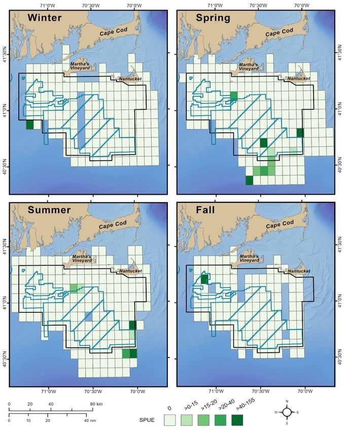
183.1.3.1.1 Relative and absolute abundance
Right whale relative abundance changed throughout the seasons, but they consistently occurred over the
Nantucket Shoals on the eastern side of the survey area (Figure 10). Figure 10 also shows a cluster of
animals using the area south of the MA WEA during the spring.
Figure 10. Sightings per unit effort for right whales during all Campaign 5 aerial surveys
Seasonal numbers of individuals per 1,000 km calculated in 5 x 5 min squares
19Seasonal density and abundance estimates were calculated for right whales for Campaigns 4 and 5 (Table
4); estimates could be calculated for all seasons except summer and fall 2018 (when sightings were either
not on general surveys or did not fall within the truncation distance). Right whale seasonal abundance in
the study area was between two and 92 animals, with the highest abundances occurring consistently in
winter and spring.
Table 4. Density and abundance of right whales during Campaigns 4 and 5 by season and year
Effort (km) is the summed on-effort distance surveyed for all transects. # detections is the number of
sighting of one or more individual animals. # animals is the number of individual animals summed over all
sightings and transects. Est. density is the number of individuals per km2. Est. abundance is the number
of individuals we estimated for the survey area. 95% CI= 95% confidence interval of abundance. * = no
sightings on general surveys, ** = sightings present but they did not occur within the truncation distance.
# of # of Est. Est.
Season-year Effort (km) 95% CI
detections animals Density Abundance
Winter – 17 531 3 7 0.0072 42 7-252
Spring – 17 3606 15 41 0.0062 36 15-85
Summer – 17 1787 1 1 0.0003 2 0-10
Fall – 17 1797 2 2 0.0006 4 1-13
Winter – 18 1579 10 27 0.0093 54 18-167
Spring – 18 1798 3 3 0.0009 5 2-15
Summer – 18 594 * - - - -
Fall – 18 1197 ** - - - -
Winter – 19 2405 30 70 0.0159 92 38-223
Spring – 19 1202 3 23 0.0104 61 6-587
Summer – 19 1202 1 9 0.0041 24 4-135
3.1.3.1.2 Demographic and re-sighting patterns
Photo identification data has not yet been confirmed by the NARWC. This analysis is estimated to be
completed in early 2021. Preliminary photo analysis identified 137 individual right whales during all
Campaign 5 surveys. Most right whales were adults (75%, n = 103) and males (55%, n = 75) (Table 5).
Table 5. Number and percentage of different sex and age classes of right whales identified during
Campaign 5 aerial surveys
Note: * includes one 2019 calf.
Age
Sex N % Adult % Juvenile % %
Unknown
Male 75 55 64 62 11 44 0 0
Female 46 33 34 33 10 40 2 25
Unknown 16 12 5 5 5* 16 6 75
Total 137 100 103 100 26 100 8 100
20You can also read