Methodology to Perform the Reliability Outlook - Published March 2021
←
→
Page content transcription
If your browser does not render page correctly, please read the page content below

2.

Methodology to Perform the
Reliability Outlook
Published March 2021
Caution and Disclaimer
The contents of these materials are for discussion and information purposes and are provided “as is”
without representation or warranty of any kind, including without limitation, accuracy, completeness
or fitness for any particular purpose. The Independent Electricity System Operator (IESO) assumes
no responsibility for the consequences of any errors or omissions. The IESO may revise these
materials at any time in its sole discretion without notice. Although every effort will be made by the
IESO to update these materials to incorporate any such revisions it is up to you to ensure you are
using the most recent version.

Methodology to Perform the Reliability Outlook | March 2021 | Public                                     1

Table of Contents
1.         Introduction                                                 5

2.         Demand Forecasting                                           6
     2.1       Demand Forecasting System                                6
     2.2       Demand Forecast Drivers                                  7
     2.3       Weather Scenarios                                        8

     2.4       Demand Measures                                         11
     2.5       Updating the Demand Forecasting System                  11

3.         Resource Adequacy Risks                                     12
     3.1       Extreme Weather                                         12
     3.2       New Facilities                                          12
     3.3       End of Life of Generation Facilities                    12
     3.4       Generator Planned Outages                               12
     3.5       Lower than Forecast Generator Availability              13
     3.6       Lower than Forecast Hydroelectric Resources             13
     3.7       Wind and Solar Resource Risks                           13

     3.8       Capacity Limitations                                    14
     3.9       Transmission Constrained Resource Utilization           14

4.         Capacity Adequacy Assessment                                16
     4.1       Resource Adequacy Criterion                             16
     4.2       Load and Capacity Model                                 16
     4.3       Data Reported in the Reliability Outlook                17
           4.3.1     Installed Resources/Total Internal Resources      17

           4.3.2     Total Resources                                   18
           4.3.3     Total Reductions in Resources                     18
     4.4       Outputs of the Resource Adequacy Assessment             18

           4.4.1     Required Reserve                                  18
           4.4.2     Reserve Above Requirement                         20

Methodology to Perform the Reliability Outlook | March 2021 | Public    2
4.5 Inputs to the Resource Adequacy Assessment 20
4.5.1 Weekly Available Capacity for Thermal Generating Resources 20
4.5.2 Forecast Hydroelectric Generation Output 21
4.5.3 Capacity Ratings for Wind Generation 23
4.5.4 Capacity Ratings for Solar Generation 24
4.5.5 Available Demand Measures 24
4.5.6 Net Imports 25
4.5.7 Transmission Limitations 25
4.5.8 Forced Outage Rates on Demand of Generating Units Used to Determine the
Probabilistic Reserve Requirement 26
4.5.9 Demand Uncertainty Due to Weather to Determine the Probabilistic Reserve
Requirement 26
5. Additional Considerations in the 42 Month Horizon Error! Bookmark not defined.
6. Energy Adequacy Assessments 28
6.1 EAA Overview 28
6.1.1 EAA Generation Methodology 29
6.1.2 Combustion and Steam Units 29
6.1.3 Nuclear 30
6.1.4 Biofuel 30
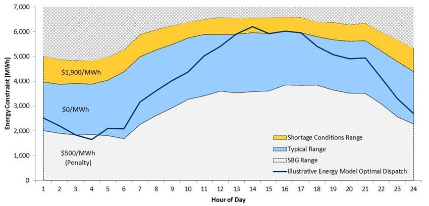
6.1.5 Hydroelectric 31
6.1.6 Wind 32
6.1.7 Solar 33
6.1.8 Demand Measures 33
6.1.9 EAA Demand Forecast Methodology 33
6.1.10 EAA Network Model 33
6.1.11 Forecast of Energy Production Capability 35
7. Transmission Adequacy Assessment 36
7.1 Assessment Methodology for the 18-Month Period 36
7.1.1 Transmission Outage Plan Assessment Methodology 36
7.2 Assessment Methodology for 42 month horizon Error! Bookmark not defined.
Methodology to Perform the Reliability Outlook | March 2021 | Public 38. Operability Assessments 38
8.1 Surplus Baseload Generation (SBG) 38
List of Figures
Figure 2-1 | Creating Monthly Normal Weather – January ................................................ 10
Figure 4-1 | Summary of Inputs and Outputs of L&C ........................................................ 17
Figure 4-2 | Capacity on Outage Probability Table – Graphical Example.......................... 19
Figure 4-3 | Seven-Step Approximation of Normal Distribution – Example ..................... 27
Figure 6-1 | Quadratic Best Fit I-O Equation for a Particular Combustion Generator ...... 29
Figure 6-2 | Nuclear Manoeuvering Unit Dispatch Illustration ......................................... 30
Figure 6-3 | Hydroelectric Solution for a Particular Weekday vs. Hourly and Daily Energy
Constraints ........................................................................................................................... 32
Figure 6-4 | Wind Simulation versus Energy Model Dispatch for a Particular Unit .......... 33
List of Tables
Table 2-1 | Weather Scenarios.............................................................................................. 8
Methodology to Perform the Reliability Outlook | March 2021 | Public 41. Introduction This document describes the methodology used to perform the Ontario Demand forecast, the associated resource and transmission adequacy assessments, and operability assessments for the IESO Reliability Outlook. Over time, the methodology may change to reflect the most appropriate approach to complete the Outlook process Methodology to Perform the Reliability Outlook | March 2021 | Public 5
2. Demand Forecasting
The demand forecasts presented in the Outlook documents are generated to meet two main
requirements: the market rules and regulatory obligations. The Ontario Electricity Market Rules
(Chapter 5 Section 7.1) require that a demand forecast for the next 18 months be produced and
published on a quarterly basis by a set date. The IESO is also required to file both actual and forecast
demand related information with the Ontario Energy Board, the Northeast Power Coordinating
Council and the North American Electricity Reliability Corporation. These regulatory obligations have
specific needs and timelines and the IESO’s forecast production schedule has been designed to
satisfy those requirements.

2.1 Demand Forecasting System
Ontario Demand is the sum of coincident loads plus the losses on the IESO-controlled grid. Ontario
Demand is calculated by taking the sum of injections by registered generators, plus the imports into
Ontario, minus the exports from Ontario. Ontario Demand does not include loads that are supplied by
generation not participating in the market (embedded generation).
The IESO forecasting system uses multivariate econometric equations to estimate the relationships
between electricity demand and a number of drivers. These drivers include weather effects, economic
and demographic data, calendar variables, conservation and embedded generation. Using regression
techniques, the model estimates the relationship between these factors and energy and peak
demand. Calibration routines within the system ensure the integrity of the forecast with respect to
energy and peak demand, and zonal and system wide projections.
We produce a forecast of hourly demand by zone. From this forecast the following information is
available:
•    Hourly peak demand

•    Hourly minimum demand
•    Hourly coincident and non-coincident peak demand by zone
•    Energy demand by zone
These forecasts are generated based on a set of assumptions for the various model drivers. We use a
number of different weather scenarios to forecast demand. The appropriate weather scenarios are
determined by the purpose and underlying assumptions of the analysis. An explanation of the
weather scenarios follows in section 2.3.
Though conservation and demand management are often discussed together, for the purposes of
forecasting, they are handled differently. Demand management is treated as a resource and is based
on market participant information and actual market experience. Conservation projections are
incorporated into the demand forecast. A similar approach is used to quantify the impact of
embedded generation. A further discussion on demand management can be found in section 2.4.

Methodology to Perform the Reliability Outlook | March 2021 | Public                                   6
2.2       Demand Forecast Drivers
Consumption of electricity is modelled using six sets of forecast drivers: calendar variables, weather
effects, economic and demographic conditions, load modifiers (time of use and critical peak pricing),
conservation impacts and embedded generation output. Each of these drivers plays a role in shaping
the results.
Calendar variables include the day of the week and holidays, both of which impact energy
consumption. Electricity consumption is higher during the week than on weekends and there is a
pattern determined by the day of the week. Much like weekends, holidays have lower energy
consumption as fewer businesses and facilities are operating.
Hours of daylight are instrumental in shaping the demand profile through lighting load. This is
particularly important in the winter when sunset coincides with increases in load associated with
cooking load and return to home activities. Hours of daylight are included with calendar variables.

Weather effects include temperature, cloud cover, wind speed and dew point (humidity). Both
energy and peak demand are weather sensitive. The length and severity of a season’s weather
contributes to the level of energy consumed. Weather effects over a longer time frame tend to be
offsetting resulting in a muted impact. Acute weather conditions underpin peak demands.
For the Ontario Demand forecast, weather is not forecast but weather scenarios based on historical
data are used in place of a weather forecast. Load Forecast Uncertainty (LFU) is used as a measure
of the variation in demand due to weather volatility. For resource adequacy assessments a Monthly
Normal weather forecast is used in conjunction with LFU to consider a full range of peak demands
that can occur under various weather conditions with a varying probability of occurrence. This is
discussed further in Section 2.3.
Economic and demographic conditions contribute to growth in both peak and energy demand. An
economic forecast is required to produce the demand forecast. We use a consensus of four major,
publicly available provincial forecasts to generate the economic drivers used in the model.
Additionally, we purchase forecast data from several service providers to enable further analysis and
provide insight. Population projections, labour market drivers and industrial indicators are utilized to
generate the forecast of demand.
Population projections are based on the Ministry of Finance’s Ontario Population Projections.
Conservation acts to reduce the need for electricity at the end-user. The IESO includes demand
reductions due to energy efficiency, fuel switching and conservation behaviour under the category of
conservation. Information on program targets and impacts, both past and future, are incorporated
into the demand forecast.
Embedded generation reduces the need for grid supplied electricity by generating electricity on
the distribution system. Since the majority of embedded generation is solar powered, embedded
generation is divided into two separate components – solar and non-solar. Non-solar embedded
generation includes generation fueled by biogas and natural gas, water and wind. Contract
information is used to estimate both the historical and future output of embedded generation. This
information is incorporated into the demand model.

Methodology to Perform the Reliability Outlook | March 2021 | Public                                     7
Load modifiers account for the impact of prices. The Industrial Conservation Initiative (ICI) and
time of use prices (TOU) put downward pressure on demand during peak demand periods. These
impacts are incorporated into the model.

2.3 Weather Scenarios
Since weather has a tremendous impact on demand, we use a variety of weather scenarios in order
to capture the variability in both demand and weather. The weather scenarios are defined by:
•    The normalization period – daily, weekly, monthly or seasonal
•    The weather selected – mild, normal or extreme

The normalization period refers to the time span over which the weather data is grouped. We use
weekly and monthly normalized weather. The weather selection method determines how you select
the scenario from the data for the normalization period. We select data based on minimum values
(mild scenarios) median values (normal scenarios) or maximum values (extreme scenarios). Based on
these two parameters, we could conceivably have six different weather scenarios Table 2-1 shows
the weather scenarios from the various combinations.

Table 2-1 | Weather Scenarios

Weather Scenarios                   Weekly Normalization Period        Monthly Normalization Period

Mild                                Weekly Mild                        Monthly Mild

Normal                              Weekly Normal                      Monthly Normal

Extreme                             Weekly Extreme                     Monthly Extreme

Here are some key notes on the weather scenarios:
•    We use monthly normalization for the winter and summer seasons as we deem it better captures
     the elements that are needed in our analysis.
•    Monthly normalization results in higher peak demands and lower minimums as compared to daily
     or weekly normalization. This is due to the large set of sorted and grouped data that allows for
     more differentiation between the weather that is most influential and the weather that is least
     influential.
•    The Mild scenarios are used least. Some financial analysis and minimum demand analysis use
     these scenarios.
•    The Normal scenarios are used for reliability analysis for both energy and peak demand.
•    The Extreme weather scenarios are used to study the system in extremis. They are not used for
     energy analysis as sustained Extreme weather is highly unlikely.

Methodology to Perform the Reliability Outlook | March 2021 | Public                                    8
Each of the scenarios has an associated LFU that captures the variability of the weather scenario. For a Mild weather scenario the LFU would be very large as the potential for colder or hotter weather is significant. Conversely, the LFU for an Extreme weather scenario will be quite small as the possibility of exceeding those values is slim. Usually the weather scenario and its LFU are used in a probabilistic approach to generate a distribution of potential outcomes acknowledging the variability of weather and its impact on demand. As stated earlier, the purpose and assumptions underlying each analysis will help determine the appropriate weather scenario to use. In conducting energy analysis it would be inappropriate to use Extreme weather as the likelihood of observing sustained extreme weather is highly unlikely. However, in assessing the system’s capability to meet a one hour summer peak, a Monthly Extreme peak demand forecast would be more appropriate. The weekly resource adequacy assessments in the 18-Month Outlook documents use demand forecasts based on Monthly Normal weather and their associated LFU. Unlike the weather scenarios, which are derived to provide point forecasts under different weather conditions, LFU is used to develop distributions of possible outcomes around those point forecasts. For the summer and winter, Monthly Normal weather is used, and Weekly Normal weather is used for the spring and fall. The Normal weather and the associated LFU are therefore used on a probabilistic basis over the study period. The Extreme weather scenario does not directly translate into probabilistic terms since it is based on severe historic weather conditions. The exact probability associated with the Extreme weather scenario varies by week, month or season. In some instances, the Extreme weather value lies outside of two standard deviations and in other cases it lies within two standard deviations. This is not illogical for any given week as history may have provided an unusual weather episode that will not be surpassed for many years, whereas another week may not have encountered an unusual weather episode. In addition to these weather scenarios, historic weather years are used in certain studies. The years that are typically used are: 1976-77 (typical winter), 1990 (typical summer), 1993-94 (extreme winter), 1995 (extreme summer and winter), 2002 (extreme summer) and 2005 (hot summer). These studies are of particular value when looking at specific events in those years – be it in Ontario or surrounding jurisdictions. An additional weather scenario was created to analyze the hourly allocation of resources. The purpose of this analysis was to evaluate the allocation of resources under sustained high levels of demand. In order to generate this hourly demand profile, a “challenging” weather week was selected from history. The weather was deemed challenging if it led to both a high peak demand and sustained energy demand. A study of the history (1970-2005) led to the selection of a week from January 1982 and a week from August 1973 as challenging winter and summer weather weeks. This weather data was used to generate an hourly demand forecast that was, in turn used to evaluate the resource allocation. To better illustrate the weather scenarios, let’s look at how a scenario is developed. For this example we will look at the Monthly Normal weather for January. Methodology to Perform the Reliability Outlook | March 2021 | Public 9
We use a rolling 31 years of weather data to generate Normal and Extreme weather scenarios. For
each historical day, the daily weather can be converted into a "weather factor" based on wind, cloud,
temperature and humidity conditions for that day. This weather factor represents that days’ weather
in a MW demand impact. Therefore, each day in January from the 31 year history is converted into a
number based on that day's weather. Then, within each month, the 31 days are ranked from highest
to lowest weather impact. Next, the median value of the highest ranked days becomes the highest
ranked day in the Normal month. The median value of the second highest ranked days becomes the
second highest ranked day in the Normal weather. This is repeated until 31 Normal days are
generated for January. This is depicted in Figure 2-1.

Figure 2-1 | Creating Monthly Normal Weather – January

The median number 4,921 corresponds to January 21st, 1976. Therefore, the "coldest" day for
January in the Monthly Normal weather scenario is represented by that day’s weather. Similarly, the
mildest day (1,452) in the Monthly Normal weather scenario for January is represented by January
4th, 2002.
This process is repeated for all the months of the year to finish generating the Monthly Normal
weather scenario. The process is the same for Seasonal and Weekly Normal weather. In order to
generate the Extreme weather scenarios, the maximum value is taken rather than the median in the
above example. Likewise, the Mild scenario is based on minimum values. The LFU is calculated based
on the distribution of weather factors within the weather scenario.
The demand values presented in the Outlook documents are based on Normal weather unless
otherwise specified.
After the representative days are selected for the weather scenarios, they need to be mapped to the
dates to be forecast. They are mapped in a conservative approach ensuring that peak-maximizing-
weather will not land on a weekend or holiday. This allows for consistent inter-week comparison and
a smoother weekly profile. The monthly and seasonal weather scenarios are mapped to the calendar
based on the profile of the weekly scenarios.

Methodology to Perform the Reliability Outlook | March 2021 | Public                                  10
2.4 Demand Measures
The demand measures, which are dispatchable loads and resources secured under the DR Auction,
are treated as resources in the assessment. As such, the reductions due to these programs are added
back to the historical hourly demand. This ensures that the impacts are not counted twice – as a
resource capacity and as lower demand.
These programs are summed to determine a total capacity number. Using historical data we
determine the quantity of reliably available capacity for each zone. Since demand management
programs act like resources that are available to be dispatched, we treat this derived capacity as a
resource in our assessments.

2.5       Updating the Demand Forecasting System
There are several tasks that are carried out on a regular basis as part of the Outlook process:
•    The models are updated for actual data prior to each forecast and the equations are re
     estimated. This enables the system to consistently “learn” from new data.
•    The weather scenarios are updated to include the most recent weather data.

•    A new economic forecast is generated for the economic drivers in the model.
•    Updated conservation data and the performance of demand measures are obtained and
     processed.
The system will therefore include recent experience and the forecast will be based on the most
recent weather scenarios and economic outlooks.

Methodology to Perform the Reliability Outlook | March 2021 | Public                                   11
3. Resource Adequacy Risks The Outlook considers two scenarios, Firm and Planned. The forecast reserve levels for the scenarios should be assessed bearing in mind the risks discussed below. 3.1 Extreme Weather Peak demands in both summer and winter typically occur during periods of extreme weather. Unfortunately, the occurrence and timing of extreme weather is impossible to accurately forecast far in advance. The impact of extreme weather was demonstrated in the first week of August 2006, when Ontario established an all-time record demand of 27,005 MW. Over 3,000 MW of this demand was due to the higher than average heat and humidity. In order to illustrate the impact of extreme weather on forecast reserve levels during the first 18 month, reserves were re calculated assuming extreme weather in each week in place of normal (median) weather. While the probability of this occurring in every week is very small, the probability of an occurrence in any given week is greater (about 2.5 percent). When one looks at the entire summer or winter periods, the expectation of at least one period of extreme weather becomes very likely. The lower reserve levels, under extreme weather illustrates circumstances could arise under which reliance on a combination of non-firm imports, rejection of planned generator maintenance or emergency actions may be required. 3.2 New Facilities The risk of new facilities having a delayed connection to the system is accounted for in the 18 month horizon by considering two resource scenarios: a Firm Scenario and a Planned Scenario. The Firm Scenario considers the existing installed resources, their status change such as retirements and shutdowns over the Outlook period and resources that reached commercial operation. On top of this, the Planned Scenario assumes that all new resources are available as scheduled. The capacity assumed for new resources is the greater of the contracted capacity, or where facilities have begun the market registration process, the capacity submitted to the IESO as part of their registration. 3.3 End of Life of Generation Facilities Generation retirement risks are accounted for in the 18 month horizon in the two resource scenarios. In the Firm Scenario, all resources are removed at end of their contract term. Resources that forecast (via their Form 1230 submission) continued operations are included in the Planned Scenario. 3.4 Generator Planned Outages Methodology to Perform the Reliability Outlook | March 2021 | Public 12
A number of large generating units perform their maintenance in the spring and are scheduled to
return to service from outage prior to summer peak. Meeting these schedules is critical to
maintaining adequate reserve levels. Delays in returning generators to service from maintenance
outages could lead to reliance on imports and/or cancellation of other planned generator outages.
Historically a number of generator outages had to be scheduled during the spring and fall “shoulder
months” due to the dual peaking nature of the Ontario system. The system has transitioned from
dual peaking into summer peaking. This phenomenon together with more new resources creates
some opportunities for generators to schedule their outages in winter months as well. These
opportunities should provide generators with more flexibility to schedule their maintenance outages
which should in turn provide greater assurances going forward that Ontario’s generation fleet will be
well prepared for the high demand summer months.

Information from the 18-Month Outlook report directly feeds into the IESO’s Outage Management
process. Outages are assessed against the firm resource, extreme weather conditions from a
resource adequacy standpoint. Up to 2,000MW of import capability may be relied upon in extreme
weather conditions, and therefore outages on resources (both transmission and generation) that
affect resource availability beyond -2,000MW of Reserve Above Requirement (RAR) are at risk of
being rejected, revoked or recalled. Events that reduce Ontario’s ability to import power such as
outages on interties, internal system constraints, and conditions of neighbouring jurisdictions will be
considered, and the import assumption is adjusted accordingly between zero and two thousand
megawatts.

3.5       Lower than Forecast Generator Availability
IESO resource adequacy assessments include a probabilistic allowance for random generator forced
outages of thermal generators. Along with weather-related demand uncertainty, the impact of
random generator forced outages is included in the determination of required resources.

3.6       Lower than Forecast Hydroelectric Resources
The amount of available hydroelectric generation is greatly influenced both by water-flow conditions
on the respective river systems and by the way in which water is utilized.
It is not possible to accurately forecast precipitation amounts far in advance. Drought conditions over
some or all of the study period would lower the amount of generation available from hydroelectric
resources. Low water conditions can result in significant challenges to maintaining reliability, as was
experienced in the summer of 2012. As such, in the extreme weather scenario of the 18-Month
Outlook, the hydroelectric conditions are based on the median production at peak in the summer of
2012.

3.7       Wind and Solar Resource Risks
The Outlook assumes monthly Wind Capacity Contribution Solar Capacity Contribution values to
forecast the capacity contribution from wind and solar generators, respectively. There is a risk that
wind power output could be less than the forecast values.

Methodology to Perform the Reliability Outlook | March 2021 | Public                                      13
3.8       Capacity Limitations
There is a risk that any given generator may not be capable of producing the maximum capacity that
the market participant has forecast to be available at the time of peak demand. There may be several
reasons for these differences. Independent of the best efforts of generator owners to maintain
generator capability, there are sometimes external factors which may impact the capability to
produce.
Some outages and deratings, such as environmental limitations and high ambient temperature
deratings, may be more likely to occur at roughly the same time as the extreme weather conditions
that drive peaks in demand.
For example, there are risks that gas-fired generators may not be capable of producing the maximum
capacity that the market participant has forecast to be available at the time of peak. The natural gas
and electricity sectors are converging as natural gas becomes one of the more common fuels in North
America for electric power generation. The IESO is jointly working with the Ontario gas transportation
industry to identify and address issues.

3.9       Transmission Constrained Resource Utilization
Transmission constraints may occur more often than expected due to multiple unplanned outages
and may also have greater impact than expected on the ability to deliver generation to load centres.
This is particularly true for large transformers whose repair or replacement time can be much longer
than for transmission lines. Although many transmission limitations are modelled in accordance with
recognized reliability standards, limitations resulting from multiple forced transmission outages can
have significant impacts on resource availability.
Constraints may also occur due to weather conditions that result in both high demands and higher
than normal equipment limitations. For example periods of low wind combined with hot weather not
only cause higher demands but also result in lower transmission capability. This can affect the
utilization of internal generation and imports from neighbouring systems at critical times.
Transmission constraints that result from loop flows can be particularly hard to predict because they
result not only from the conditions within Ontario but from the dynamic patterns that are taking place
within and between other areas. Depending on the direction of prevailing loop flows, this may
improve or aggravate the ability to maintain reliability.
During high demand periods, the availability of high-voltage capacitors and the capability of
generators to deliver their full reactive capability also become critically important for controlling
voltage to permit the higher power transfers that are required. Outages or de-ratings to these
reactive resources can restrict power transfer from generators and imports, and make it difficult to
satisfy the peak demands.
The calculated values at the time of weekly peak for transmission constrained generation presented
in the IESO Reliability Outlook Tables correspond to a generation dispatch that would maximize the
possible reserve above requirements in Ontario. However, in real time operation, the actual amount
of bottled generation will depend on many conditions prevailing at the time, including the local
generation levels, overall generation dispatch and the direction and levels of flows into and out of
Ontario. Electricity supply from some baseload generation sources may have to be decreased during
times when transmission constraints and tight supply conditions prevail.

Methodology to Perform the Reliability Outlook | March 2021 | Public                                    14
Methodology to Perform the Reliability Outlook | March 2021 | Public 15
4. Capacity Adequacy Assessment
This section describes the criterion, tools and methodology the IESO uses to perform resource
adequacy assessments. In Section 4.1, the resource adequacy criterion is described. Section 4.2
describes the Load and Capacity (L&C) software tool used in the resource adequacy assessment
process. Section 4.5 presents the inputs used in the capacity adequacy assessment.

4.1       Resource Adequacy Criterion
The IESO uses the NPCC resource adequacy design criterion as provided in the NPCC “Directory #1:
Design and Operation of the Bulk Power System” to assess the adequacy of resources in the Ontario
Area. The NPCC resource adequacy criterion (Requirement 4 in Directory #1) states:

    R4: Each Planning Coordinator or Resource Planner shall probabilistically evaluate resource
    adequacy of its Planning Coordinator Area portion of the bulk power system to demonstrate that
    the loss of load expectation (LOLE) of disconnecting firm load due to resource deficiencies is, on
    average, no more than 0.1 days per year.
    R4.1 Make due allowances for demand uncertainty, scheduled outages and deratings, forced
    outages and deratings, assistance over interconnections with neighboring Planning Coordinator
    Areas, transmission transfer capabilities, and capacity and/or load relief from available operating
    procedures.

4.2       Load and Capacity Model
The IESO uses the Load and Capacity (L&C) model to evaluate the resource adequacy for each week
in the study period consistent with the NPCC resource adequacy criterion.
Figure 4-1 describes, visually, the interaction between the inputs into and outputs from L&C. The
Total Resources, shown in the far left, are values used for reporting purposes and are not part of the
analysis. This indicates the total resources in Ontario, without prejudice to their availability or
capability to serve Ontario’s load. The Available Resources, shown in the centre, are the inputs
relating to generation or demand measures that can be expected to serve Ontario’s load. The
assumptions used to develop these inputs are described in Section 4.5. At a high level, the key inputs
to determine Available Resources are:
•    Thermal generating units’ net maximum continuous rating (MCR),
•    Thermal generating units’ planned outages and deratings,
•    Forecast hydroelectric generation output
•    Wind capacity contribution (WCC) values
•    Solar capacity contribution (SCC) values for, and

Methodology to Perform the Reliability Outlook | March 2021 | Public                                      16
• The forecast demand, whose methodology was described in Section 2.
The output of the L&C model is the required reserve (described in Section 4.4) to ensure that the
resource adequacy criterion is met. The inputs that are used to determine the probabilistic required
reserve are:
• Demand forecast and its uncertainty and
• Thermal generating units’ forced outage rates on demand.
Figure 4-1 | Summary of Inputs and Outputs of L&C
4.3 Data Reported in the Reliability Outlook
The following section describes data that is reported in the Reliability Outlook but is not used in the
L&C tool to determine required reserve.
4.3.1 Installed Resources/Total Internal Resources
The Installed Resources (also called Total Internal Resources) is not used in the L&C tool, but rather
is a value used to report the total installed capacity of resources connected to and participating in the
IESO Administered Energy Market. It is made up of two components; the first is the existing supply
(generation) resources, which are presented in Table 4.1. For the existing supply, only resources that
have completed the final milestone in the Market Registration timeline are included as existing
resources. The capacities of these resources (referred to here as Installed Capacity of each resource)
are determined by referring to two sources of data:
• Data provided by Market Participants via Online IESO, as part of the Market Registration process:
the Maximum Active Power Capability (the maximum active power capability under any conditions
without station service being supplied by the unit. This value will be used to calculate the energy
resource’s maximum offer capability), is retrieved from the IESO’s Customer Data Management
System for all facilities that have completed Market Registration.
Methodology to Perform the Reliability Outlook | March 2021 | Public 17• For some resources, there may be additional restrictions on their maximum capability, as
determined during commissioning. In these cases, the IESO may further reduce their Installed
Capacity using information provided in their Commissioning report.
To estimate future Installed Resources on a weekly basis (as shown in Table A1 of the IESO
Reliability Outlook), expected changes shown in Table 4-1 as Firm Capacity are added or subtracted
from the existing supply.
4.3.2 Total Resources
The Total Resources are the summation of the Installed Resources and the Firm Net Imports.
4.3.3 Total Reductions in Resources
Where any tables in the IESO Reliability Outlook reference Reductions to Total Resources, these
reductions are relative to the Total Resources described above. Reductions are made up of
differences between the Total Resources and the:
• Available Capacity of Thermal Resources;
• Forecast Hydroelectric Generation Output;
• Capacity Ratings for Wind Resources;
• Capacity Ratings for Solar Resources;
• Available Demand Measures; and
• Transmission Limitations.
4.4 Outputs of the Resource Adequacy Assessment
4.4.1 Required Reserve
Reserves are required to ensure that the forecast Ontario Demand can be supplied with a sufficiently
high level of reliability. The Required Resources is the amount of resources needed to supply the
Ontario Demand and meet the Required Reserve as shown in Figure 4-1. The Reserve Above
Requirement is the difference between Available Resources and Required Resources.
The Required Reserve is a planning parameter that, depending on the type of assessment, takes into
account the uncertainty associated with demand forecasts or generator forced outages in a
probabilistic or deterministic approach. The output of L&C is the amount of Required Reserve, in MW
and as a percentage of forecast demand, for each week in the study period.
The amount of Required Reserve to meet the resource adequacy criterion is calculated on a week-by-
week basis as the maximum of a deterministically and a probabilistically calculated reserve
requirement. These two reserve requirements are described in this section.
Methodology to Perform the Reliability Outlook | March 2021 | Public 18Probabilistic Reserve Requirement A resource adequacy criterion equivalent to an LOLE of 0.1 days per year is used to determine the probabilistic reserve requirement for each week of the planning year. The program uses the ‘direct convolution’ method to calculate the weekly probabilistic reserve requirement. The probabilistic reserve requirement consider two inputs in a probabilistic manner: demand uncertainty and forced outages and deratings of thermal units. The inputs for these are described in Section 4.4 . The available capacity and forced outage rates on demand of thermal generation units are used to build a Capacity on Outage Probability Table (COPT) which contains the cumulative probabilities of having various amounts of generating capacity or more on forced outage. A graphical example is shown in Figure 4-2. Figure 4-2 | Capacity on Outage Probability Table – Graphical Example In the L&C model, a normal distribution of demand values around the mean demand value is assumed, as described in Section 4.1.5. The probabilistic reserve requirement calculation is executed in an iterative manner. In each iteration, an amount of Generation Reserve is assumed and an associated LOLE is calculated by convolving the LFU corresponding to the peak demand value with the COPT. The iterative process is repeated with small changes to the assumed Generation Reserve until the calculated LOLE becomes equal to or less than the target. When this condition becomes true, the assumed level of Generation Reserve equals the probabilistic required reserve necessary to meet the reliability target. Methodology to Perform the Reliability Outlook | March 2021 | Public 19
Deterministic Reserve Requirement
The deterministic reserve requirement for each week is equal to the Operating Reserve (equal to the
first single largest contingency plus half the size of the next largest contingency), plus half the size of
the second largest contingency plus the absolute value of the LFU.

4.4.2 Reserve Above Requirement
The adequacy of the Available Resources to meet the demand over the study period can then be
assessed in an arithmetic calculation illustrated in Figure 4-1. The Reserve Above Requirement is
obtained by subtracting the Required Resources (equal to the peak demand plus Required Reserve)
from the Available Resources.
It should be noted that negative Reserve Above Requirement values in some weeks do not
necessarily mean a violation of the NPCC resource adequacy criterion. This may only mean higher
risk levels for the respective weeks. Whenever negative Reserve Above Requirement values are
identified, the possible control actions to restore the reserves to required levels are considered and
assessed.

4.5       Inputs to the Resource Adequacy Assessment
For each planning week, the expected level of Available Resources is determined, considering:
•    The amount of generator deratings;

•    Planned and long term unplanned generator outages;
•    Generation constrained off due to transmission interface limitations;
•    Any capacity imports or exports backed by firm contracts;

•    Any imports identified by market participants to support planned outage requests to the IESO;
     and
•    The assumed amount of price responsive demand.
The expected level of Available Resources is calculated using the outage profile associated with the
maximum outage day in each planning week, i. e. the day with the maximum amount of unavailable
generating capacity in that week. Although the weekly peak does not always occur on the maximum
outage day, such coincidence is assumed for the determination of Available Resources.

4.5.1 Weekly Available Capacity for Thermal Generating Resources
The maximum capability for most thermal generating resources, such as nuclear, biofuel and gas
fired generators, is affected by external factors, such as ambient temperature and humidity or
cooling water temperature. To capture those variables, the Maximum Continuous Rating (or “MCR”)
for each thermal generator is modelled on a monthly basis.
Nuclear generators and the like whose MCR is not ambient temperature sensitive provide monthly
gross MCR and their station service load in their annual Form 1230 submission and this MCR is
entered as a direct input in the L&C tool.

Methodology to Perform the Reliability Outlook | March 2021 | Public                                     20
Fossil- or biofuel-fired generators whose MCR is sensitive to ambient temperature provide, through their annual Form 1230 submission, gross MCR at five different temperatures specified by the IESO which are used to construct a temperature derating curve. For each such generator, two monthly gross MCR values - one for the normal weather scenario and the second for the extreme weather scenario - are calculated at representative monthly temperatures using the derating curve. Each zone’s two monthly representative temperatures are determined from historical data collected from the weather station assigned to that zone based on proximity. For normal weather scenario, the zonal representative temperature is the median of the daily peak temperatures in the month in the zone. The zonal representative temperature for the extreme weather scenario is the maximum of the daily peak temperatures in the month in that zone for the months from April to October. For the months from November to March, the temperature for the extreme weather scenario is the minimum daily temperature in the month in each zone; the cold temperature is capped at -10°C. Generators also provide their station service load annually which is allocated in proportion to the size of each unit at the station to calculate net MCR values for each unit. The IESO updates the net MCR values annually in the second quarter using the data generators submit on Form 1230 by April 1. If an existing generator is expected to shut down during the study timeframe, then the MCR is set to 0 MW beginning the week it is expected to expire. For example, for NUG whose contract expires during the Outlook period, its installed capacity and its rating are both set to zero beginning in the week of its contract expiry in the firm scenario. Planned outages and deratings, as well as any forced outages that extend into the horizon of the 18 Month Outlook, are extracted from the IESO’s outage management system. An outage profile for all thermal generators is calculated as an input into L&C using two steps: 1. Determine the maximum outage day (MOD) in each planning week. This is the day with the maximum amount of unavailable generating capacity in that week. 2. For the MOD selected, sum up the outages that occur during the daily peak window (currently hour ending 15 to 22). This is the window where the weekly peak demand is expected to occur. This ensures that outages covering the overnight off-peak hours do not affect the generation unavailability total of the MOD and consequently do not affect the Reserve Above Requirement. Although the weekly peak does not always occur on the maximum outage day, such coincidence is assumed for the determination of Available Resources. 4.5.2 Forecast Hydroelectric Generation Output The forecast hydroelectric generation output is calculated using median historical values of hydroelectric production and contribution to operating reserve during weekday peak demand hours to create a dataset of historic production. The details for developing the generation output forecast are described in this subsection. Methodology to Perform the Reliability Outlook | March 2021 | Public 21
First, data of historical hydro production at the time of every non-holiday weekday are collected. For
every non-holiday weekday since market open, the IESO selects the one individual hour that the daily
peak demand occurred. The selection of the weekday peak demand hour may differ from day-to-day
in the same month and can vary for the same month in different years as the demand profile
changes from year-to-year. Once the daily peak is selected, the following pieces of data coincident to
the peak are extracted:
•    Hydro production (Allocated Quantity of Energy Injected or AQEI)

•    Scheduled operating reserve in the constrained schedule
•    Installed capacity
•    Effects of historical outages on capability across the fleet

Since a large number of Ontario’s hydroelectric generators are not run of river, this method assumes
that regardless of what hour the peak may occur, the hydroelectric fleet would be scheduled in a
manner that allows its output to peak coincident to when the Ontario demand peaks.
This new data set is then used to determine, on a monthly basis, the hydroelectric generation output
forecast, which is shown in Table 4.3 of the Reliability Outlook. The “Historical Hydroelectric Median
Contribution” is determined by:
1. For each hour in the data set, summing the hydro production and scheduled OR together
   (“generation output”)

2. Grouping the generation output by month
3. Normalizing the generation output by the installed capacity of hydro generation. This
   normalization converts the generation output into a ratio of generation output to installed
   capacity.
4. Calculating the median for each month.
5. Multiplying each monthly capacity factor by the current hydroelectric Installed Capacity (all units
   currently in-service).
This calculation includes the impacts of hydroelectric outages. The expected capability of individual
hydroelectric resources that were on planned outage and not injecting into the IESO grid is then
estimated and added back into the historic production data. This allows the IESO to estimate the
capability of the hydroelectric fleet if there were no outages. The following steps are used to “add
back” the impacts of outages from the historic data. The end result of this calculation is presented in
the Reliability Outlook as “Historical Hydroelectric Median Contribution without Outages.”
1. For each hour since market open, the IESO retrieves the hydro capacity that was on a planned
   outage. This creates an hourly profile of the capacity unavailable due to outages, but it
   overestimates the impact, as not all of a generator would have been available as fuel limitations
   impact hydro output. Because of this, the hourly unavailable capacity as a result of planned
   outage is multiplied by a capacity factor that changes by month and zone. This capacity factor is
   calculated from historical norms. This creates an effective loss of capability due planned outages.
2. The amount of effective hydroelectric capability loss during the historical daily peak hour is added
   back to the historical contribution. This final value is the hydroelectric capability estimate

Methodology to Perform the Reliability Outlook | March 2021 | Public                                     22
assuming all units in-service. This is done so that we may discount hydroelectric capability by the
     effects of future planned outages over the planning timeframe. This step is necessary to ensure
     we are able to assess hydroelectric outages and its impact on resource adequacy.
The Forecast Hydroelectric Generation Output, which is ultimately input into L&C, takes into account
the impacts of planned outages and deratings on a weekly basis. The IESO performs the following
steps to create this estimate:

1. Planned outages and deratings that extend into the horizon of the outlook are extracted from the
   outage management system. The outages considered are only those that occur on the Maximum
   Outage Day of the week within the daily peak period.
2. The total reduction in the outage management system for each hydroelectric outage/derate is
   multiplied by a zonal capacity factor for the full duration of the outage. This capacity factor, which
   varies by month and zone, is derived from historical analysis of hydro. This is deemed the loss of
   capacity due to outages,
3. The loss of capacity from each outage/derate is summed up to determine the total loss of
   capacity for each week.

4. The weekly loss of capacity is subtracted for each week from the Historical Hydroelectric Median
   Contribution without Outages. This new value is the Forecast Hydroelectric Generation Output.
A review of historical hydroelectric production data during extreme summer period showed that
forecasts based on median values for all years in the sample overstates the availability of
hydroelectric production during the summer extremes. To more accurately reflect hydroelectric
production in the extreme weather scenario, the median contribution of the hydroelectric fleet at the
time of peak for summer months (June to September) is based on 2012 – the driest year in the
sample. This is estimated to be about 800 MW lower than the values for normal weather conditions.
As additional years of market experience are acquired, the driest year will be determined to calculate
the impact. The methodology to calculate the hydroelectric contribution at varying conditions is
continuing to evolve to reflect the actual experience.

4.5.3 Capacity Ratings for Wind Generation
Monthly Wind Capacity Contribution (WCC) values are used to forecast the contribution from wind
generators as a percentage of installed capacity. To calculate the WCC the IESO performs the
following steps:
•    Actual historic median wind generation contribution over the last ten years is compiled. If a wind
     facility was curtailed, the impacts of this foregone energy are added back to the production
     numbers, to estimate what the wind generator was capable of producing at the time. The
     foregone energy is estimated from the 5 minute ahead wind forecast for that wind facility.
•    The top 5 contiguous demand hours are determined by the frequency of demand peak
     occurrences over the last 12 months. The demand hours are calculated for the winter and
     summer season, or shoulder period month.
•    The dataset in step one is filtered for just the top 5 contiguous demand hours.

Methodology to Perform the Reliability Outlook | March 2021 | Public                                   23
• The wind contribution across Ontario coincident to the demand hours previously estimated is
summed together.
• The wind contribution each hour is normalized against the installed capacity of wind at the time
of production.
• The median is then selected for each winter and summer season, or shoulder period month. For
example, the wind generation contribution for summer is made the median generation
contribution in the demand hours for June, July and August combined.
• For each week in the Reliability Outlook, the WCC is multiplied against the expected wind
installed resources (this includes both existing and future wind generators).
4.5.4 Capacity Ratings for Solar Generation
Monthly Solar Capacity Contribution (SCC) values are used to forecast the contribution from solar
generators as a percentage of installed capacity. SCC values in percentage of installed capacity are
determined by calculating the median contribution during the top 5 contiguous demand hours of the
day for each winter and summer season, or shoulder period month. A dataset comprising ten years
of simulated solar production history is used for this purpose. As for wind, the top 5 contiguous
demand hours are determined by the frequency of demand peak occurrences over the last 12
months. As actual solar production data becomes available in future, the process of combining
historical solar data and the simulated 10-year historical solar data will be incorporated into the SCC
methodology, until sufficient actual solar production history has been accumulated, at which point
the use of simulated data will be discontinued.
The SCC is calculated by performing the following steps:
1. The top 5 contiguous demand hours are determined by the frequency of demand peak
occurrences over the last 12 months. The demand hours are calculated for the winter and
summer season, or shoulder period month. These hours are the same as those used for the
WCC.
2. The IESO uses a dataset comprising ten years of simulated solar production history. This dataset
is filtered for just the top 5 contiguous demand hours.
3. The dataset is further filtered to include only the data that represent solar output at a simulated
site closest to where solar generation farms are actually installed in Ontario.
4. The solar contribution across Ontario coincident to the demand hours previously estimated is
summed together. The summation is normalized against the installed capacity of solar.
5. The median is then selected for each winter and summer season, or shoulder period month.
6. For each week in the Reliability Outlook, the SCC is multiplied against the expected solar installed
resources (this includes both existing and future wind generators).
4.5.5 Available Demand Measures
Methodology to Perform the Reliability Outlook | March 2021 | Public 24It is important to distinguish between demand measures and load modifiers. Demand measures include dispatchable loads and capacity secured through the Demand Response Auction. Demand measures are treated as a resource. Load modifiers include embedded generation output, Time of Use Rates and the Industrial Conservation Initiative (ICI). These are incorporated into the demand forecast. The available capacity of dispatchable loads is based on historical offers into the market. For most weeks, the average bid at weekday peak in the last twelve months is used as the available capacity. For weeks that are likely the annual peak, the IESO determines the available capacity from the offers during the top 5 demand hours of the past year. This ensures that the impacts of the ICI program are not double counted, as many dispatchable loads also participate in ICI. The capacity secured through the DR auction is discounted to 69% in the summer and 78% in the winter of what was procured for the obligation period in each season to account for the fact that participants may not always be available. This is based on the weighted average performance of the last five DR test/activation results for each season. 4.5.6 Net Imports The purpose of the IESO Reliability Outlook is to determine a required reserve for Ontario to be self- sufficient. Therefore, the only imports or exports considered are those backed by firm contracts/commitments. Where a contract/commitment exists, the capacity associated with it is calculated for each week of its stated deliverability period. The Net Imports are the Firm Imports less any Firm Exports. For example, if there are no Firm Imports in a given week but there is a Firm Export, then the Net Imports will be a negative number. 4.5.7 Transmission Limitations The available capacity of thermal, hydroelectric, wind and solar resources may be subject to further reductions due to limitations of the transmission system. The IESO-controlled grid consists of a robust southern grid and a sparse northern grid. The northern grid has limitations, which potentially constrain the use of some generation capacity. As well, southern zones of the system could have some generation constrained at times, especially during outage conditions, because of the transmission interface limitations. The amount of generation constrained varies with the demand level, the amount of total generating capacity in a zone as well as the interface transfer capability. All transmission constrained generation is subtracted from the Available Resources. This becomes the final value used in calculating the Reserve Above Requirement. Methodology to Perform the Reliability Outlook | March 2021 | Public 25
4.5.8 Forced Outage Rates on Demand of Generating Units Used to Determine the
Probabilistic Reserve Requirement
Equivalent forced outage rates on demand (EFORd) are used for each thermal generation unit as a
measure of the probability that the unit will not be available due to forced outages and forced
deratings when there is a demand for the unit to generate. The values are calculated by the IESO
using a rolling five years of generator outage and operations data, consistent with IEEE Std 7621.
EFOR data supplied by market participants will continue to be used for comparison purposes. EFORd
impacts Required Reserve and does not impact the Total Reductions in Resources.

4.5.9 Demand Uncertainty Due to Weather to Determine the Probabilistic Reserve
Requirement
The L&C program requires weekly peak demands for the study period. These peak demand values
include loads that may be dispatched off during high price periods, loads that may simply reduce in
response to high prices, and loads that may otherwise be reduced in the case of a shortfall in
reserves. For modelling purposes, the total demand is assumed to be supplied, and is included in the
peak demand forecast when the probabilistic reserve requirement is calculated. To meet the
Required Reserve, the assessment allows that some of the reserve may be comprised of a quantity of
demand that can decrease in response to market signals. The IESO forecasts the future price
responsive demand levels based on Market Participant registered data and consideration of actual
market experience.
The LFU for each week, due mostly to weather swings, is represented by the associated standard
deviation, assuming a normal probability distribution. This data is obtained from weather statistics
going back to 1984, and is updated annually. The weather related standard deviations vary between
about 2% and 7% of their associated mean demand values through the year. Each week’s peak
demand is modelled by a multi-step approximation of a normal distribution whose mean is equal to
the forecast weekly peak and whose standard deviation is equal to the LFU. Subsequently, in the
probabilistic reserve requirement calculation for each planning week, not only the mean value of the
peak demand is included, but also a range of peak demand values, ranging from mild to extreme
demand values. Figure 4.3 illustrates a seven step example of such an approximation, using a weekly
peak value of 23,000 MW and an associated LFU value of 1,000 MW. In this example, the peak
values considered in the probabilistic reserve requirement calculation would range from 20,000 MW
to as high as 26,000 MW. Consequently, the calculated probabilistic reserve requirement reflects not
only the impact of the generation mix (generator sizes and failure rates) but also the impact of
uncertainties in demand related to weather. This is achieved by weighting the impact of each of the
seven peak demand values by its associated probability of occurrence (shown in Figure 4-3 under the
curve).

1 IEEE Standard Definitions for Use in Reporting Electric Generating Unit Reliability, Availability, and Productivity, IEEE Std 762-2006

Methodology to Perform the Reliability Outlook | March 2021 | Public                                                                       26
You can also read