Modelling epidemic spread in cities using public transportation as a proxy for generalized mobility trends - Nature
←
→
Page content transcription
If your browser does not render page correctly, please read the page content below
www.nature.com/scientificreports
OPEN Modelling epidemic spread in cities
using public transportation
as a proxy for generalized mobility
trends
Omar Malik1,2*, Bowen Gong2, Alaa Moussawi3, Gyorgy Korniss1,2 &
Boleslaw K. Szymanski2,4
We study how public transportation data can inform the modeling of the spread of infectious diseases
based on SIR dynamics. We present a model where public transportation data is used as an indicator
of broader mobility patterns within a city, including the use of private transportation, walking etc. The
mobility parameter derived from this data is used to model the infection rate. As a test case, we study
the impact of the usage of the New York City subway on the spread of COVID-19 within the city during
2020. We show that utilizing subway transport data as an indicator of the general mobility trends
within the city, and therefore as an indicator of the effective infection rate, improves the quality of
forecasting COVID-19 spread in New York City. Our model predicts the two peaks in the spread of
COVID-19 cases in NYC in 2020, unlike a standard SIR model that misses the second peak entirely.
Long-range mobility, such as traveling between cities, can cause a disease to spread through case importation
across large distances1, 2. Short-range mobility, such as usage of city buses or trams, has been correlated with
a higher risk of contracting acute respiratory infections3 and with the number of cases of COVID-19 within
cities4, 5. Accordingly, restrictions on human mobility, either directly by shutting down public t ransportation6, 7
or indirectly by restricting public and private g atherings8, which were highly effective in stopping the spread of
COVID-19. We hypothesize that alongside being a high-risk medium for infections, public transportation usage
is also a good indicator for the level of short-range mobility for the entire population of a city.
COVID‑19 in New York City. When it became clear that the COVID-19 virus is highly infectious, New
York City (NYC) imposed restrictions that included shutting-down non-essential businesses and forbidding
large gatherings, but kept public t ransportation9 and schools o
pen10. The usage of NYC’s sprawling subway sys-
tem was found to be correlated with the spread of COVID-194, 5, 11 and mobility patterns in general were cor-
related with the spread of COVID-19 within regions of the c ity12, 13. There are various models of disease spread
that incorporate human mobility patterns, such as a recent disease transmission model inspired by collision
theory gas-phase chemistry14, or a metapopulation model that allows for the movement of individuals between
subpopulations15. We propose a model based on SIR dynamics where we explicitly model human mobility as a
parameter and treat the infection rate as a function of the mobility of a region. To effectively model the spread
of COVID-19 in NYC, we focus on data from the NYC subway. We hypothesize that trends in subway usage are
correlated with the usage of other modes of transport, such as buses, taxis etc. We therefore treat subway usage
as an indicator for broader human mobility patterns in the city.
Data
New York City subway turnstile data. Unlike pedestrian traffic, private automobiles, and to some extent
taxis, public transportation, and in particular the subway, has detailed records of passenger traffic such as the
total number of entries and exits from a station collected in real time. This enables us to extract some important
statistics regarding passenger traffic using publicly available data on subway usage published by the Metropolitan
Transportation Authority (MTA)16. As awareness of the pandemic grew in early 2020 the Governor of New York
1
Department of Physics, Applied Physics, and Astronomy, Rensselaer Polytechnic Institute, Troy, NY 12180,
USA. 2Network Science and Technology Center, Rensselaer Polytechnic Institute, Troy, NY 12180, USA. 3New York
City Council, City Hall Park, New York, NY 10007, USA. 4Department of Computer Science, Rensselaer Polytechnic
Institute, Troy, NY 12180, USA. *email: maliko@rpi.edu
Scientific Reports | (2022) 12:6372 | https://doi.org/10.1038/s41598-022-10234-8 1
Vol.:(0123456789)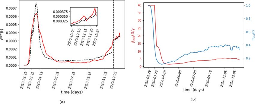
www.nature.com/scientificreports/
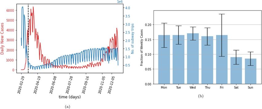
Figure 1. (a) The red line shows the daily reported cases of COVID-19 in New York City. The blue line shows
the total daily number of trips taken on the subway, with entries related to the Port Authority Trans-Hudson
(PATH) removed. The dotted line indicates the start of the NY PAUSE Program, (b) The fraction of total weekly
cases reported on each day of the week, averaged over 44 weeks. While the weekdays remain largely consistent,
there is a significant drop in reporting on weekends.
announced a state of emergency on March 7 2020, followed shortly by the passage of an executive order, known
as ’New York State on PAUSE’, that shutdown all non-essential businesses in the s tate9, 17. New York City saw a
decline in subway usage alongside various other modes of public transport, including b ikeshares18, 19, and t axis20.
As restrictions were slowly eased in the later half of the year, there was a corresponding increase in the usage of
public transport, although some modes were preferred over others at different rates than before the pandemic.
Bikehares, for example, had recovered to their 2019 levels by September 30, 2020 while subway ridership was
at 30% of pre-pandemic levels18. Despite the different rates at which different modes recovered, both bikeshares
and the subway saw increases in usage in the latter half of 2020. We believe that this increase in both modes of
transport corresponds to the underlying increase in human mobility as restrictions were loosened after June 8,
2020. This motivates us to use this directly measurable traffic as a proxy for all traffic in the city.
We collected and analyzed the subway turnstile data of New York City for 12 consecutive months, starting
from January 2020 to December 2020. The MTA publishes turnstile data on a weekly basis, which includes
administrative information such as the control area, unit number, station name and line name, as well as the
counts of the entries and exits at a specific time for a particular t urnstile16. The system collects these counts every
four hours, each of which is a cumulative register value. The data were first converted into dataframes and then
into a combination of control area code, remote unit, subunit channel position (SCP), as well as the time of the
observation that serves as a unique ID to identify and remove duplicate records. We removed entries related to
Port Authority Trans-Hudson (PATH) trains, since they do not represent the mobility among NYC boroughs.
The absolute difference between the first and last counts at a turnstile on a particular day defines the number of
subway riders passing through that particular turnstile. The geographic coordinates of the station and the borders
of each borough allow us to place each station in its corresponding borough. We calculated the total number of
borough-level subway riders by summing the numbers of riders at all the turnstiles of all subway stations located
within each borough. To estimate the mobility between boroughs, we used a survey that was conducted among
subway riders regarding the origin and destination of their trips21. Given the number of departures at a given
station, we used probabilities extracted from the survey to determine the destinations of those trips.
COVID‑19 data. We used publicly available data published by the NYC government about the number of
new COVID-19 cases reported for each day and for each of the five b oroughs22. Figure 1a shows that this data
has a clear weekly cyclical pattern. Figure 1b shows that this pattern arises because of the much smaller numbers
of cases that were reported on weekends than on weekdays. We remove this pattern by using a running 7-day
average of the number of daily cases.
We also chose to restrict our analysis to 2020, since the introduction of vaccines in early 2021 decreases the
number of people susceptible to infection. To account for this decrease on the spread of epidemics would require
the introduction of another parameter that might change the quantitative effect of mobility on the spread of
the disease.
Population data. All population data for New York City were taken from the 2020 census conducted by the
US Census Bureau and published on their website23.
Scientific Reports | (2022) 12:6372 | https://doi.org/10.1038/s41598-022-10234-8 2
Vol:.(1234567890)
www.nature.com/scientificreports/
Model
We start with the well-established SIR model24, 25. While more powerful models for modelling disease spread
exist, such as the SEIR model26, we picked the SIR model in order to reduce the number of parameters and avoid
overfitting. The COVID-19 hospitalization data that we use only reports daily newly infected cases and we do not
believe this data is fine-grained enough to justify the use of a more complex model. The SIR model divides the
total population (N) into susceptible (S), infected (I), and recovered or dead (R) compartments. The equations
governing the spread of the disease are
d S(t)I(t)
S(t) = −β , (1)
dt N
d S(t)I(t)
I(t) = β − γ I(t), (2)
dt N
d
R(t) = γ I(t), (3)
dt
where β and γ are the infection and recovery rate, respectively.
We modify the model by dividing the total population into subpopulations called regions, each with a frac-
tion of the population pj living in region j, thus j pj = 1. When we apply the model to New York City the
different pj represent the populations of the five boroughs of New York City, normalized by the total population
of the city, which was 8,804,190 in 2 02023. Within a region, people will have different infection rates based on
their activity. The infection rate for individuals working from home and following strict quarantine protocols
will be lower than the rate for frontline workers. Each activity-based cohort has an associated infection rate βjc .
Additionally, people may also have access to different quality of healthcare, which may impact the frequency of
testing and the likelihood of visiting a doctor. Both of these parameters influence the recovery rate of a patient.
Each healthcare-based cohort has an associated recovery rate γje . The fraction of the total population in region
j with behavior c and healthcare e is denoted as pjce . For parameters representing the
population fractions, an
omitted index indicates a sum over all values of this index, so pjc = e pjce and pj = c,e pjce etc.
Each cohort within each region follows SIR dynamics. The equations governing the population fractions of
susceptible, infected and recovered individuals are given by:
(4)
sjce (t + �t) = sjce (t) 1 − βjc ijce (t)�t ,
(5)
ijce (t + �t) = ijce (t) + βjc sjce (t)ijce (t) − ijce (t)γje �t,
rjce (t + �t) = rjce (t) + ijce (t)γje �t, (6)
where sjce (t), ijce (t) and rjce (t) are the population fractions of susceptible, infected and recovered individuals,
respectively at time t.
Inter‑region mixing. So far our model follows straightforward SIR dynamics. We now want to introduce
inter-region mixing through a mixing parameter that tells us the population fraction of one region that is visit-
ing another region at a given time. In order to calculate this quantity, we need to know the origin, destination,
and trip duration for every rider using the subway. From the data, we only know the borough of departure. We
do not know an individual rider’s destination based just on the borough they departed from. Using an MTA
survey on the use of the NYC subway, we can determine the probabilities of a trip departing and terminating at
different boroughs21.
In order to determine the average time spent visiting a borough, we also need to know the borough of origin
of riders arriving at a station. From the survey, we know P(oj ), the probability of any trip originating in borough
j, P(dj ), the probability of any trip terminating in borough j, and P(dj′ |oj ), the probability that a trip originating
in borough j terminates in borough j′21.
It will be helpful to define a fractional time, τ , which measures the time of day as the fraction of the day that
has passed since midnight. So, for example, 3 PM corresponds to a fractional time of τ = 0.625. In order to
determine the average duration that residents of one borough spend in another borough, we start by treating
NYC as a closed system where individuals do not travel into or out of the city, and all residents of a borough
return to it at the end of the day. If a rider k leaves borough j at fractional time τAk and returns at τDk , then the
fraction of the day spent away from the borough is τAk − τDk.
Mt are Mt total riders on day t, then the average fraction of the day spent away from the borough on that
If there
(τA − τDk )
day is k=1 k . This average can be rewritten by collecting all the arrival and departure times separately
Mt Mt
τA − M
t
k=1 τDk
rather than tracking each rider’s individual arrival and departures so that k=1 k . The subway
Mt
turnstile data does not track the arrival and departure of individual riders. Instead, it provides a number of
snapshots everyday of the cumulative arrivals and departures. So, the data instead provides us with the number
of arrivals, At,j (τk ), and departures, Dt,j (τk ), at fractional time τk , where the index k no longer refers to riders,
Scientific Reports | (2022) 12:6372 | https://doi.org/10.1038/s41598-022-10234-8 3
Vol.:(0123456789)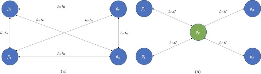
www.nature.com/scientificreports/

                                             Entries      Exits        Time        τ        At,j (τ )   Dt,j (τ )   UtA (τ )       UtD (τ )   Ãt,j (τ )   Ãt,j (τ )
                                             0007328037   0002483731   03:00:00
                                             0007328044   0002483742   07:00:00    0.208      7         11             0            0              7       11
                                             0007328075   0002483781   11:00:00    0.375     31         39             0            4             31       43
                                             0007328193   0002483821   15:00:00    0.542    118         40            0            11         118          51
                                            0007328375    0002483878   19:00:00    0.708    182         57           67             0         249          57
                                            0007328499    0002483910   23:00:00    0.875    124         32          192             0         316          32

                                            Table 1.  An example of the matching process using real data. The columns labelled ENTRIES, EXITS, and
                                            TIME are from the turnstile data. We calculate the number of arrivals, At,j (τ ), by subtracting successive values
                                            of the running total of entries. These arrivals are assigned a fractional time, τ , corresponding to the midpoint
                                            of successive time snapshots. The departures, Dt,j (τ ), are calculated in the same way.

                                            but to the different times at which the number of entries and exits are recorded. We can then write the average
                                            fractional time spent by residents of borough j away from their home borough
                                                                                           ttot
                                                                                       1        k τk At,j (τk ) − Dt,j (τk )
                                                                               �τj =                                           ,                        (7)
                                                                                      ttot                  Mt
                                                                                                  t=1

                                            where ttot is the total number of days. It should be noted that the sum over k is no longer over the number of
                                            riders, but over the number of snapshots of total entries and exits taken that day.
                                                For a variety of reasons, such as travel into and out of the city and the usage of multiple modes of transport,
                                            the number of arrivals and departures at a station will not match exactly. In order to account for this, we match
                                            the number of arrivals and departures at a given snapshot in time in the data, and any discrepancy is added
                                            to the next time bin. Once all time periods have been accounted for, any unmatched arrivals or departures are
                                            ignored. The equation then becomes
                                                                                            ttot
                                                                                        1         k τk min Ãt,j (τk ), D̃t,j (τk )
                                                                              �τj =                                                   ,                     (8)
                                                                                       ttot                   M̃t
                                                                                                  t=1

                                            where

                                                                                           Ãt,j (τk ) = At,j (τk ) + UtA (τk ),                                         (9)

                                                                                           D̃t,j (τk ) = Dt,j (τk ) + UtD (τk ),                                        (10)

                                                                                  UtD (τk ) = max 0, D̃t,j (τk−1 ) − Ãt,j (τk−1 ) ,                                    (11)


                                                                                  UtA (τk ) = max 0, Ãt,j (τk−1 ) − D̃t,j (τk−1 ) ,                                    (12)


                                                                                               UtD (τ0 ) = UtA (τ0 ) = 0,                                               (13)


                                                                                       M̃t = min             At,j (τk ),           Dt,j (τk ) ,                         (14)
                                                                                                        k                      k

                                            where UtA (τk ) and UtD (τk ) are the unmatched arrivals and departures from the previous time period. An example
                                            of the matching process is shown in Table 1. We can now write our mixing parameter
                                                                                                                        Dt,j (τk )
                                                                                         fjj′ (t) = �τj P(dj′ |oj )                           .                         (15)
                                                                                                                                        N
                                                                                                                           k

                                            On any given day we could estimate the number of people, expressed as a fraction of the total population, that
                                                                                               Dt,j (τk )
                                            travel from borough j to borough j′ by P(dj′ |oj ) k           . This would give us an estimate of how many of the
                                                                                                      N
                                            people leaving borough j are heading towards j′ . However, we do not have detailed temporal resolution on the
                                            movement of riders within a borough and we do not know when any individual rider returns to their home
                                            borough. We define an effective population of visitors by multiplying this quantity with �τj , the estimate of the
                                            average time fraction spent away from borough j, that spend the entire day in borough j′ . The mixing parameter
                                            represents this effective visiting population.
                                               The population fraction that leaves region j for all other regions  is fj− = j′ �=j fjj′ , while the population frac-

                                            tion that arrives at region j from all other regions is fj = j′ �=j fj′ j . The resulting total population fraction in
                                                                                                      +
                                            region j becomes pj + fj+ − fj−.

          Scientific Reports |   (2022) 12:6372 |                 https://doi.org/10.1038/s41598-022-10234-8                                                              4

Vol:.(1234567890)
www.nature.com/scientificreports/
We must now keep track of the part of the susceptible and infected populations of region j that do not leave
the region, which we call ’stationary’, given by
S
pj − fj−
sjce = sjce , (16)
pj
S
pj − fj−
ijce = ijce . (17)
pj
It should be noted that while this ’stationary’ population does not leave the borough, the individuals that con-
stitute this population may still be mobile within their borough. This will be addressed later in this section. We
also keep track of infected individuals visiting region j from other regions. These are given by
+
fj′ j
ijce = ij′ ce . (18)
pj′
j ′ � =j
We can now write down the equations for the stationary susceptible and infected populations for region j:
S S S +
sjce (t + �t) = sjce (t)(1 − βjc ijce (t)�t − βjc ijce (t)�t). (19)
We also need to track individuals from region j who are visiting region j′ . These are given by
V
j′
fjj′
sjce = sjce = sjce . (20)
pj
j ′ � =j j ′ � =j
These individuals will interact with stationary infected individuals from other regions. We can now write the
equations for the individuals from region j visiting all other regions
j′
V
sjce (t + �t) = sjce (t)(1 − βj′ c ij+′ ce (t)�t − βj′ c ijS′ ce (t)�t),
(21)
j ′ � =j
We can combine the equations for the stationary and visiting populations by introducing a flow parameter
′
+ j
S
jce =sjS βjc ijce + ijce + sj βj′ c ij+′ ce + ijS′ ce .
(22)
j ′ � =j
The flow parameter lets us compactly write the dynamics of region j
sjce (t + �t) =sjce (t) − jce (t)�t, (23)
(24)
ijce (t + �t) =ijce (t) + jce (t) − ijce (t)γje �t,
rjce (t + �t) =rjce (t) + ijce (t)γje �t. (25)
Since the data provided by the NY government tracks the number of newly reported cases and does not report
the number of active cases (i(t) in our model) we construct the quantity
t+1−�t
new
ijce (t) = jce (t ′ )�t, (26)
t ′ =t
where t is in units of days. In other words, ijce new (t) represents the number of new cases reported on day t and
this is the quantity that we will fit to the data. Figure 2a shows a schematic representation of our mobility-based
SIR model.
Introducing a public transportation node. While our model accounts for the spread of disease through
the transit of infected individuals between regions, it does not take into account that use of public transportation
poses a higher risk of infection3. To account for this effect, we introduce a public transportation node, denoted
by the index T. The fraction of the population permanently residing on this node is 0 ( pT = 0). We modify our
model so that all riders travelling to another borough spend some part of their time at node T. This duration is
taken from the average commute time reported by riders of each b orough21. The mixing parameter from node
j to node T becomes
Dt,j (τk )
fjT (t) = �τjT P(dj′ |oj ) , (27)
N
j ′ � =j k
where �τjT is the commute time for riders in node t, expressed as a fraction of the day. Due to the introduction
of a transport node we must also modify our expression for the inter-borough mixing parameter, which becomes
Scientific Reports | (2022) 12:6372 | https://doi.org/10.1038/s41598-022-10234-8 5
Vol.:(0123456789)www.nature.com/scientificreports/
Figure 2. (a) Schematic representation of the mobility-based SIR model. Each region j has an associated
infection rate βj and mobility parameters fjj′ and fj′ j, which represent individuals from region j visiting region
j′ and vice versa. (b) The enhanced model that includes a public transportation node without a permanent
population. Inter-region mixing still occurs as in the basic model, but the visiting populations of every region
pass through the transportation node for the duration of their commute time during which they are exposed to
the higher infection rate associated with using public transportation. The effective population of region j that is
commuting is given by fjT while the effective population of all other regions that are visiting region j are given
by fj+.
Dt,j (τk )
fjj′ (t) = �τj − �τjT P(dj′ |oj ) . (28)
N
k
Figure 2b shows a schematic depiction of the model with the public transportation node. The introduction of
such a node allows us to independently model the infection rate during rides on public transportation systems,
βT , for individuals using public transportation. Our model does not track individual interactions, but only the
infection rate at the population level. We introduce the transport node to model the different rates of infection
experienced by the fraction of the population that uses the subway, where they interact with a different mixture
of populations than the mixture that they encounter in the boroughs in which they live and work.
Mobility‑dependent infection rate. While inter-region mixing and the introduction of a public trans-
portation node account for mobility between regions, we also need to account for mobility within a region. To do
this, we introduce a mobility parameter for each region, mj (t), which represents the extent to which individuals
are moving within the region. We then write our infection rate as
0
βjce (t) = βjce mj (t),
where βjce
0 is the static infection rate. For the particular case of the NYC subway, m (t) is calculated by taking a
j
7-day moving average of the total trips that start in borough j and rescaling this quantity by dividing it by the
maximum number of trips taken in one day in borough j in this training period, thereby scaling it between 0 and
1. A plot of the average mobility parameter, defined as mavg (t) = j pj mj (t), is plotted in Fig. 4b. We are using
the level of subway usage as a stand-in for all short-range mobility. We found that the number of bike-share rides
taken during the pandemic was correlated with the number of subway t rips19. We assume that subway usage is
correlated with all mobility within the city, even as subway usage fell during the pandemic across cities around
the world27.
Results
While our model is able to incorporate complex demographic information such as healthcare status, access to
testing, and public policies regarding gathering sizes and mask usage, we are limited by the data to which we have
access. Since we only have public transportation data and the daily case count, we will assume that each region
in our model, corresponding to one of the five boroughs of NYC, has a uniform demographic distribution. This
means that we will be ignoring the c and e indices in our model.
In order to model the effect of different policies, we pick March 22, 2020, the official start day of the NY
PAUSE Program, as the beginning of the lockdown. We assume that there are two different infection rates, one
before and the other after this date. This assumption is made because the PAUSE program marks the start of the
implementation of widespread mask usage and social distancing. These are non-mobility factors which impact
the overall infection rate.
We also assume that the intensity of usage of public transportation is correlated with the infection rate. The
infection rate for borough j then becomes
βj (t) = β p (t)mj (t − tD ), (29)
where β p (t) = β h before the start of the NY PAUSE Program on March 22 2020, and β p (t) = β l afterwards. The
second term, mj (t − tD ), represents the normalized daily number of trips taken on the subway within a region.
The parameter tD accounts for the population level delay between subway usage and the subsequent increase in
Scientific Reports | (2022) 12:6372 | https://doi.org/10.1038/s41598-022-10234-8 6
Vol:.(1234567890)www.nature.com/scientificreports/
Figure 3. (a) The best-fit model output of the daily number of new cases in NYC. The black line shows the
model’s output. The red line is the 7-day running average of the total daily reported cases in NYC as a fraction of
the total population of the city. The dotted line indicates the start of the NYC Pause Program. (b) Fitting results
for the model without the mobility-dependent infection rate given by Eq. 29. As the plot demonstrates, we
cannot fit NYC’s COVID-19 spread without modifying the infection rate by the mobility term.
Covid-19 cases. We also average βj (t) over a 7 day moving window in order to smooth out abrupt changes due
to both noise in mj (t) and the discontinuous transition in β p (t).
We have the values of fjj′ (t) and mj (t) from the data, Using these two values, we can construct fjT . We need to
learn the values of β h , β l , γ and τD. We also need to learn the values of βTh and βTl , the infection rate on the subway
before and after the start of the PAUSE program. Figure 3a plots the results of fitting the model by minimizing
the mean squared error (MSE). We fit our model by sweeping over a million values for these parameters, with
our search guided by existing literature on the infection and the recovery r ates28. By contrast, we can see from
Fig. 3b that an SIR model that does not take into account mobility cannot explain the infection trend.
Forecasting. We also masked the last three weeks of data and trained our model without this period. First,
we do a parameter sweep to find the values of the parameters that best fit the training data. Next, we use the end
of the training period, idata
new (t
train ) (where ttrain , is the last day of the training data) as the initial condition for the
testing period. However, we cannot directly use the number of daily new cases as the initial condition. Instead,
the model requires knowledge of the active infected and total recovered cases, i(ttrain ) and r(ttrain ), at the end of
the training period as the initial conditions for the testing period. This was not a concern when we were fitting
our model for the training period since we assumed that i(0) = 1/N and r(0) = 0. In order to predict the spread
of the disease in the testing period, however, we need to know these quantities to serve as the initial conditions
for our model. While data are available for the number of active and recovered cases for New York state, they are
not available for New York City. We estimate the total recovered population by dividing the cumulative deaths
reported in New York City by the state-wide case mortality rate29
Cumulative deaths reported in NYC on day t
rest (t)= , (30)
N ∗ Case mortality rate on day t
where rest (t) is the estimated total recovered population (which includes both individuals who have died as well
as those who have recovered from the disease) expressed as a fraction of the total population of New York City.
We also need to know iest (t), the estimated total active number of infected cases. Specifically, we only need to
estimate iest (ttrain ), the total number of active cases on the last day of the training data. We do this by searching
for a value of iest (ttrain − 1) such that using iest (ttrain − 1) and rest (ttrain − 1) as the initial condition for our model
and predicting the daily number of cases for the next day gives us
inew (ttrain )= idata
new
(ttrain ), (31)
where inew (ttrain ) are the daily number of new cases output by our model on the last day of the training data. The
corresponding values of iest (ttrain ) and rest (ttrain ) become the initial conditions for the model at the start of the
testing period. The model’s prediction is shown in Fig. 4a. Table 2 shows the parameters that minimize the MSE
with and without a testing period.
Discussion
Figure 1a shows that the total number of cases in NYC rapidly increased after the discovery of the first recorded
case, followed by a decline and then a second rise. This trend seems to follow the usage of the subway: initially,
the usage of the subway declines precipitously and then it slowly and partially recovers to about 2/3 of the previ-
ous usage.
Scientific Reports | (2022) 12:6372 | https://doi.org/10.1038/s41598-022-10234-8 7
Vol.:(0123456789)www.nature.com/scientificreports/
Figure 4. (a) The predicted number of daily cases in NYC normalized by the total population of the city. The
red line is the 7-day running average of the total daily reported cases in NYC as a fraction of the total population
of the city. The dashed black line shows the best-fit output of the model in the training period, and the solid
black line shows the model’s prediction for the testing period. The vertical dotted line marks the beginning
of the three-week testing period. The inset figure shows the testing period in more detail. (b) The ratio of the
average infection rate, βavg (t) = j pj βj (t), over the
recovery rate, γ as a function of time. The second axis
shows the average mobility parameter, mavg (t) = j pj mj (t).
Parameter values Data fitting without testing period Data fitting with three-week testing period
βh 1.55 1.59
βl 0.55 0.53
βTh 4 4
βTl 4 4
γ 0.04 0.04
tD 21 days 21 days
Ein 4.46 × 10⁻⁹ 2.98 × 10⁻⁹
Eout – 2.44 × 10⁻¹⁰
2
Rin 0.82 0.88
2
Rout – 0.43
Table 2. The results from fitting the data with and without the last three weeks masked. Ein refers to the MSE
of fitting the data, while Eout shows the MSE of the model’s prediction during the testing period. While we
minimize the MSE during the fitting process, the table also reports the in-sample and out of sample R2 score of
the best fit. We use t = 10−2 for all our simulations.
By scaling our infection parameter with subway usage, we are simultaneously capturing two effects. The first
is the rise in infections directly due to the use of the subway, either through higher infection rate or through
case importation between regions. The second is taking subway usage as a proxy for broader mobility trends,
which in turn depend upon public policy that governs the infection rate. As more people went back to work and
as restrictions on public gatherings, schools etc. were eased, we assume that there was a corresponding increase
in human mobility proportional to the increase in subway usage, even though this usage is just one form of the
total population mobility in the city.
The fact that our model is able to accurately capture both the first wave of infections as well as the second
one indicates that our assumption that subway usage is an indicator for broader human mobility trends (and for
public policies regarding restrictions more generally) within the city is correct. While our model does predict a
higher infection rate for the subway than for the boroughs, infection trends are much less sensitive to inter-region
mobility compared to intra-region mobility.
If we set βj (t) = β p (t) and the dependence on mj (t) is removed, the reduced model is unable to capture the
second wave of infections towards the end of the year as shown in Fig. 3b.
Limitations. The turnstile data that we use imposes some limitations on our model. The most crucial
assumption in our work is that subway usage is correlated to all mobility within the city and can therefore be
used as a proxy for all mobility. This assumption is supported by the fact that the usage of both bikeshares and
Scientific Reports | (2022) 12:6372 | https://doi.org/10.1038/s41598-022-10234-8 8
Vol:.(1234567890)www.nature.com/scientificreports/
taxis dropped at the same time as that of the s ubway19, 20, and bikeshare usage increased in the same period as
subway usage, although at a much faster rate18. Additional data on other forms of mobility, specially in the latter
half of 2020, would allow us to construct the mobility parameter that encapsulates multiple modes of transport.
We also assume that the residents of a borough that leave it using the subway return to the home borough
using the subway on the same day. This assumption impacts our inter-region mixing parameter through the
calculation �τj , the average time spent away from the home borough.
Finally, we assume that the fraction of cases that were reported remained constant throughout 2020. While
we have adjusted for the drop in reporting on the weekends by taking a 7-day moving average, the fraction
of cases that were reported may have changed over the course of the year due to other factors as well. A pos-
sible effect of this variation in the reporting rate is the very high ratio of the average infection rate, defined as
βavg (t) = j pj βj (t), to the recovery rate, γ , that our model predicts during the beginning of the infection, shown
in Fig. 4b. The precipitous rise in cases at the start of the pandemic may represent a slew of people getting tested
in a short amount of time as awareness of the epidemic spread and widespread testing became available, rather
than accurately representing the true spread of the disease. After this initial period our βavg (t)/γ ratio has a
minimum of 1.43 and a maximum of 5.25. While an initial estimate for the reproduction number was reported
to be 2.2 in Wuhan30, other studies using SIR models have reported a much higher reproduction number ranging
from a global estimate of 4.531 to some regions having a value as high as 7.832. While the ratio βavg (t)/γ is not
equivalent to the reproduction number (due to the connectivity of the different compartments in our model)
and should be seen only as a crude estimate, it is encouraging that the ratio predicted by our model falls within
the range of estimates reported in the literature.
Conclusion
The main contribution of this paper is an introduction of a mobility-based model of epidemic spread that uses
a mobility-dependent infection rate. Based only on fitting the data, our model confirms that subway usage is
correlated with the usage of other forms of public transportation because using it as a proxy for the short-range
mobility parameter allows us to predict the two peaks in the NYC infection rate in 2020. Using this model and
the turnstile data from the NYC subway, we predict the trend of daily infections in NYC for a three-week period.
Our model accounts for inter-region mixing of populations, and uses an infection rate that is dependent on the
short-range mobility within a region.
While we have used NYC as a test case, it would be interesting to verify the model with data from other cities.
We believe that by incorporating data from other public transportation services, such as taxis, ride- and bike-
sharing services etc., our model can offer more accurate predictions about the spread of an epidemic disease.
Thus, it can be a useful tool in guiding public policies to tame the spread of pandemics.
Received: 25 July 2021; Accepted: 31 March 2022
References
1. Kraemer, M. U. G. et al. The effect of human mobility and control measures on the COVID-19 epidemic in China. Science
368(6490), 493–497 (2020).
2. Herrera-Valdez, M. A., Cruz-Aponte, M. & Castillo-Chavez, C. Multiple outbreaks for the same pandemic: Local transportation
and social distancing explain the different “waves’’ of A-H1N1pdm cases observed in México during 2009. Math. Biosci. Eng. 8(1),
21–48 (2011).
3. Troko, J. et al. Is public transport a risk factor for acute respiratory infection?. BMC Infect. Dis. 11, 16 (2011).
4. Harris, J. E. The subways seeded the massive coronavirus epidemic in New York City. Working Paper 27021, National Bureau of
Economic Research (April 2020).
5. Fathi-Kazerooni, S., Rojas-Cessa, R., Dong, Z. & Umpaichitra, V. Correlation of subway turnstile entries and COVID-19 incidence
and deaths in New York City. Infect. Dis. Model. 6, 183–194 (2021).
6. Liu, W. et al. Spatiotemporal analysis of Covid-19 outbreaks in Wuhan, China. Sci. Rep. 11(1), 13648 (2021).
7. ...Tian, H. et al. An investigation of transmission control measures during the first 50 days of the COVID-19 epidemic in china.
Science 368(6491), 638–642 (2020).
8. Askitas, N., Tatsiramos, K. & Verheyden, B. Estimating worldwide effects of non-pharmaceutical interventions on Covid-19
incidence and population mobility patterns using a multiple-event study. Sci. Rep. 11(1), 1972 (2021).
9. New York State Department of Health. New York State on PAUSE. https://coronavirus.health.ny.gov/new-york-state-pause.
10. Reichert, T. A. et al. The Japanese experience with vaccinating schoolchildren against influenza. N. Engl. J. Med. 344(12), 889–896
(2001).
11. Carrión, D. et al. Neighborhood-level disparities and subway utilization during the Covid-19 pandemic in New York City. Nat.
Commun. 12(1), 3692 (2021).
12. Kissler, S. M. et al. Reductions in commuting mobility correlate with geographic differences in sars-cov-2 prevalence in New York
City. Nat. Commun. 11(1), 4674 (2020).
13. Verma, R., Yabe, T. & Ukkusuri, S. V. Spatiotemporal contact density explains the disparity of Covid-19 spread in urban neighbor-
hoods. Sci. Rep. 11(1), 10952 (2021).
14. Shi, Y., & Ban, X. Capping mobility to control Covid-19: A collision-based infectious disease transmission model. medRxiv (2020).
15. Meloni, S. et al. Modeling human mobility responses to the large-scale spreading of infectious diseases. Sci. Rep. 1(1), 62 (2011).
16. Metropolitan Transportation Authority. Turnstile data. http://web.mta.info/developers/turnstile.html.
17. New York Governor’s Office. At novel coronavirus briefing, governor cuomo declares state of emergency to contain spread of virus.
https://www.governor.ny.gov/news/novel-coronavirus-briefi ng-governor-cuomo-declares-state-emergency-contain-spread-virus.
18. Wang, H. & Noland, R. B. Bikeshare and subway ridership changes during the Covid-19 pandemic in New York City. Transp. Policy
106, 262–270 (2021).
19. Teixeira, J. F. & Lopes, M. The link between bike sharing and subway use during the COVID-19 pandemic: The case-study of New
York’s Citi bike. Transp. Res. Interdiscip. Perspect. 6, 100166 (2020).
20. Manley, E., Ross, S. & Zhuang, M. Changing demand for New York yellow cabs during the Covid-19 pandemic. Findings 5, 22158
(2021).
Scientific Reports | (2022) 12:6372 | https://doi.org/10.1038/s41598-022-10234-8 9
Vol.:(0123456789)www.nature.com/scientificreports/
21. RSG. Metropolitan Transportation Authority New York City Travel Survey. Technical report, 06 2020.
22. New York City Department of Health and Mental Hygiene. Covid-19: Data. https://www1.nyc.gov/site/doh/covid/covid-19-data.
page.
23. United States Census Bureau. 2020 census. https://data.census.gov/cedsci/ (2020).
24. Kermack, W. O. & McKendrick, A. G. Contributions to the mathematical theory of epidemics-i. Bull. Math. Biol. 53(1), 33–55
(1991).
25. Newman, M. E. J. Networks: An Introduction (Oxford University Press, Oxford, 2010).
26. Mwalili, S., Kimathi, M., Ojiambo, V., Gathungu, D. & Mbogo, R. Seir model for Covid-19 dynamics incorporating the environ-
ment and social distancing. BMC. Res. Notes 13(1), 352 (2020).
27. Wielechowski, M., Czech, K. & Grzeda, Ł. Decline in mobility: Public transport in Poland in the time of the COVID-19 pandemic.
Economies 8(4), 78 (2020).
28. Johansson, M. A. et al. SARS-CoV-2 transmission from people without COVID-19 symptoms. JAMA Netw. Open 4(1), e2035057
(2021).
29. Johns Hopkins University. Covid-19 data repository by the center for systems science and engineering (csse) at Johns Hopkins
University. https://github.com/CSSEGISandData/COVID-19 (2021).
30. Li, Q. et al. Early transmission dynamics in Wuhan, china, of novel coronavirus-infected pneumonia. N. Engl. J. Med. 382(13),
1199–1207 (2020).
31. Katul, G. G., Mrad, A., Bonetti, S., Manoli, G. & Parolari, A. J. Global convergence of Covid-19 basic reproduction number and
estimation from early-time sir dynamics. PLoS ONE 15(9), 1–22 (2020).
32. You, C. et al. Estimation of the time-varying reproduction number of Covid-19 outbreak in china. Int. J. Hyg. Environ. Health 228,
113555–113555 (2020).
Acknowledgements
O.M., G.K., and B.K.S. were supported in part by the Defense Advanced Research Projects Agency (DARPA) and
the Army Research Office (ARO) under Contract No. W911NF-17-C-0099. B.K.S was also supported by ARO
under Contract No. W911NF-16-1-05241. The views and conclusions contained in this document are those of
the authors and should not be interpreted as representing the official policies either expressed or implied by the
U.S. Government.
Author contributions
B.K.S and O.M. conceived the research and extended the SIR model to include impact of short-term trips. A.M.
collected and initially processed NYC subway mobility data. O.M. wrote the model simulation. O.M., B.G. and
A.M. analyzed the data. O.M., B.G., A.M., G.K., and B.K.S. discussed results. O.M and B.G. wrote the paper with
input from all authors.
Competing interests
The authors declare no competing interests.
Additional information
Correspondence and requests for materials should be addressed to O.M.
Reprints and permissions information is available at www.nature.com/reprints.
Publisher’s note Springer Nature remains neutral with regard to jurisdictional claims in published maps and
institutional affiliations.
Open Access This article is licensed under a Creative Commons Attribution 4.0 International
License, which permits use, sharing, adaptation, distribution and reproduction in any medium or
format, as long as you give appropriate credit to the original author(s) and the source, provide a link to the
Creative Commons licence, and indicate if changes were made. The images or other third party material in this
article are included in the article’s Creative Commons licence, unless indicated otherwise in a credit line to the
material. If material is not included in the article’s Creative Commons licence and your intended use is not
permitted by statutory regulation or exceeds the permitted use, you will need to obtain permission directly from
the copyright holder. To view a copy of this licence, visit http://creativecommons.org/licenses/by/4.0/.
© The Author(s) 2022
Scientific Reports | (2022) 12:6372 | https://doi.org/10.1038/s41598-022-10234-8 10
Vol:.(1234567890)You can also read