Modelling supraglacial debris-cover evolution from the single-glacier to the regional scale: an application to High Mountain Asia
←
→
Page content transcription
If your browser does not render page correctly, please read the page content below
The Cryosphere, 16, 1697–1718, 2022
https://doi.org/10.5194/tc-16-1697-2022
© Author(s) 2022. This work is distributed under
the Creative Commons Attribution 4.0 License.

Modelling supraglacial debris-cover evolution from the
single-glacier to the regional scale: an application to
High Mountain Asia
Loris Compagno1,2 , Matthias Huss1,2,3 , Evan Stewart Miles2 , Michael James McCarthy2 , Harry Zekollari4,5,1,2 ,
Amaury Dehecq1,2 , Francesca Pellicciotti2 , and Daniel Farinotti1,2
1 Laboratory of Hydraulics, Hydrology and Glaciology (VAW), ETH Zurich, Zurich, Switzerland
2 Swiss Federal Institute for Forest, Snow and Landscape Research (WSL), Birmensdorf, Switzerland
3 Department of Geosciences, University of Fribourg, Fribourg, Switzerland
4 Department of Geoscience and Remote Sensing, Delft University of Technology, Delft, the Netherlands
5 Laboratoire de Glaciologie, Université libre de Bruxelles, Brussels, Belgium

Correspondence: Loris Compagno (compagno@vaw.baug.ethz.ch)

Received: 4 August 2021 – Discussion started: 27 August 2021
Revised: 29 March 2022 – Accepted: 1 April 2022 – Published: 6 May 2022

Abstract. Currently, about 12 %–13 % of High Mountain               fraction is expected to increase, while mean debris thickness
Asia’s glacier area is debris-covered, which alters its sur-        is projected to show only minor changes, although large lo-
face mass balance. However, in regional-scale modelling             cal thickening is expected. To isolate the influence of explic-
approaches, debris-covered glaciers are typically treated as        itly accounting for supraglacial debris cover, we re-compute
clean-ice glaciers, leading to a bias when modelling their fu-      glacier evolution without the debris-cover module. We show
ture evolution. Here, we present a new approach for mod-            that glacier geometry, area, volume, and flow velocity evolve
elling debris area and thickness evolution, applicable from         differently, especially at the level of individual glaciers. This
single glaciers to the global scale. We derive a parameteri-        highlights the importance of accounting for debris cover and
zation and implement it as a module into the Global Glacier         its spatiotemporal evolution when projecting future glacier
Evolution Model (GloGEMflow), a combined mass-balance               changes.
ice-flow model. The module is initialized with both glacier-
specific observations of the debris’ spatial distribution and
estimates of debris thickness. These data sets account for the
fact that debris can either enhance or reduce surface melt de-      1   Introduction
pending on thickness. Our model approach also enables rep-
resenting the spatiotemporal evolution of debris extent and         In High Mountain Asia (HMA), debris-covered and clean-
thickness. We calibrate and evaluate the module on a se-            ice glaciers are losing mass due to climate change (Brun
lected subset of glaciers and apply GloGEMflow using dif-           et al., 2017; Zemp et al., 2019; Shean et al., 2020; Hugonnet
ferent climate scenarios to project the future evolution of all     et al., 2021). Since the atmosphere is expected to warm fur-
glaciers in High Mountain Asia until 2100. Explicitly ac-           ther (Lee et al., 2021), more glacier mass is expected to be
counting for debris cover has only a minor effect on the pro-       lost (Marzeion et al., 2020; Rounce et al., 2020). Understand-
jected mass loss, which is in line with previous projections.       ing how sensitive HMA glaciers are to changes in climate is
Despite this small effect, we argue that the improved pro-          crucial to quantify the future glacier evolution in the area.
cess representation is of added value when aiming at captur-           A key unknown is the present and future influence of
ing intra-glacier scales, i.e. spatial mass-balance distribution.   supraglacial debris cover in moderating melt rates for the
Depending on the climate scenario, the mean debris-cover            12 %–13 % of HMA’s glacier area that is presently covered
                                                                    by debris (Herreid and Pellicciotti, 2020). A better under-

Published by Copernicus Publications on behalf of the European Geosciences Union.
1698                                                    L. Compagno et al.: Regional-scale modelling of supraglacial debris

standing is necessary to accurately predict future water avail-       By combining estimates of sub-debris melt with surface
ability; to assess impacts on irrigation, hydropower, and both     temperature inversion methods, Rounce et al. (2021) re-
public and private usage of water (Biemans et al., 2019;           cently presented the first global estimate of supraglacial de-
Farinotti et al., 2019b; Fyffe et al., 2019; Immerzeel et al.,     bris thickness distribution on glaciers. The estimate refers
2020; Miles et al., 2021); to anticipate hotspots of hazards       to about 2008, but debris thickness evolves through time.
such as ice-dammed or proglacial lakes (Emmer et al., 2014;        The few direct observations available indicate a debris-cover
Zheng et al., 2021); or to project the glaciers’ contribution to   thickening in the last decades (e.g. Gibson et al., 2017; Ver-
sea-level rise (Edwards et al., 2021).                             haegen et al., 2020), most probably related to the negative
   The presence of debris at the ice surface has the effect of     mass balances induced by ongoing climate change as well
reducing the surface albedo and increasing the net short-wave      as to the resulting glacier thinning and decelerated ice flow
radiation (Owen et al., 2003; Reid and Brock, 2010). When          (Verhaegen et al., 2020; Anderson et al., 2021a). Supraglacial
debris is particularly thin and/or patchy, this excess energy      ice cliffs and ponds might additionally contribute to this, as
can be readily conducted to the ice, thus enhancing melt rates     they enhance local ablation of debris-covered glaciers (Sakai
(Østrem, 1959; Reznichenko et al., 2010a; Fyffe et al., 2020).     et al., 2000, 1998; Ragettli et al., 2016; Miles et al., 2018)
However, for thicker, continuous debris layers, the increased      and evolve as well (Narama et al., 2017; Watson et al., 2017;
isolation layer allows for high debris surface temperatures        Chand and Watanabe, 2019; Buri et al., 2021; Ferguson and
(often > 15 ◦ C), thereby increasing both the outgoing long-       Vieli, 2021).
wave radiation and the turbulent energy fluxes directed away          Regional and global models with various levels of com-
from the surface (e.g. Nicholson and Benn, 2006; Steiner           plexity have been used to simulate HMA’s future glacier
et al., 2018). This results in a reduced and delayed conduc-       evolution (see Marzeion et al., 2020, for a model inter-
tion of energy to the glacier ice, leading to a progressive re-    comparison). The models use different methodologies for
duction in melt with increasing debris thickness (e.g. Østrem,     computing ablation, accumulation, or geometry changes but
1959; Reznichenko et al., 2010a; Anderson and Anderson,            rarely take into account the debris cover and its spatiotem-
2016; Rounce et al., 2021).                                        poral evolution. An exception is the study by Kraaijenbrink
   Since glaciers are presently far from equilibrium               et al. (2017) that presented the first HMA glacier projec-
(Marzeion et al., 2018; Zekollari et al., 2020; Miles et al.,      tions explicitly accounting for the effect of supraglacial de-
2021), their debris cover is evolving through time (Stokes         bris. However, the study neither considered an evolution of
et al., 2007; Bhambri et al., 2011; Bolch et al., 2011; Shukla     debris extent and thickness in the future nor modelled ice
and Qadir, 2016; Tielidze et al., 2020). Indeed, medial            flow explicitly or used glacier-specific mass-balance data for
moraines and debris patches – which are formed by the ac-          calibration. Glacier-specific studies considering debris-cover
cumulation and transport of debris – tend to grow and to ex-       evolution exist (e.g. Jouvet et al., 2011; Rowan et al., 2015;
pand laterally with increasing ablation (Anderson, 2000; Jou-      Kienholz et al., 2017; Scherler and Egholm, 2020; Verhae-
vet et al., 2011; Rowan et al., 2015; Kienholz et al., 2017;       gen et al., 2020), as well as theoretical and process-based
Wirbel et al., 2018; Verhaegen et al., 2020). Additionally,        modelling studies (Anderson and Anderson, 2016; Ferguson
ice-marginal moraines, which may become unstable when              and Vieli, 2021), but the majority are based on higher-order
glaciers retreat, can supply the ice surface with additional de-   ice-flow models and require rather extensive observational
bris (Van Woerkom et al., 2019). As a consequence, glaciers        data. Thus, the corresponding methods are hardly applicable
with negative mass balances tend to increase their debris-         at larger scales.
cover fractions through time (Stokes et al., 2007; Bhambri            Here, we present a new debris area and thickness evolu-
et al., 2011; Bolch et al., 2011; Shukla and Qadir, 2016;          tion module applicable to both individual glaciers and the
Tielidze et al., 2020). In the Karakoram region, instead, pos-     regional to global scale. The module is included into the
itive and negative debris-cover changes have offset one an-        Global Glacier Evolution Model (GloGEMflow), a combined
other during the past 40 years (Herreid et al., 2015). This is     mass-balance (Huss and Hock, 2015) ice-flow (Zekollari
most probably the consequence of the neutral or even slightly      et al., 2019) model. We calibrate and extensively evaluate
positive mass balance in the region (Gardelle et al., 2013;        the debris-cover module and showcase its applicability for all
Farinotti et al., 2020).                                           glaciers in High Mountain Asia. We focus on the future evo-
   For glaciers with negative mass balances, the debris also       lution of debris cover and determine the impacts that explic-
progressively expands up-glacier (Stokes et al., 2007), to-        itly modelling debris-cover evolution has on transient glacier
gether with the rise in the equilibrium line altitude (ELA).       evolution. To do so, we model all HMA glaciers between
Indeed, the mass-balance profile of a debris-covered glacier       2000 and 2100. The modelling is based on five Shared So-
may have a local minimum at mid-elevations, especially if          cioeconomic Pathways (SSP119, SSP126, SSP245, SSP370,
the ice is clean (i.e. not covered by debris) at that eleva-       and SSP585) from the sixth phase of the Coupled Model
tion. This fosters the expansion of the debris-cover fraction      Intercomparison Project (CMIP6), and the results are com-
through the melt-out of englacial debris transported by the        pared to model runs that do not explicitly account for debris
glacier’s ice flow (Stokes et al., 2007; Rowan et al., 2015).      cover. We discuss the resulting differences in terms of glacier

The Cryosphere, 16, 1697–1718, 2022                                                   https://doi.org/10.5194/tc-16-1697-2022
L. Compagno et al.: Regional-scale modelling of supraglacial debris                                                          1699

mass balance, glacier evolution, and ice-flow velocity, which       based nature of the procedure, the energy-balance model and
allows us to assess the importance of accounting for debris-        the Østrem curves (see below) are not explicitly calibrated
cover evolution in regional studies.                                but use model parameter that are based on literature values.
                                                                    The debris thickness maps are evaluated using a large amount
                                                                    of available in situ data (148 007 data points on 13 glaciers)
2     Data                                                          on debris thickness, showing good agreement (see McCarthy
                                                                    et al., 2021). To model surface mass balance, the energy-
To model the evolution all 95 536 glaciers contained in the         balance model was run at randomly chosen points on the sur-
Randolph Glacier Inventory version 6.0 (RGI 6.0; RGI Con-           face of each glacier and with randomly chosen debris thick-
sortium, 2017) for HMA over the 21st century, different data        nesses and debris properties within expected physical ranges.
sets are used (see Fig. 1).                                         To generate the Østrem curves, in a first step, the energy-
                                                                    balance model was run at randomly chosen points on the sur-
2.1    Glacier geometry
                                                                    face of each considered glacier and with debris thicknesses
We use glacier outlines from RGI 6.0 (RGI Consortium,               and debris properties randomly chosen within expected phys-
2017), which is a global inventory of glacier outlines. For         ical ranges. These Østrem curves are expressed as
HMA glaciers, the RGI outlines are based on remote sensing               idebris · kdebris
data acquired between 1998 and 2013. For the ice thickness,         b=                     ,                                   (1)
                                                                           h + kdebris
we use the consensus estimate by Farinotti et al. (2019a),
which is based on an ensemble of models using characteris-          where b is the local surface mass balance (m w.e. a−1 ), h is
tics of the glacier surface (e.g. slope and surface velocities)     the debris thickness (m), and idebris (m w.e. a−1 ) and kdebris
and principles of ice-flow dynamics for ice thickness inver-        (m) are glacier-specific calibration parameters without spe-
sion. For the modelling, the geometry is simplified by sub-         cific physical meaning. The mean and 95 % confidence inter-
dividing each glacier into elevation bands of 10 m, includ-         val for idebris are −1.86 and [−7.62, −0.09], respectively. For
ing tributary glaciers (Huss and Hock, 2015) (i.e. they are         kdebris the equivalent values are 0.10 and [0.01, 0.22]. Note
not treated separately). In this elevation-dependent represen-      that Eq. (1) has similarities with the hyper-fit model of An-
tation, the transversal glacier bed shape is parameterized as-      derson and Anderson (2016) and Anderson et al. (2021a, b),
suming a glacier cross-section that has the form of an isosce-      although we note that the two approaches differ in the num-
les trapezoid with 45◦ base angles (see Zekollari et al., 2019,     ber of parameters and their interpretation. In a second step,
for more details).                                                  the mass balances inferred by Miles et al. (2021) were used
                                                                    together with the fitted Østrem curves (Eq. 1) for each el-
2.2    Debris cover and Østrem curves                               evation (i.e. assuming that englacial and basal mass bal-
                                                                    ance is negligible) to determine the debris thickness maps
For each glacier with an area > 2 km2 with debris cover             used in this study. The so-obtained information represents
(i.e. 6115 glaciers in total; see RGI Consortium, 2017), the        the supraglacial debris conditions for the period 2000–2016.
debris coverage is represented by a debris-cover mask gener-        With the method described above, McCarthy et al. (2021) es-
ated using Landsat scenes acquired between 2013 and 2017            timate a mean debris thickness for the debris-covered part of
(Scherler et al., 2018), as well as spatially distributed debris-   all glaciers in HMA of 0.34 m (with an uncertainty between
cover thickness maps and glacier-specific Østrem curves             0.15 and 0.76 m). The uncertainties are asymmetric because
(i.e. a function that characterizes the relation between debris-    surface mass balance is less sensitive to debris thickness as
cover thicknesses and melt rates; Østrem, 1959).                    debris thickness increases and are in line with other stud-
   The debris thickness maps are based on McCarthy et al.           ies (e.g. Rounce et al., 2021). For our purposes, the spatially
(2021), who used a simplified surface mass-balance inver-           distributed debris-cover information is divided into elevation
sion procedure similar to Ragettli et al. (2015) and Rounce         bands of 10 m, whilst the Østrem curves were directly added
et al. (2018). In a nutshell, the procedure uses the principle      into our mass-balance module (see Sect. 3.1).
of mass conservation to infer local glacier mass balance from          To calibrate and evaluate the parameterizations used for
surface velocities and thinning rates and then iteratively ad-      describing the evolution of both debris area and thickness
justs the debris thickness to ensure consistency between the        (see Sect. 3.2), we use multiple Hexagon and Landsat satel-
so-inferred mass balance and the output of an energy-balance        lite images acquired between 1973–1976 and 1987–2019, re-
model driven by meteorological data. More specifically, the         spectively. The Hexagon images (Maurer and Rupper, 2015),
procedure uses digital elevation models (DEMs), glacier ice         available as scan of raw film images from the US Geologi-
thickness, surface velocity, debris proprieties, and meteoro-       cal Survey, were georeferenced and orthorectified following
logical forcing data as input and uses them to calculate ice        the methodology of Dehecq et al. (2020). Since the Hexagon
flux divergence and ice thinning rates. The debris thickness        images are monochromatic, debris cover has been delineated
is then adjusted until modelled and observed ice-melt rates         manually for 31 glaciers distributed through HMA. We use
agree within a prescribed tolerance. Due to the physically          glaciers with sufficient contrast between debris and clean ice,

https://doi.org/10.5194/tc-16-1697-2022                                                        The Cryosphere, 16, 1697–1718, 2022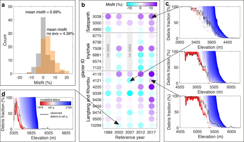
1700                                                        L. Compagno et al.: Regional-scale modelling of supraglacial debris

Figure 1. (a) Extent of HMA glaciers (white) as per Randolph Glacier Inventory version 6 (RGI; RGI Consortium, 2017). The three main
RGI regions (Central Asia, South Asia West, and South Asia East) are shown by blueish, reddish, and greenish colours, respectively. RGI
second-order regions are labelled individually. Three glaciers are highlighted to illustrate glacier-specific model results (red circles with
numbers). (b, c, d) Map of the three highlighted glaciers with their mean 2000–2016 debris thickness given by colours (scale in panel b).
Glacier outlines and debris thickness are from RGI Consortium (2017) and McCarthy et al. (2021), respectively. For each glacier, V is the
glacier ice volume according to Farinotti et al. (2019a); A is the glacier area according to RGI 6.0; Adebris is the debris-covered area; and
hdebris is the mean debris-cover thickness with superscript and subscript values indicating its estimated confidence interval (note that the
latter is not symmetric; cf. Sect. 2.2). (e, f, g) Glacier hypsometry (area per 10 m elevation band) and debris-covered area distribution at
inventory date; n is the number of glaciers within each region (RGI Consortium, 2017). Map background source: Natural Earth.

little to absent shadows on the glacier surface, and with-               2004–2009, 2010–2014, and 2015–2019. Each multi-date
out snow on the ablation zone. For the Landsat satellite im-             composite is visually checked, then a debris–ice transition
ages, debris is identified automatically following the multi-            threshold is chosen automatically with an Otsu routine (Otsu,
date composite approach of Scherler et al. (2018). We apply              1979). By using images stemming from different epochs and
this method to the combined multi-sensor Landsat archive                 through suitable selection (see Sect. 3.2), the area covered by
in Google Earth Engine for additional epochs with sufficient             debris is identified for 68 glaciers, again scattered throughout
Landsat acquisitions: 1987–1991, 1994–1999, 1999–2003,                   HMA. All 31 glaciers for which debris cover is identified on

The Cryosphere, 16, 1697–1718, 2022                                                           https://doi.org/10.5194/tc-16-1697-2022
L. Compagno et al.: Regional-scale modelling of supraglacial debris                                                            1701

the Hexagon images are also covered by the Landsat data. All       ules (i.e. the ones dealing with mass balance, ice flow, and
glaciers are divided into two sets. The first set (termed S1) is   debris cover) are presented.
composed of 55 glaciers where debris is identified on Land-
sat images and 18 glaciers where the debris is identified from     3.1   Mass balance
Hexagon imagery. The second set (termed S2) is composed
of 11 glaciers where debris is identified on both Landsat and      Accumulation is computed by summing solid precipitation,
Hexagon images. This division into two sets is done to en-         which is determined by applying a local temperature thresh-
sure independence between data used in the calibration and         old of 1.5 ◦ C (with a linear transition between liquid and
the evaluation of the debris-evolution module.                     solid precipitation in the 0.5 and 2.5 ◦ C range) to the ERA5
                                                                   grid cell closest to the glacier. To account for the precipitation
2.3    Mass balance                                                increase with elevation, we apply a lapse rate of 0.015 % m−1
                                                                   (for consistency, it is the same as Huss and Hock, 2015). For
To calibrate the mass-balance module of GloGEMflow, we             glaciers with an elevation range over 1000 m, precipitation is
rely on glacier-wide geodetic volume changes available for         reduced in the uppermost quarter with an exponential func-
2000–2019 (Hugonnet et al., 2021). These volume changes            tion to account for reduced moisture content in the air and
were obtained from surface-elevation changes determined by         stronger wind erosion (see Huss and Hock, 2015, for details).
using stereo images from the Advanced Spaceborne Thermal              A degree-day model (Hock, 2003) is used to compute ab-
Emission and Reflection Radiometer (ASTER). The volume             lation. Ice, firn, and snow are differentiated by using a dif-
changes are converted into mass changes by using a con-            ferent degree-day factor (DDF), with a ratio between DDFice
stant density conversion factor of 850 kg m−3 (Huss, 2013).        and DDFsnow of 2.0 and a ratio between DDFice and DDFfirn
The data set provides a volume change estimate for all in-         of 1.5. The air temperature lapse rate, used to determine
dividual glaciers. It covers ∼ 99.8 % of the regional glacier      temperature for each elevation band of the glacier surface,
area (Hugonnet et al., 2021). For the remaining ∼ 0.2 %, data      is computed from temperature fields at distinct geopotential
from a nearby glacier are chosen by following the same pro-        heights provided by the ERA5 data set (see Compagno et al.,
cedure as described in Compagno et al. (2021). To evaluate         2021, for more details).
the mass-balance module, we use independent data from in              For debris-covered ice, melt enhancement and reduction
situ observations provided by the World Glacier Monitoring         due to thin and thick debris cover, respectively, are accounted
Service for 21 glaciers (WGMS, 2020).                              for. This is done by applying a glacier-specific Østrem curve
                                                                   (see Sect. 2.2) that relates ablation (a) under debris to debris
2.4    Climate                                                     thickness (h) using Eq. (1), while the standard GloGEMflow-
                                                                   calculated ablation (without debris) is used for h = 0. In Glo-
For forcing GloGEMflow between 1979 and 2020, we use               GEMflow, the relation between ablation and debris cover is
2 m temperature and precipitation data of the European             applied to each elevation z and each time step t and can be
Centre for Medium-Range Weather Forecasts Reanalysis               expressed as
(ERA5) (Hersbach et al., 2019). For the future (2020–2100),        (
                                                                       debris = a · g
                                                                     az,t                    if g < 1.65,
we use 53 members of the CMIP6 ensemble (Eyring et al.,                          z,t
                                                                       debris
                                                                                                                                  (2)
2016) from 12 different general circulation models (GCMs),           az,t = az,t · 1.65 if g > 1.65,
covering 5 SSPs (5 members for SSP119 and 12 members for
                                                                   where az,tdebris (m w.e. a−1 ) is ablation of debris-covered ice
all other SSPs). Both data sets have a monthly resolution. To
ensure consistency between past and future, a de-biasing pro-      and az,t (m w.e. a−1 ) is ablation of bare ice at elevation z and
cedure is applied that adjusts the GCMs to the ERA5 data set       time t. The factor g (which acts as a factor enhancing ab-
(see Huss and Hock, 2015, for details). This procedure ap-         lation due to debris) depends on debris-cover thickness hz,t
plies a set of additive and multiplicative corrections to adjust   (m) and the glacier-specific parameter kdebris (see Eq. 1), used
the long-term mean difference and the short-term variability       by McCarthy et al. (2021) to fit the Østrem curve; g can be
in the coarse-resolution GCMs (with a horizontal resolution        expressed as follows:
of about 100 km) to the high-resolution ERA5 data (with a               ( (k
                                                                            debris +hcrit )
horizontal resolution of about 30 km).                                                      ,                if hz,t > heff ,
                                                                   g = (khdebris
                                                                             z,t +kdebris
                                                                                   +hcrit ) hz,t  heff −hz,t                      (3)
                                                                           heff +kdebris · heff +    heff , if hz,t < heff ,

3     Methods                                                      where hcrit is the critical debris thickness (m), i.e. the debris
                                                                   thickness for which ice melt beneath debris is identical to the
GloGEMflow is a combined mass-balance and ice-flow                 melt of bare ice (Reznichenko et al., 2010b) and heff is the de-
model, extended with a new component for debris-cover evo-         bris thickness for which the enhancement of melt is maximal.
lution for this study. The general workflow of this study is       Here, we use hcrit = 0.036 m and heff = 0.016 m, which are
illustrated in Fig. 2. In the following sections, the three mod-   the means for hcrit and heff as determined from observations

https://doi.org/10.5194/tc-16-1697-2022                                                  The Cryosphere, 16, 1697–1718, 2022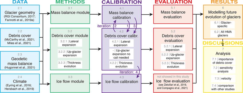
1702 L. Compagno et al.: Regional-scale modelling of supraglacial debris
Figure 2. Study overview. The grey numbers correspond to the sections of this paper. The “METHODS” column also depicts the different
modules included in GloGEMflow. The violet arrows show the iterations between the modules during the calibration.
by 11 local studies across HMA (Khan, 1989; Mattson and 3.2.1 Lateral expansion of debris cover
Gardner, 1989; Kayastha et al., 2000; Tangborn and Rana,
2000; Mihalcea et al., 2006; Hagg et al., 2008; Wei et al., The lateral expansion of an already existing debris layer
2010; Dobhal et al., 2013; Juen et al., 2014; Sharma et al., (e.g. medial and ice-marginal moraines, as well as isolated
2016; Groos et al., 2018; see Table S1 in the Supplement). debris patches) is linked to the local mass balance (Stokes
In Eq. (2), g is constrained to a maximal value of 1.65, et al., 2007; Bhambri et al., 2011; Bolch et al., 2011; Shukla
which corresponds to the highest observed melt enhancement and Qadir, 2016; Tielidze et al., 2020). We describe the pro-
factor reported in the 11 local studies (see Table S1). For cess of lateral expansion on a yearly time step by
glacier-specific Østrem curves and examples of hcrit and heff ,
see Figs. 3 and S1 in the Supplement. γz,t = γz,t−1 + abs(bz,t ) · B(t−9,t) · (−1) · γz,t−1
· clateral , if z < ELA, (4)
3.2 Debris-cover evolution
where γz,t is the fraction of debris cover in elevation band z
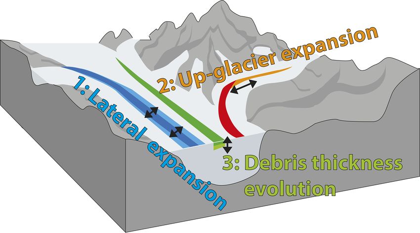
The evolution of debris-cover extent and thickness is parame- at time t, bz,t is the mass balance at elevation z at time t,
terized by accounting for three main processes: (1) the lateral and B(t−9,t) is the 10-year moving average of the glacier-
expansion of debris cover within individual elevation bands, wide mass balance, evaluated between years t − 9 and t;
which is meant to mimic the observed lateral expansion of clateral is a regional debris-cover extension parameter which
medial moraines and debris patches; (2) the debris up-glacier is calibrated to minimize the difference between observed
expansion, which describes the progressive appearance of de- and computed lateral expansion of debris (see Sect. 4.2). The
bris at higher elevation when the ELA rises; and (3) debris first term of Eq. (4) accounts for pre-existing debris cover,
thickness evolution, which accounts for the progressive accu- while the second term describes the rate of debris expansion.
mulation of debris on the surface due to insufficient export by The latter is proportional to the local mass balance abs(bz,t ),
ice flow (see Fig. 4). Note that ponds and ice cliffs, known to which is generally negative where debris cover is present,
influence the surface mass balance of debris-covered glaciers thus accounting for the expected increase in lateral debris for
as well (Ragettli et al., 2016; Miles et al., 2018; Rounce et al., locations with higher melt rates (Jouvet et al., 2011; Stokes
2018), are implicitly accounted for during the Østrem curve et al., 2007; Bhambri et al., 2011; Bolch et al., 2011; Shukla
fitting procedure (see Sect. 2.2), since their effect is already and Qadir, 2016; Tielidze et al., 2020).
accounted for in the mass-balance data (Miles et al., 2021). We also consider debris expansion to be inversely propor-
We do not model ponds and ice cliffs explicitly because (1) of tional to the 10-year moving average of glacier-wide mass
the lack of detailed information that would be needed for balance B(t−9,t) . By doing so, we parametrize ice-dynamical
accurate calibration and evaluation at the regional scale and processes: in the case of negative long-term mass balance,
(2) their long-term and future evolution is uncertain (Narama the debris-cover fraction increases, resulting in an accumula-
et al., 2017; Watson et al., 2017; Chand and Watanabe, 2019; tion of debris; in the case of positive long-term mass balance,
Mölg et al., 2020) and requires small-scale, specific process the debris fraction decreases, mimicking debris evacuation
models to be captured (e.g. Buri et al., 2021; Kneib et al., by ice flow (Anderson and Anderson, 2016; Ferguson and
2021). Vieli, 2021); and in case of neutral long-term mass balance,
The Cryosphere, 16, 1697–1718, 2022 https://doi.org/10.5194/tc-16-1697-2022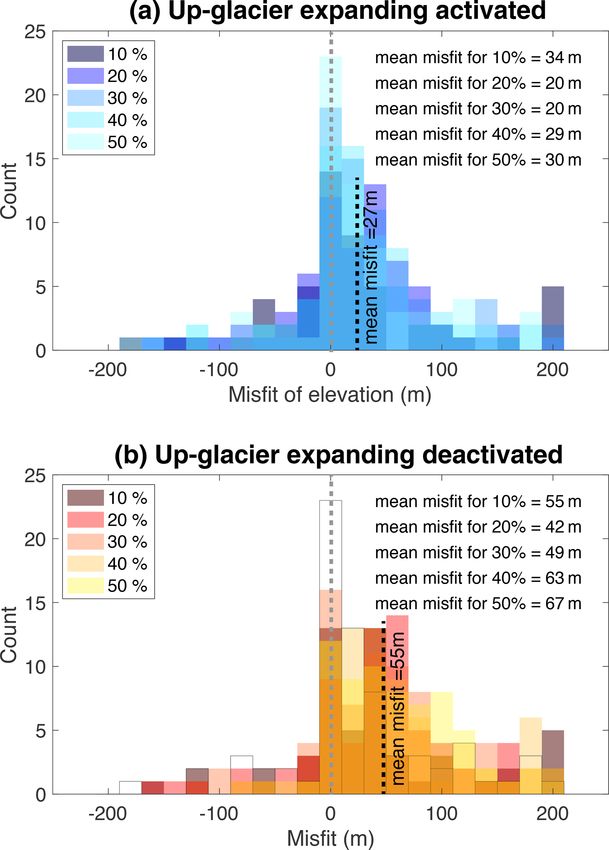
L. Compagno et al.: Regional-scale modelling of supraglacial debris                                                                      1703

Figure 3. Schematic of the melt enhancement factor g (dimensionless) as a function of debris thickness for three different glaciers (green
lines; k is the value of kdebris calibrated for each glacier). The coloured, dashed boxes show regions in which the different cases of Eqs. (2)
and (3) apply. MB: mass balance.

                                                                          only applied in the glacier ablation zone. Debris cover is not
                                                                          permitted in the accumulation zone.

                                                                          3.2.2    Up-glacier expansion of debris cover

                                                                          For glaciers with negative mass balances, debris cover has
                                                                          been observed to progressively expand up-glacier (Deline
                                                                          and Orombelli, 2005; Stokes et al., 2007). We assume that
                                                                          this is related to the rise in the ELA and in the melt-out of
                                                                          debris in areas that transit from the accumulation to the abla-
                                                                          tion zone (Anderson, 2000). As Eq. (4) does not permit sim-
Figure 4. Sketch showing the three main processes (parameteriza-          ulating the expansion of debris to new elevation bands, we
tions) captured by the debris-cover extent and thickness evolution        parameterize this process as
module.
                                                                                 γz−1,t + γz+1,t
                                                                          γz,t =                 , if γz,t−1 = 0
                                                                                        2
                                                                                                 dELAt−9,t
                                                                              and z < ELA and               > 0.                           (5)
                                                                                                    dt
the debris fraction remains stable. Such a neutral up to posi-
tive evolution has for example been observed in the Karako-               This process is discretized within elevation bands of 10 m.
ram over the last 40 years (Herreid et al., 2015). Since there            The number of elevation bands h without debris at time t − 1
are not enough observational data that would allow for con-               that can gain debris from a nearby elevation band at time t
straining the parameter, the time window of 10 years, which               (we use yearly time steps) applying Eq. (5) is equal to the
accounts for the time it takes for the debris cover of a glacier          rise in the ELA over the last 10 years, determined using linear
to respond to changes in the glacier-wide mass balance, is                regression of the values (ELA(t−9,t) ), i.e.
based on judgement. Our implementation also accounts for
                                                                                  dELAt−9,t
the observation that in elevations with limited debris, rela-             #h =              .                                              (6)
tive expansion is slower compared to elevations with a high                         dt · 10
debris fraction. Small debris fractions are often associated                 In other words, the up-glacier expansion of debris cover
with small moraines or isolated debris patches, indicative of             rises with the ELA rise. The thickness of new debris is arbi-
relatively limited debris concentration in the ice. Areas with            trarily set to 1 cm. If the slope of the above linear regression
abundant debris cover may grow faster due to enhanced de-                 is zero or negative, Eq. (5) is not applied. With the above pro-
bris supply from melt-out or due to ice-flow changes (Ander-              cess, debris migrates towards higher elevations at the same
son, 2000; Anderson et al., 2021b). Note that this equation is            rate as the ELA rises. If the ELA does not rise, the maximal

https://doi.org/10.5194/tc-16-1697-2022                                                          The Cryosphere, 16, 1697–1718, 2022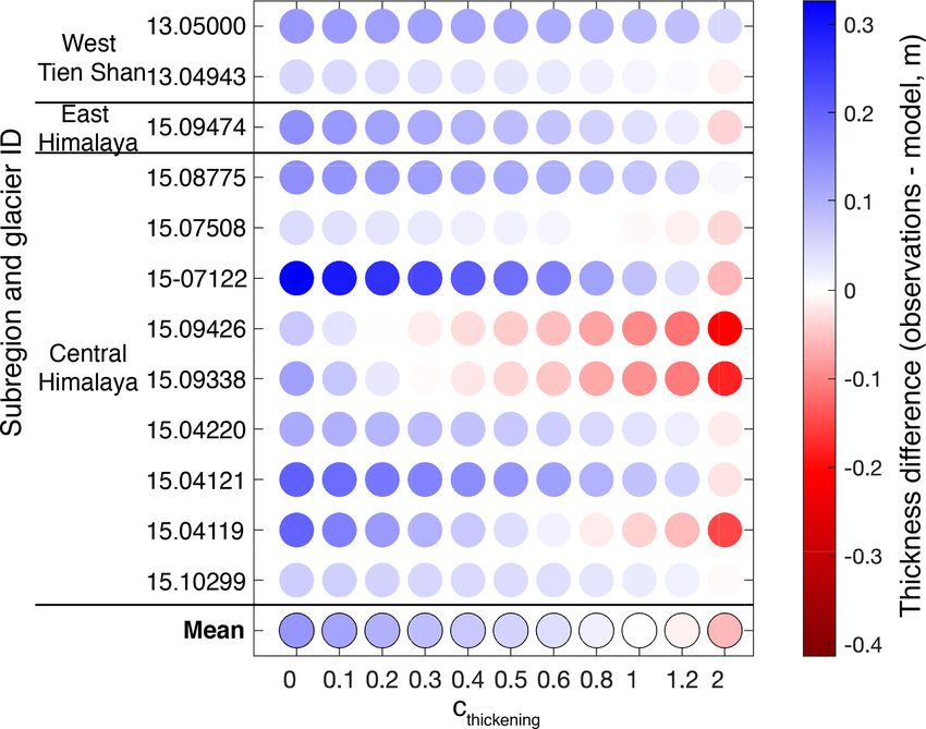
1704                                                    L. Compagno et al.: Regional-scale modelling of supraglacial debris

elevation at which debris is encountered will remain stable        for details). This is done for all glaciers with an area > 2 km2 ,
or decrease if the glacier mass balance is positive, e.g. due to   with the ice flow being controlled by a deformation-sliding
negative lateral expansion of debris cover (see Sect. 3.2.1).      factor that accounts for both internal ice deformation and
The procedure was not calibrated due to the need of a con-         basal sliding. This deformation-sliding factor is calibrated
siderable amount of accurate data. An evaluation of the per-       for each glacier specifically (see Sect. 4.3). For all glaciers
formance is found in Sect. 5.2.2.                                  with an area < 2 km2 , glacier evolution is modelled with an
                                                                   elevation-dependent parameterization, which was shown to
3.2.3    Debris thickness evolution                                be in good agreement with results from higher-order ice-flow
                                                                   models (Huss et al., 2010).
As for the lateral expansion of debris, the evolution of de-
bris thickness is linked to internal debris concentration and
glacier mass balance (e.g. Gibson et al., 2017; Mölg et al.,
                                                                   4     Model calibration
2019; Verhaegen et al., 2020), as well as to changes in ice-
flow velocity (e.g. Anderson et al., 2021b). Additionally, ex-
                                                                   The interaction between the modules (especially of the cali-
ternal drivers such as rock avalanches may locally control the
                                                                   bration) and the general workflow of this study are illustrated
debris thickness (Shugar and Clague, 2011; Dunning et al.,
                                                                   in Fig. 2. First, the mass-balance module is calibrated (see
2015; Berthier and Brun, 2019). We parametrize the change
                                                                   Sect. 4.1), followed by the calibration of the debris-cover
in local debris thickness based on an approach that is struc-
                                                                   evolution module (see Sect. 4.2). This procedure is iterated
turally similar to the one used for lateral debris expansion:
                                                                   twice, since debris evolution feeds back to mass balance. Fi-
hz,t = hz,t−1 + abs(bz,t ) · B(t−9,t) · (−1) · h0                  nally, the ice-flow module is calibrated (see Sect. 4.3), and
                                                                   the three modules are evaluated independently (Sect. 5).
      · cthickening , if γz,t−1 = 0 and z < ELA,            (7)

where hz,t is the debris thickness for elevation z and time t;     4.1    Mass balance
cthickening is a regional calibration parameter for the debris-
cover thickness evolution. As for lateral debris expansion,        A glacier-specific, three-step calibration procedure is used
the local mass balance bz,t relates linearly to debris thickness   to account for the sensitivity of each glacier to the local
change. Higher melt rates will lead to faster debris thick-        climate (as used in Huss and Hock, 2015). The goal is to
ening, thus implicitly assuming that debris concentrations         match the glacier-specific mass balance between 2000 and
within the ice are homogeneous. Combined with b(z,t) , the         2019 provided by Hugonnet et al. (2021). The accepted misfit
long-term glacier-wide mass balance B(t−9,t) implicitly ac-        is 0.01 m w.e. a−1 . First, the precipitation given by the forc-
counts for ice-dynamical processes, e.g. thickening or thin-       ing data set is adjusted with a multiplicative enhancement
ning due to spatial and temporal changes in ice-flow velocity      factor that is allowed to vary between 0.6 and 2.0. Second,
(see Sect. 7.2 for a detailed discussion). It leads to constant    the degree-day factors are varied in a range of between 1.75
debris thickness for steady-state conditions (B(t−9,t) = 0) to     and 4.5 mm d−1 K for DDFsnow , and DDFice is prescribed to
a growth of debris thickness with negative mass balances           always relate to a factor of 2 to DDFsnow . If the second step is
(thus mimicking dynamic re-distribution of debris and its          not needed, the default values of 3 and 6 mm d−1 K are used
compression; Kirkbride (e.g. 2000); Anderson et al. (e.g.          for DDFsnow and DDFice , respectively. Third, the local air
2021b); Ferguson and Vieli (e.g. 2021)) and to decreasing          temperature is adjusted. The steps are applied sequentially,
debris thickness for positive mass balances (thus mimicking        meaning that the calibration is considered to be completed
the evacuation of debris with enhanced flow). This is in line      as soon as the observations are matched within the tolerated
with the few direct observations that are available (e.g. Gib-     misfit (see Huss and Hock, 2015, for more details). Steps 2
son et al., 2017; Verhaegen et al., 2020). h0 is the mean debris   and 3 may thus not be applied in all cases. Indeed, 44 % of
thickness of the glacier at the inventory year. It parameterizes   the glaciers found an agreement in the first step; 30 % found
the effect that glaciers with a low mean debris thickness will     one in the second step; and 26 % found one in the third step.
thicken slower compared to glaciers with a high mean debris           In order to investigate the importance of the new debris-
thickness. This is motivated by the assumption that glaciers       cover module when projecting future glacier evolution
with thick debris are likely to have a higher englacial debris     (through the paper, this approach is termed “explicitly” ac-
concentration, indicative of high debris supplies from the sur-    counting for debris cover), we establish a second glacier-
roundings.                                                         specific parameter set where all parameterizations related to
                                                                   debris cover are disabled (through the paper, this approach is
3.3     Ice flow                                                   termed “implicitly” accounting for debris cover). In this case
                                                                   all glaciers are regarded as clean-ice glaciers. As we use ob-
For modelling glacier’s geometry evolution, ice flow is ex-        served geodetic mass changes for calibration, however, this
plicitly accounted for based on the shallow-ice approxima-         parameter set accounts for the effect of debris cover implic-
tion and the continuity equation (see Zekollari et al., 2019,      itly. We re-calibrate GloGEMflow only by adjusting the DDF

The Cryosphere, 16, 1697–1718, 2022                                                    https://doi.org/10.5194/tc-16-1697-2022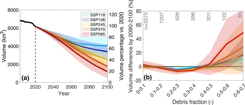
L. Compagno et al.: Regional-scale modelling of supraglacial debris 1705
(step 2) but by keeping unaltered the model parameters de-
termined in step 1 (and potentially step 3). This strategy thus
preserves the glacier-specific climate conditions (precipita-
tion totals and temperature) but adjusts the glaciers’ temper-
ature sensitivity for snow and ice melt in order to reproduce
the observed mass change even without directly accounting
for the melt-reduction process of supraglacial debris cover-
age.
4.2 Debris-cover evolution
4.2.1 Calibrating lateral debris expansion
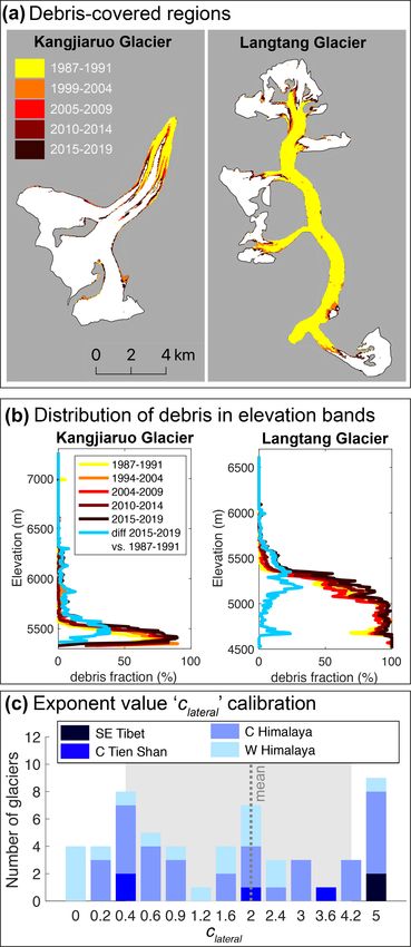
To determine clateral , we use the debris-cover observations
obtained from the Landsat scenes (set S1, composed of
55 glaciers with debris; see Sect. 2 and e.g. Fig. 5a). First,
the evolution of the debris’ lateral expansion is calculated
for each glacier and each elevation band (e.g. Fig. 5b). Then,
calibration is performed by comparing the lateral expansion
of debris as observed and as modelled using different clateral
factors (ranging from 0 to 5). More specifically, we take the
debris extent detected on each Landsat scene as the initial
condition, and we simulate each glacier independently for
each clateral . Finally, we calculate the root-mean-square er-
ror (RMSE) between modelled and observed lateral debris
expansion over the period captured by our data set and for
each of the 55 glaciers. For each glacier, we select the clateral
which results in the lowest RMSE (see Fig. 5c). The mean
of the selected clateral is clateral = 2.0, while the 0.25 and
0.75 quantiles are clateral = 0.4 and clateral = 4.2, respectively.
The mean value is used for all further modelling; i.e. the
same value is applied for all glaciers in HMA, whilst the re-
sult’s sensitivity to the uncertainty in clateral is analysed in
Sect. 5.2.1.
4.2.2 Calibrating debris thickness evolution
To determine cthickening , a three-step procedure is used. In
a first step, we map where debris cover appeared for the
first time between ∼ 1974 (Hexagon satellite imagery) and
∼ 1989 (oldest Landsat satellite image). This is done for
12 glaciers with Hexagon satellite observations in set S1
(out of the total of 18 glaciers in set S1) within three sub-
regions (Central Himalaya, East Himalaya, and West Tien
Shan). The six remaining glaciers are not used because a
clear signal of debris formation is lacking between ∼ 1974
Figure 5. (a) Evolution of the debris-covered area of Kangjiaruo
and ∼ 1989. In a second step, we extract the debris thickness
Glacier and Langtang Glacier as inferred from five Landsat scenes.
at the locations used in the debris thickness data set of Mc- (b) Same as (a) but divided into 10 m elevation bands. The blue line
Carthy et al. (2021). Recall that the latter data set represents shows the lateral expansion of the debris cover as observed between
the debris condition for 2000–2016. Combined, this informa- the oldest (1987–1991) and the newest (2015–2019) Landsat scene.
tion provides us with an estimate for the mean debris thick- (c) Distribution of clateral resulting in the lowest misfit between ob-
ening rate between ∼ 1981 (mean between 1974 and 1989) served and modelled debris-fraction evolution (given per number
and ∼ 2008 (mean between 2000 and 2016). In a third step, of glaciers). The grey dashed line shows the mean value, while the
we compute the difference between observed and modelled grey rectangle shows values within the 0.25 and 0.75 quartiles.
debris-thickening rate for each glacier. To do so, the 12 se-
https://doi.org/10.5194/tc-16-1697-2022 The Cryosphere, 16, 1697–1718, 2022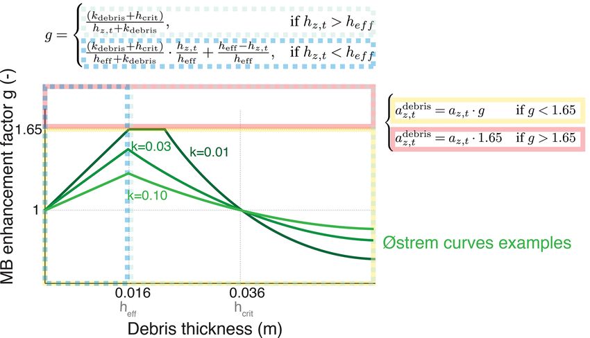
1706                                                      L. Compagno et al.: Regional-scale modelling of supraglacial debris

Figure 6. Difference between observed and modelled debris thickness for the period ∼ 1981–2008 (circles) using different thickness tuning
factor (cthickening ) values. Glaciers IDs refer to RGI 6.0 (RGI Consortium, 2017).

lected glaciers are modelled with cthickening values ranging           5     Model evaluation
between 0 and 2 (Fig. 6), and the value minimizing the differ-
ence to observations is chosen. We find cthickening = 1.0. This        5.1    Mass balance
value and the result’s sensitivity are evaluated in Sect. 5.2.2.
                                                                       To evaluate the performance of the mass-balance module,
4.3    Ice flow                                                        we compare the modelled mass balances for 21 glaciers
                                                                       in HMA against observations provided by the World
The ice-flow module is initialized and calibrated by generat-          Glacier Monitoring Service (WGMS, 2020). For glacier-
ing a glacier-specific steady state for a specified point in time      wide annual mass balance, the bias (measured–modelled)
in the past. The exact timing of this point in time depends on         is −0.24 m w.e. a−1 , and the RMSE is 0.55 m w.e. a−1 (see
both climate and glacier response time (see Compagno et al.,           Fig. S2). Observations aggregated to elevation bands show a
2021, for more details). Starting from this steady state (on           bias of −0.38 m w.e. a−1 and a RMSE of 0.77 m w.e. a−1 . For
average between 1979–1983 and 1990–1996 in this study),                glacier-wide winter balance, the bias is 0.23 m w.e. a−1 , and
the glacier is transiently modelled up to the glacier inven-           the RMSE is 0.41 m w.e. a−1 (see Fig. S3). These results are
tory date by using ERA5 reanalysis data. To ensure that the            satisfactory in comparison to other regional-scale modelling
so-modelled glacier volume and length are consistent with              studies (e.g. Marzeion et al., 2012; Huss and Hock, 2015;
the available observations, the procedure is repeated by itera-        Radić and Hock, 2014).
tively changing two parameters: the deformation-sliding fac-
tor and a mass-balance bias applied during the generation of           5.2    Debris evolution
the steady state (see Zekollari et al., 2019, for more details).
Since the entire procedure is performed before the glacier-            In this section, the three parameterizations included in our
specific inventory year, debris cover is considered to be static       debris-evolution module (see Fig. 4) are evaluated against in-
(as given by the observations). Once calibrated, the model is          dependent data sets.
forced by ERA5 reanalysis data (until 2020) and GCM out-
put data to simulate the future glacier evolution (2020 until
2100).

The Cryosphere, 16, 1697–1718, 2022                                                        https://doi.org/10.5194/tc-16-1697-2022
L. Compagno et al.: Regional-scale modelling of supraglacial debris 1707
Figure 7. (a) Histograms of the misfit between observed and modelled lateral debris expansion when using clateral = 2 (grey) and when
deactivating the module (clateral = 0, orange; no evo: without evolution). (b) Same as (a) but divided into glaciers and distinguishing between
different reference years (corresponding to the Landsat scenes). The colour of each circle represents the misfit (%). (c, d) Modelled debris-
area evolution (red–white–blue shades) and debris-area evolution as observed in the Landsat scenes (black dashed line) for four selected
glaciers (indicated by arrows).
5.2.1 Evaluating lateral expansion of debris ∼ 1974. In this case, the mean misfit between observed and
modelled debris fraction is 4.4 % (Fig. 7a, orange histogram),
i.e. substantially higher than for the case in which the debris
To evaluate the parametrization for lateral debris expan-
area evolution is included. The experiment thus shows the
sion, 18 glaciers (set S1 with Hexagon satellite observations)
importance of accounting for debris expansion when mod-
within three subregions (Central Himalaya, West Himalaya,
elling long-term glacier evolution.
and West Tien Shan) are simulated from 1974 to 2020 (forc-
ing the model with ERA5 climate). The model is initialized
with debris extents extracted from Hexagon satellite images 5.2.2 Evaluating debris up-glacier expansion
of ∼ 1974 (see Sect. 2). The modelled debris-area evolution
is evaluated between 1989 and 2017 against the time series of To evaluate the parametrization for the up-glacier debris
debris extents obtained from Landsat (three to five observa- expansion, we use the same experiment setup as above
tions per glacier). We calculate the misfit between modelled (Sect. 5.2.1). We initialize the model in 1974 and force it un-
and observed debris-cover fraction for each elevation band. til 2020 but now focus on the transition zone between debris-
Note that this is the same procedure as used for calibration covered and bare-ice surfaces. For each glacier with observed
(see Sect. 4.2), with the difference that for model initializa- debris extents from Hexagon and Landsat (of set S1), we
tion we use debris extents from Hexagon imagery rather than extract from the Landsat scenes the highest elevation bands
Landsat (Fig. 7). The mean misfit of debris fraction obtained that have a debris-covered fraction of ≥ 10 %, 20 %, 30 %,
by this procedure is 0.7 % (Fig. 7a, grey histogram), with 42 40 %, and 50 %. We perform the same extraction procedure
of the 78 evaluations indicating a misfit < ±2 % (Fig. 7a, b). for the modelling results. Then we compute for each glacier
A good model performance is also shown by analysing the and each Landsat scene the elevation misfit between obser-
glacier-specific lateral expansion of debris (Fig. 7c, d). vations and modelling results (Fig. 8). The mean misfit is of
The performance of our parametrization for lateral debris +27 m.
expansion can also be evaluated by disabling this process in Again, an alternative way for evaluating our approach is to
the model. We do so by initializing the model as above but turn off the up-glacier expansion parametrization, thus pre-
by prescribing a constant debris cover, taken to be the one of scribing a temporally constant debris cover, set to be the
https://doi.org/10.5194/tc-16-1697-2022 The Cryosphere, 16, 1697–1718, 20221708 L. Compagno et al.: Regional-scale modelling of supraglacial debris
indicate high glacier-to-glacier variance of cthickening but also
show that the proposed parametrization is rather insensi-
tive to the weakly constrained value of cthickening (see also
Sect. 7).
6 Results
6.1 Glacier-specific simulations
In order to illustrate the detailed model results at the scale
of an individual glacier, we focus on the well-investigated
Langtang Glacier (Central Himalaya). A similar illustra-
tion for Baltoro Glacier (Karakoram) and Inylchek Glacier
(West Tien Shan), which showed patterns similar to Lang-
tang Glacier, is given in Figs. S5 and S6, respectively.
Figure 9a shows a profile view of the glacier and debris-
cover evolution of Langtang Glacier according to our model
results and SSP245. Under this scenario, Langtang Glacier
would lose 43 % of its 2020 ice volume by 2050, despite the
terminus retreating by less than 300 m (i.e. only 2 % of its
2020 length). The limited retreat can be attributed to the 0.5–
1 m thick insulating debris cover present on the entire glacier
tongue, which reduces Langtang Glaciers’s ice melt by a fac-
tor of about 3 compared to the hypothetical situation with no
debris. The approximately linear dependence between sur-
face mass balance and elevation, which is typical of clean-
ice glaciers, is suppressed for Langtang Glacier, since debris
cover is thicker at lower elevations than it is for higher ones
Figure 8. Misfit between observed and modelled highest elevation
with a lateral debris expansion ≥ 10 %, 20 %, 30 %, 40 %, and 50 %. (Bisset et al., 2020; Miles et al., 2021). This leads to a nearly
The debris-cover evolution module is activated in panel (a) and de- homogeneous downwasting of the ablation zone (e.g. Pel-
activated in panel (b). licciotti et al., 2015; Ragettli et al., 2016) rather than to a
retreat of the terminus (e.g. Benn et al., 2012). This causal-
ity is confirmed when the evolution of Langtang Glacier is
one inferred for ∼ 1974. For this case without up-glacier de- re-computed using the same climatic conditions but when
bris expansion, we re-compute the misfit between observed re-calibrating the model parameters to match the observed
and modelled elevation with a debris fraction ≥ 10 %, 20 %, volume changes without activating the debris-cover module
30 %, 40 %, and 50 %. This results in a misfit of +55 m, (Fig. 9b). In this case, the glacier would lose 45 % of its 2020
i.e. almost 2 times larger compared to when the up-glacier ice volume by 2050 (i.e. very similar to explicit debris mod-
debris expansion parametrization is activated, indicating the elling) but would retreat by about 2700 m (i.e. 20 % of its
importance of taking up-glacier debris expansion into ac- 2020 length). The latter is 10 times more than when includ-
count as well. ing the effect of supraglacial debris.
Figure 9a and c show a spatial representation of the debris-
5.2.3 Evaluating debris thickness evolution cover evolution according to the three implemented param-
eterizations. At 5500 m a.s.l. for instance, the fraction of de-
To evaluate the debris thickness evolution parametrization, bris increased by 87 % between 2025 and 2100. This result is
we compare model results against the evaluation data set S2, driven by the projected lateral debris expansion. As a result
i.e. 11 glaciers distributed in four regions (East Himalaya, of the projected up-glacier migration, instead, the maximum
Karakoram, West Tien Shan, and Inner Tibet). By setting elevation with supraglacial debris would increase by 280 m
cthickening = 1.0, the mean misfit between observed and mod- for the same time period. Finally, the local debris thickness
elled debris-thickening rate is 0.07 m. For cthickening = 0.0 at 5500 m a.s.l. is projected to increase by 0.23 m over the
(i.e. no debris thickness evolution), it is 0.17 m (see Fig. S4). period 2025–2100.
The model, thus, performs better when the debris thickness The presence of supraglacial debris alters glacier mass
evolution parametrization is activated. Taken together, this balance, hence influencing the debris-cover evolution itself.
evaluation and the calibration results (Sect. 4.2.2) not only With higher mass loss, our model results show that both
The Cryosphere, 16, 1697–1718, 2022 https://doi.org/10.5194/tc-16-1697-2022L. Compagno et al.: Regional-scale modelling of supraglacial debris 1709 Figure 9. (a) Modelled evolution of Langtang Glacier when debris is explicitly accounted for. The results refer to SSP245. Note that the debris thickness (grey) is exaggerated by a factor of 500 for visibility. The three parameterizations included in the debris-cover module (cf. Sect. 3.2 and Fig. 4) are indicated by the circled, coloured numbers and described in the text. (b) Same as (a) but accounting for debris implicitly; i.e. glacier evolution is not modelled with the new debris-cover module but by re-calibrating some of the model parameters to match observed long-term mass balance (see Sect. 4.1 for details). (c) Model results extrapolated to 2D (see Supplement for the method used for extrapolating from one to two dimensions, and note that the extrapolation is for visualization purposes only; i.e. it does not affect the presented results). For every SSP, the evolution of (d) debris-cover fraction, (e) glacier volume with explicit debris-cover modelling, (g) debris thickness, and (h) glacier area with explicit modelling is shown. (f, i) For every SSP the difference in glacier volume and area obtained when explicitly and implicitly modelling the debris cover. The shaded ranges represent 1 standard deviation of all climate model members included in a given SSP. debris-covered area and debris thickness increase, thus re- simulations show that the fraction of debris-covered area ducing ice melt. Nevertheless, higher mass loss also leads to is expected to increase until 2060, reaching a maximum of glacier retreat and downwasting of the debris-covered glacier 55±2 % (mean and standard deviation of all model members tongue, thus reducing debris-cover extent due to glacier area considering SSP245) relative to the remaining glacier area. loss. Therefore, a competition between debris increase and After reaching this debris peak fraction, a fast decline is mod- reduction arises after 2060. For Langtang Glacier, model elled due to disintegration of the debris-covered tongue. De- https://doi.org/10.5194/tc-16-1697-2022 The Cryosphere, 16, 1697–1718, 2022
1710                                                       L. Compagno et al.: Regional-scale modelling of supraglacial debris

Figure 10. Evolution of (a) debris-covered fraction and (b) debris thickness for all HMA glaciers and as an average for the respective SSP.
The shaded bands represent 1 standard deviation of all climate model members. The grey line indicates the case in which the debris-evolution
module is disabled and only today’s debris cover is used in the modelling.

pending on the emission scenario, the debris-covered fraction           volume loss only differing by between 1 % and 6 %, depend-
reaches between 28 ± 6 % (SSP119) and 18 ± 5 % (SSP585)                 ing on the SSP (Fig. 9h, i). This indicates that constraining
by 2100 (Fig. 9f). Note that the fraction refers to the evolving        the model to past glacier mass loss yields similar results, even
glacier geometry and not to the geometry at inventory date.             when considering Langtang Glacier to be a clean-ice glacier.
By turning off the debris-evolution parametrization (expan-             In that case, however, surface mass-balance gradients would
sion and thickening) and by using presently observed debris             not consider the effect of debris cover (see e.g. Fig. S7),
extent and thickness instead (grey line in Fig. 9f), the de-            with consequences for the geometry evolution, runoff, and
bris fraction would continuously decrease, reaching between             surface-elevation feedbacks.
14 ± 7 % (SSP119) and 1 ± 1 % in 2100 (SSP585).
   Compared to 2020, the modelled mean debris thickness                 6.2    Regional glacier evolution
of Langtang Glacier is expected to increase by 35 ± 5 % and
reach its maximum in 2065 (SSP245). The variation between               The area-averaged debris-cover fraction of all glaciers in
individual SSPs is relatively small. Different SSPs give rise           HMA is expected to be between 14 % and 24 % by 2100
to different thickness evolution trajectories however, reach-           compared to the 12 %–13 % observed today (Fig. 10a; note
ing between −7 ± 10 % (SSP119) and −75 ± 19 % (SSP585)                  that these numbers refer to glaciers with an area > 2 km2
of the 2020 debris thickness by 2100. This counter-intuitive            and that the debris-cover fractions are computed for the tran-
decrease in average debris thickness can be explained by the            siently evolving glacier areas). Generally, the debris-cover
evolution of both debris extent as well as glacier geometry.            fraction is projected to be higher for higher-emission sce-
Indeed, the expansion of thin debris to higher areas and the            narios (i.e. scenarios implying a higher air temperature in-
loss of presently thick debris on the downwasting tongue re-            crease). The expected increase in debris-cover fraction is
sults in a mean debris thickness decrease (see also Sect. 7).           due to both lateral and up-glacier expansion. Without ac-
When neglecting the evolution of debris extent and thickness            counting for debris-cover evolution, the debris-cover frac-
(i.e. the change in debris thickness is only due to glacier ge-         tion, however, is projected to be between 8 ± 1 % (SSP119)
ometry change), the mean debris thickness would decrease                and 6 ± 1 % (SSP585). This highlights the importance of
by between 30 ± 18 % (SSP119) and 80 ± 35 % (SSP585)                    accounting for dynamic debris-cover evolution in process-
by 2100. Together with the debris-fraction evolution, this              based studies. Our results also show that under low-emission
demonstrates that it is relevant to account for transient debris-       scenarios, the competing processes of debris expansion and
cover changes in process-based models, at least for low- to             glacier retreat tend to reach an equilibrium at the end of the
medium-emission scenarios (Fig. 9d).                                    century. For high-emission scenarios, instead, debris-cover
   By 2100 and when explicitly modelling debris-cover                   expansion dominates over glacier retreat.
changes, Langtang Glacier is projected to lose between 69 ±                Between 2020 and 2100, the area-averaged debris-cover
14 % (SSP119) and 98±2 % (SSP585) of its 2020 ice volume                thickness of all glaciers in HMA (again, with area > 2 km2
(Fig. 9e). If debris cover is implicitly taken into account, very       and not of surge type) is expected to slightly increase by
similar results are obtained, with simulated 2100 area and              about 5 % or 2 cm compared to today; see Fig. 10b. Inter-
                                                                        estingly, a very similar change is found for both low- and

The Cryosphere, 16, 1697–1718, 2022                                                          https://doi.org/10.5194/tc-16-1697-2022
You can also read