MOVIE SUCCESS PREDICTION AND PERFORMANCE COMPARISON USING VARIOUS STATISTICAL APPROACHES
←
→
Page content transcription
If your browser does not render page correctly, please read the page content below
International Journal of Artificial Intelligence and Applications (IJAIA), Vol.13, No.1, January 2022

                 MOVIE SUCCESS PREDICTION AND
                PERFORMANCE COMPARISON USING
                VARIOUS STATISTICAL APPROACHES
         Manav Agarwal, Shreya Venugopal, Rishab Kashyap and R Bharathi

                     Department of CSE, PES University, Bangalore, India

ABSTRACT
Movies are among the most prominent contributors to the global entertainment industry today, and they
are among the biggest revenue-generating industries from a commercial standpoint. It's vital to divide
films into two categories: successful and unsuccessful. To categorize the movies in this research, a variety
of models were utilized, including regression models such as Simple Linear, Multiple Linear, and Logistic
Regression, clustering techniques such as SVM and K-Means, Time Series Analysis, and an Artificial
Neural Network. The models stated above were compared on a variety of factors, including their accuracy
on the training and validation datasets as well as the testing dataset, the availability of new movie
characteristics, and a variety of other statistical metrics. During the course of this study, it was discovered
that certain characteristics have a greater impact on the likelihood of a film's success than others. For
example, the existence of the genre action may have a significant impact on the forecasts, although another
genre, such as sport, may not. The testing dataset for the models and classifiers has been taken from the
IMDb website for the year 2020. The Artificial Neural Network, with an accuracy of 86 percent, is the best
performing model of all the models discussed.

KEYWORDS
Regression Models, Clustering Techniques, Time Series Model, Artificial Neural Network, Movie Success,
Statistical Significance.

1. INTRODUCTION
Movies are one of the most important contributing factors to the entertainment industry in the
world today, and from a commercial perspective are among the highest revenue-generating
businesses [1]. Hence from a movie industry point of view, it is important to know whether a
movie that they are thinking of making will be successful. There are plenty of factors such as the
genre of a movie, the popularity of a movie based on its votes, critical judgement, and so on
which influence the choices made by people to watch certain movies of their liking. Thus, to
identify a movie that is worth watching, people look into various websites and articles such as
Metacritic, Rotten Tomatoes, IMDb and many more sites that give us the rating of the movie.
Thus, the analysis involves the study of these user ratings and the other factors that affect the
movie and this helps us identify whether a movie is truly successful or not. This would help those
who are creating movies make better movies and thus get more revenue. It will also make sure
that the audience gets to watch movies that they enjoy. We wish to exploit the various techniques
and tools used to uncover useful information from a variety of data that provides information
about movies to infer various useful traits in it using which we would like to build a movie
success predictor. The data is used in predictive models which include regressors, classifiers and
time series models. Each of these models uses the attributes associated with the movies as
independent values used to predict the outcome rating of the movie. Crossing a certain pre-set

DOI: 10.5121/ijaia.2022.13102                                                                               19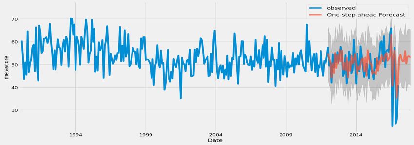
International Journal of Artificial Intelligence and Applications (IJAIA), Vol.13, No.1, January 2022
threshold classifies it as a success, else we deem the movie unsuccessful. The models that we use
consist of regression models such as Linear Regression, Logistic Regression, Ridge and LASSO
Regression. Classifiers include machine learning models such as K-Means and Support Vector
Machine. An Artificial Neural Network is also used. The final model that we use is Time Series
analysis which allows us to observe the variations that take place over the years on the movie
ratings and to identify trends and seasonality in the data if it exists. Hence the main contributions
of this work are:

    1. Find the kind of model that predicts the success of a movie the best.
    2. Perform a comparative study between various models and also look into the statistical
       significance of each model.
    3. Understand what features influence the success or failure of a movie.
    4. Test it against the data of 2020, the data available for movies that are being released
       recently.
    5. Determine if the attributes for the model are easily available.

2. LITERATURE SURVEY
Before the literature survey, we had to analyze and select the right dataset to be used for this
purpose through which we concluded on using the IMDb Extensive dataset [2]. This is
accompanied by movies and their attributes scraped from the IMDb website for those released in
the year 2020 through data mining techniques [3-4]. As shown by Abidi et. al [1] the next set of
steps would be to identify the list of attributes that assist in predicting how popular a movie is
through a thorough investigation into all the properties of a given movie. . They mention that
movie genres contribute a vital role in the popularity of the movie because the movie industry
firmly makes decisions on what type of movie customers of different ethnic groups liked, rate,
and favoured the movie. Thus, to study such attributes and use them for prediction, we utilize a
wide range of regression models [5] and Machine Learning techniques [6-7] to carry out our
predictions, including the use of Neural Networks [8] for more efficient classification. To add
value to our experiments, we perform a comparative study similar to that done by Dhir and Raj
[9] who have compared specifically for machine learning models. Before that, we check the
credibility of a model by performing various statistical tests [12-13] whose comprehensive
explanation is the highlight of our paper. The best performing model in this paper gives an
accuracy of 86% which holds good in comparison to the works done by Sharma et al [14] and the
models used by Dhir and Raj [9].

3. PROPOSED METHODOLOGY
From the literature survey, we have gathered information about the various technologies and
methods used to predict how successful a movie is. With reference to them, we build on some of
the important models used and prove how significant they are by applying various statistical tests
on them. Figure 1 shows the phases of our experiment along with the models we are testing. Data
is first collected from various sources that can be either from pre-existing datasets that are curated
by someone else or by scraping it directly from the internet. Through studying the statistical
significance of the models we aim to prove the validity and merit of each type of model. In doing
so we deduce the best model that can be used to predict the success rate of a given movie with the
best performance. In the entire process, we use python programming language for our analysis as
the libraries provided for statistical analysis allows for a much smoother and efficient process.

                                                                                                           20
International Journal of Artificial Intelligence and Applications (IJAIA), Vol.13, No.1, January 2022

                                     Figure 1. Proposed Methodology

As can be seen in Figure 1 the entire project is divided into 4 phases namely Data Collection, Pre-
Processing, Building the prediction models and the testing phase. In the Data collection phase we
collected data from two sources, a pre-existing Extensive IMDb dataset from Kaggle which was
used as the training and the validation dataset for the models and the other part of the dataset was
obtained by scraping data off of the IMDb website which formed the testing dataset for these
models. This is to ensure that whatever models that were made work well in a realistic scenario
with the attributes that are available in the present day and will continue to work properly in the
future. In the next phase, which is the Pre-Processing phase, we clean the data from both the
sources and convert them to a form that can be used to develop and train the models. The next
phase involves building various models using the dataset that has been created and testing them
on the scraped dataset. In the next phase, we put the models that have been built through the
testing dataset and perform statistical tests on them to check their validity.

4. DATASET DESCRIPTION
As mentioned above, this project uses the IMDb dataset [2]. This dataset consisted of 4 files -
movie related data such as budget, duration and so on, the data that give the number of votes or
ratings for each movie for multiple demographics, data that involves biographical details of those
that are involved in the movie-making industry like their place of birth, spouse etc and finally
another file to act as a mapping between these files. Not all of the attributes present in the dataset
were taken into consideration for the analysis. Some of them were filtered out based on the
relevance of the problem at hand. For example, attributes related to the personal lives of the
people involved in the film industry were not required for predicting whether a movie would be
successful. Attributes such as the personalities in the movie were not used since they are
categorical and we wanted to restrict this analysis to remain as numeric as possible. Some of the
major attributes that were a part of the data include the movie rating itself, followed by the genre,
top voter ratings, total votes, duration of the movie and the release date. Here, the genre is the
only categorical variable that was used in the analysis since the number types of the genre is 21
which is less compared to the number of actors or directors or other personalities. A total of
81274 movies have been obtained from the dataset, and the values are first cleaned in the
preprocessing stage before it is split into training and testing datasets. The split is done with
respect to the year of release of a given movie. Web scraping has also been used to extract data
from the IMDb official website, from which we obtain all the movies released in the year 2020,
which is combined with the previous testing dataset to create the final validation dataset.

                                                                                                           21
International Journal of Artificial Intelligence and Applications (IJAIA), Vol.13, No.1, January 2022
5. PRE-PROCESSING
The first step of pre processing is to remove all null values and outliers through the process of
elimination, or replacement by mean or median values if necessary. The attribute “budget” had
values in different kinds of currencies, which would have caused problems if they were used as-
is. Hence, for this analysis, the movies that are considered are only in US Dollars. One of the
most important pre processing techniques used is the Multi Label Binarizer [15] which allows us
to encode attributes having more than one feature such as the genre. To do this, we list out all the
sub-features of the genre attribute as columns and for each movie, we put 1 if the movie belongs
to that genre, else we leave it as 0 by default. This process is repeated for all movies until we
have a list of numeric values depicting the genres that belong to the movie and those that do not.
This way the genre which previously represented a one to many relationship mapping with the
help of one attribute gets converted into a better representation with discrete form, making it easy
for classification. Movies that range from the years 1990 to 2015 are grouped together to create
the training dataset, and movies from 2015 to 2020 are considered as our testing dataset. Movies
older than 1990, were too old to use in a model for predicting movies that are made today
because there was a lot of difference in the social environment. Besides, the data for older movies
was very scarce, incomplete compared to the data entries for newer movies. To implement our
classification, we have chosen the “metascore” value from the dataset to act as our dependent
variable for our research. This attribute represents the overall numeric rating of any given movie
between 0 to 100, 0 being the worst possible score and 100 being the best possible score that a
movie can receive. To make the classification easier, we group the metascore values into three
types of clusters known as “bins” [16], where each bin represents a flop, a mediocre and a
successful movie. Movies that have a metascore from 0 to 33 are considered to be a flop, those
that have a metascore from 33 to 66 mediocre and those that have a metascore that is between 66
and 100 is considered as a hit. All the models used are tuned to output the predicted metascore
values based on the categories created here.
6. FEATURE SELECTION
Once the data is pre-processed, feature selection is performed to determine which attributes from
our pre-processed dataset can go into the respective model. This process to a great extent depends
on trial-and-error, that is, taking a random subset of features and seeing how the model performs
and if that performance is better or worse than another group of attributes. However, there are
some formal ways of tackling this too, some of which have been employed in this analysis. The
first is using the values that were obtained by performing a correlation analysis for the numeric
attributes in the dataset to make a decision on which set of attributes best work together. For each
pair of numerical attributes, Pearson correlation is used. When selecting features for a model it is
important that those features must have a good correlation with the dependent variable which is
the “metascore” and also, those features that are being used as independent variables for a model
should not be correlated with one another. This situation leads to multi-collinearity. Next comes
the use of the Variance Inflation Factor (VIF) which for a given set of attributes shows if they can
be used together in a model. The subset of attributes that must go into the VIF analysis is
determined by trial and error. All the models in this work except for those that use regularization
techniques such as Ridge and Lasso regression used the correlation analysis and VIF for its
feature selection process.
22International Journal of Artificial Intelligence and Applications (IJAIA), Vol.13, No.1, January 2022
7. REGRESSION METHODS
Regression is a technique that uses the Ordinary Least Squares method to predict certain values
given certain inputs. The outputs of regression models with the exception of Logistic Regression
are usually continuous estimates of the dependent variable. They are not used for classification.
But since the problem that we are looking into involves the classification of a movie into
Successful, Unsuccessful and Mediocre, the values predicted from the regression models need to
be binned into the 3 categories before testing for accuracy.
7.1. Simple Linear Regression
The first type of model we look into would be the Linear Regression model using a single
variable. Simple Linear Regression (SLR) is a statistical model in which there is only one
independent variable and the functional relationship between the dependent variable and the
regression coefficient is linear[12]. The regression line is of the form:
Here, the dependent variable Yi is known as the outcome or response variable, and Xi Is known
as the independent variable for the ith term, and the beta coefficients are known as the regression
parameters. The final value-added is known as the random error value or the residual that is
obtained on performing the regression. In our case, we use the metascore as our dependent
variable. We make use of the Variance Inflation Factor or VIF to calculate the multicollinearity
among all the attributes present. Only one attribute has to be selected since SLR involves only a
single independent variable, and hence we choose the attribute having the highest VIF value.
From the list of features, we choose the top1000_voters_rating having the highest VIF value as
our independent variable. The SLR model is trained using this attribute for all movies. As seen
from Figure 2, budget has the lowest VIF value of 0, while top1000_voters_ratings is the highest
with a value of 0.55.
Figure 2. VIF distribution for the list of features
Once we have our trained model, we use the testing dataset to predict the future values, and then
make a comparison between the true and predicted values. The accuracy of the model is
calculated using a confusion matrix, which checks whether the values have truly been classified
based on their values or falsely classified. Tests for statistical significance are performed on the
model on completion of training. . On completing the proof of statistical significance, we move
on to testing the model with the 2020 dataset, which yields an accuracy of 0.5833. The only
difference in this is the fact that we take the avg_vote value in-place of the
top1000_voters_rating.
23International Journal of Artificial Intelligence and Applications (IJAIA), Vol.13, No.1, January 2022
Figure 3. SLR model
7.2. Multiple Linear Regression
In a Multiple Linear Regression (MLR) model, there are many independent variables as opposed
to the single independent variable in the SLR to estimate the target variable which is the
metascore in this case. For this model, there are a total of sixteen attributes including the
“top1000_voters_rating” along with twelve attributes that are the dummy variables generated by
the Multi Label Binarizer for the genre. The VIF test again determines which features to select,
and OLS tests, as well as the hypothesis tests like the Jarque Bera test and Lagrange’s Multiplier
test, are performed to check for statistical significance. This model has an accuracy of 0.7116.
Figure 4 shows a three-dimensional view of the MLR model using a sample of two of the
independent variables along with the metascore. For the 2020 dataset, the same model is used
giving an accuracy of 0.608.
Figure 4. MLR model
7.3. Logistic Regression
Logistic Regression is a non-linear regression technique that is used when a set of independent
variables are used to make a binary classification[13]. The main aim is to find the conditional
probability of the occurrence of the event which facilitates the classification. Here, there is a
slight change from the original steps that were performed for the target variables where now the
metascore will be binned into two categories which are successful and unsuccessful instead of
24International Journal of Artificial Intelligence and Applications (IJAIA), Vol.13, No.1, January 2022
three. The model gives an accuracy of 0.76. The ROC-AUC curve plotted from the confusion
matrix of the results is shown in Figure 5. A Wald’s test is performed to check the statistical
significance of each of the independent variables used. This is similar to performing a t-test in the
MLR model [12]. Pseudo R2 values are used to compare the intercept-only model to the model
with the independent variables as it is not possible to calculate R 2 directly. The analysis of the
2020 dataset for Logistic Regression gives an accuracy of 0.6833.
Figure 5. Plot to show the ROC-AUC curve
7.4. Regularization Techniques
Regularization in a regression model is a technique that prevents overfitting in the model by
penalizing the coefficients involved in the regression equation. Ridge regression is a model that
falls under the category of regularization techniques. It follows the L2 regularization method that
reduces the summation of squared values of coefficients to the regression equation as penalties,
which helps to penalize the multi collinearity [12]. The regularization parameter is set at 1150 for
Ridge Regression, and the model gave us an accuracy of 0.74 analysing. LASSO regression on
the other hand is a regularization technique that follows the L1 norm. This means that it adds the
absolute value of coefficients as penalties to the cost function. We perform the same procedure as
we did in the case of Ridge regression, where the regularization parameter is set to 0.145, and we
obtain an accuracy of 0.72 for this model. To test both the models, we once again use the 2020
testing dataset to confirm our results, obtaining an accuracy of 0.6, and we further perform
statistical tests to prove their significance as displayed in the Results section.
Figure 6. Residual plots for Ridge regression (left) and LASSO regression (right)
25International Journal of Artificial Intelligence and Applications (IJAIA), Vol.13, No.1, January 2022
8. CLASSIFICATION METHODS
Unlike the regression models, the classification model outputs don’t require binning before
analysis for accuracy. Here a supervised classifier (SVM) and an unsupervised clustering
technique (K-Means) is used for solving the movie success prediction problem.
8.1. K-Means Classifier
K-Means clustering is a non-hierarchical clustering method in which the number of clusters (K)
is decided a priori, in other words, decided prior to the execution of the model [12]. In our study
for this paper, it has been used as a classifier where each cluster is considered as a separate class.
In this case, we change the value of K to 3 to represent each of the metascore bins mentioned
earlier [12]. On plotting the model, we obtain a final accuracy of 0.5. To prove the statistical
significance, we perform the silhouette test, which is a technique used to evaluate the quality of
the clusters created by the K-Means method, which calculates how similar each cluster is by size
by checking the intra-cluster point distance and inter-cluster distances. The plot shown in Figure
7 shows the clusters created on testing the model using the 2020 dataset, from which we obtain
an accuracy of 0.42.
Figure 7. Centroid positions for KMeans Clustering
8.2. Support Vector Machine
The Support Vector Machine or SVM is a very powerful clustering technique that uses
hyperplanes to distinguish between clusters. Traditionally, we use a single hyperplane to do this,
but in our case we have made use of two hyperplanes to divide the outcome into three clusters,
each corresponding to the three categories made to the metascore values. This model results in an
accuracy of 0.71 using the training dataset, which is then used against the 2020 testing dataset to
obtain an accuracy of 0.62. As a proof of statistical significance, a silhouette test is performed to
check whether the model’s clusters are of good quality as we had done earlier for the K-Means
classifier.
Figure 8. Plot to depict the cluster formation in SVM
26International Journal of Artificial Intelligence and Applications (IJAIA), Vol.13, No.1, January 2022
9. TIME SERIES ANALYSIS
Forecasting is a process that uses past and present values to predict the values for the future. This
is done by analysing and obtaining patterns from the data such as trend, seasonality and so on.
These serve as the parameters of the model and help in defining what kind of model needs to be
used for the time series analysis. For this problem statement, the date on which the film is
released is taken as the primary variable that is being under analysis. On plotting the metascore
value against the date_published attribute to get the time-series graph for the entire dataset and
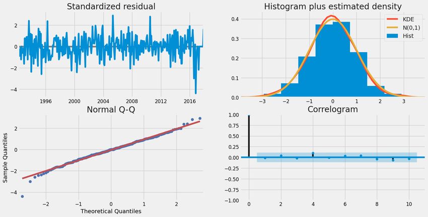
conducting some statistical tests we obtain Figure 9 and Figure 10.
Figure 9. Various plots for statistical significance of time series model
Figure 10. Forecasted value compared to actual value residual plot
These statistical tests to determine its patterns and characteristics as mentioned above include the
Augmented Dickey-Fuller Test for stationarity and analysis of the ACF and PACF plots for the
autocorrelation and moving average parameters. From the results obtained from these tests along
with a comparison of the AIC values the time series model to be used is finalized as the Seasonal
Auto-Regressive Integrated Moving Average with eXogenous factors model, or in short, the
27International Journal of Artificial Intelligence and Applications (IJAIA), Vol.13, No.1, January 2022
SARIMAX model. We can see that the model gives us a roughly accurate result for the forecast.
We plot the same for our 2020 dataset, using the SARIMAX model we used before to get similar
outputs as in Figure 11.
Figure 11. Observed vs forecasted values
10. ARTIFICIAL NEURAL NETWORK
The Artificial Neural Network is the most complex model used for prediction, and here, we make
use of the Multi-Layer Perceptron network for our classification. The training data is fed into the
model and run over multiple epochs. .The model gives us an accuracy of 86.16% and on plotting
the loss curve, we notice a gradual decline in the loss percentage, which indicates a rapid
improvement in performance after every epoch. Steps to reduce overfitting have also been taken.
These include limiting the maximum number of iterations and implementing Early Stopping. The
loss curve for the model is displayed in Figure 12. On testing the model with our validation 2020
dataset, we obtain a final accuracy of 88.056%.
Figure 12. Loss Curve for the ANN
28International Journal of Artificial Intelligence and Applications (IJAIA), Vol.13, No.1, January 2022
11. RESULTS AND INTERPRETATION OF VALUES
11.1. Regression
Wald’s test for Logistic Regression proved the statistical significance of the model in Table 1.
Wald’s test is used to check if each of the variables involved in Logistic Regression will give
statistically significant results, indicated by the p-values depicted below. The Chi-square tests,
though high in number for a couple of attributes, on the whole, proves that the Logistic regression
model is still significantly valid in terms of the results we obtain from it.
Table 1. Wald’s Test for Logistic Regression
X Chi^2 p-value > Chi^2
const 1062.614071 4.411953e-233
top1000_voters_rating 1104.475166 3.517505e-242
Action 53.033523 3.279040e-13
Crime 22.853796 1.748038e-06
Drama 24.430425 7.704234e-07
Fantasy 16.520951 4.811547e-05
Mystery 25.968786 3.469824e-07
Romance 3.914710 4.786528e-02
Sport 7.101317 7.702733e-03
Thriller 9.629585 1.914678e-03
War 4.919469 2.655568e-02
On studying these values, we shift our investigation to the other regression models as well,
displayed in Table 2. The Durbin Watson Test is a hypothesis test that checks for autocorrelation
between error terms. In this test, the null hypothesis indicates that there is no autocorrelation
present in the data used for prediction. A Durbin-Watson statistic that is close to 2 implies no
autocorrelation. This is the case for all our regression models since it has Durbin-Watson statistic
values ranging from 1.7163 as in the case of LASSO regression to 1.963 for Multiple Linear
Regression. Multiple Linear Regression shows the highest value in terms of the R-square statistic,
which is proved by the Analysis of Variance test (or the F-statistic). This is also a hypothesis test
where the null hypothesis indicates that all regression coefficients for the model should ideally be
zero. Hence it is a test that ensures the overall regression of the model. In Multiple Linear
Regression, the F-statistic is high unlike that for Ridge and Lasso Regression indicating that the
results are not significant. However, the F-statistic value is significantly higher for SLR which
seems to give it along with MLR more credit compared to the other Regressions in the ranking of
models as its R2 value was only marginally lower. The Jarque-Bera test is a goodness-of-fit test
of whether sample data has the skewness and kurtosis matching a normal distribution. Lagrange
Multiplier test (LM test also known as Breusch Godfrey test) is a hypothesis test for
autocorrelation in the errors in a regression model, the null hypothesis being the absence of
autocorrelation. Hence, in terms of the normal distribution of errors, all regressions except SLR
are statistically significant with respect to their Jarque-Bera and Lagrange Multiplier values.
Therefore, it can be interpreted that out of these regressions only MLR and Logistic Regression
can go for further analysis since they are statistically significant for all parameters.
29International Journal of Artificial Intelligence and Applications (IJAIA), Vol.13, No.1, January 2022
Table 2. Statistical tests for Regression Analysis
X Simple Multiple Ridge LASSO
Linear Linear
R2/ Pseudo R2 0.556 0.619 0.4855 0.46
Adjusted R-Square 0.556 0.618 0.48 0.4553
F-Statistics 6007 485.0 2.449e-37 2.477e-27
Durbin-Watson Test 1.952 1.963 1.79127 1.7163
Jarque-Bera (JB) Test 9.617 0.91 34.778 90.18286
Lagrange Multiplier 14.237 145.0 208.301 185.15
Statistic
Accuracy 0.71 0.711 0.72 0.72
11.2. Classification
The parameters have been tuned to obtain the maximum Silhouette Score which ranges from -1 to
1 and a higher Silhouette Score for a given model indicates better cluster formation within that
model. In terms of the Silhouette Score, it is observed that K-Means has a very good
performance indicating that the clusters formed are well-defined and separated. However, its
accuracy is low which shows that although there is good separability it doesn’t correspond with
the correct metascore values very well. On the other hand, SVM shows a comparatively better
accuracy with less efficient cluster formation as compared to K-Means. The relatively poor
performance of K-Means shows that unsupervised learning may not be a good approach to solve
the movie success prediction problem.
Table 3. Statistical tests for Classification Analysis
X K-Means SVM
Silhouette Test 0.7021 0.13387
Accuracy 0.49934 0.71
11.3. Time Series Analysis
From the autocorrelation and partial autocorrelation plot results, it is evident that the AR and MA
parameters of the Time Series to be considered should be 1 each. This is supported by the Durbin
Watson Statistic being 1.4928194722663908 which indicates positive autocorrelation. The
Augmented Dickey Fuller Test was showing stationarity based on the value given. The presence
of seasonality was confirmed when the model with seasonality was giving a lower AIC value.
The presence of exogenous variables was confirmed when they resulted in a reduction in the
RMS value. The model was tuned to get the lowest possible Likelihood, AIC, BIC and HQIC.
The Ljung Box Statistic leading to a p-value greater than the significance level also shows the
validity of the model. The Jarque-Bera Statistic confirms the heteroscedasticity.
Table 4. Time Series Analysis Statistical Test Observations
X Older movies analysis
Autocorrelation Cuts of to 0 after 1 lag
Partial Autocorrelation Cuts of to 0 after 1 lag
Augmented Dickey-Fuller Test Statistic -10.462528698062133
RMSE 62.19
Log-Likelihood -965.539
AIC 1949.079
BIC 1982.679
30International Journal of Artificial Intelligence and Applications (IJAIA), Vol.13, No.1, January 2022
HQIC 1962.512
Ljung-Box (Q) 24.64
Skewness -0.26
Kurtosis 4.13
Jarque-Bera (JB) Test 19.9
Heteroscedasticity 0.95
Durbin-Watson Test 1.4928194722663908
11.4. Artificial Neural Network
The neural network shows its superiority by giving a very high accuracy with minimum possible
loss. This is done by tuning the hyper-parameters which has helped improve the loss curve over
multiple iterations for the prediction. It also allows for the reduction of overfitting. The list of
attributes and parameters are given below.
Table 5. Artificial Neural Network
Attributes 'duration', 'avg_vote', 'Action', 'Adventure', 'Animation', 'Biography',
'Comedy', 'Crime', 'Drama', 'Family', 'Fantasy', 'Horror', 'Mystery', 'Thriller'
Type Multi-layer Perceptron Classifier
Architecture İnput Layer: 14
Hidden Layer: 100
Output Layer: 3
Output Type Ternary
Initial Loss 0.6915657421532461
Final Loss 0.1624720046108523
Activation Function Logistic
Optimizer Adam
Early Stopping True
Validation Fraction 0.1
Number of training 4796
examples
Loss Curve Type Strictly Decreasing
Testing results with 93.055555556 %
2020 dataset
11.5. Comparison of Valid Models with Similar Accuracy
SLR and Ridge and Lasso Regression were not considered as they proved to be statistically
insignificant by the normality test and F Statistic respectively. The 3 models shown in Table 5
have comparable accuracy. A Jaccard Index which is used to find the similarity between two sets
of attributes, in this case, is obtained by comparing the attributes of the model compared to what
was available in the testing dataset. This is used as an indication of the extent to which attributes
used in the model are useful for data available for movies released at present. From this, it can be
concluded that SVM is the better modelamong the 3 followed by Multiple Linear Regression and
Logistic Regression respectively.
31International Journal of Artificial Intelligence and Applications (IJAIA), Vol.13, No.1, January 2022
Table 6. Comparison of Models with Similar Accuracy
Model Attributes Attributes 2020 Jaccard
Name Index
Multiple ‘budget’,‘reviews_from_users’,‘review_fr ‘duration’,‘Action’,‘Animati 4/18=0.22
Linear om_critics’, on’,‘Biography’,‘Drama’, 2
regression ‘top1000_voters_ratings’, ‘Horror’
‘Action’,‘Animation’,‘Crime’,
‘Drama’,‘Family’,‘Fantasy’, ‘Horror’,
‘Music’, ‘Musical’,
‘Mystery’,‘Sport’,‘Thriller’
Logistic ‘top1000_voters_rating’, ‘avg_vote’,‘Action’,‘Crime’, 4/11=0.18
regression ‘Action’,‘Crime’,‘Drama’, ‘Fantasy’,‘Mystery’
‘Fantasy’,‘Mystery’,‘Romance’, ‘Sport’,
‘Thriller,’ ‘War’
SVM 'top1000_voters_rating', 'Action', 'Crime', 'avg_vote', 'Action','Crime', 6/11=0.54
'Drama', 'Fantasy', 'Mystery','Romance', 'Drama','Fantasy','Mystery',' 5
'Sport','Thriller', 'War' Thriller'
11.6. Some Movie Success Prediction Examples
Table 7 shows all the model results for the most recent movies in the testing dataset used. This is
given to show the variation in predictions made by each individual model with respect to the data
given to them for the classification purpose. Though we cannot make conclusions directly from
these results, we can make simple assumptions based on how close the classification of movies is
for each model. As shown below, all the models do not give the same output. Here H stands for
Hit, F stands for Flop and N stands for Neutral i.e. mediocre.
Table 7. Movie Success Prediction Examples
Movie Name True SLR MLR KMeans Logistic Ridge Lasso SVM ANN
Success
Jeanne F N N N N N N N N
I Trapped the N N N N F N N N H
Devil
Midsommar H N N N F N N N H
Knives Out H H H N N H H H N
Sextuplets F N N N F N N N H
Unplanned F N F N F F F F F
Cold Blood F N F N F N F N F
Legacy
Playing with F H F N F F F F H
Fire
Jexi N N N N F N F N H
Tomasso N N N N F N N N N
32International Journal of Artificial Intelligence and Applications (IJAIA), Vol.13, No.1, January 2022
11.7. Role of Attributes in the Prediction and Classification
Not all features that were a part of the data that was collected were used in each of the models.
So, it is important to know what kind of features influence the success of a movie. The features
like the duration of a movie, average vote, budget, reviews from users and reviews from critics
were used in only one of the models - duration and average vote being in the artificial neural
network and budget and the review related features being for multiple linear regression.
However, the attribute “top_1000_voters_rating” seems to appear in many models. This shows
that among all the attributes that could have been influencing the success of a movie these
attributes seem to be playing a comparatively major role, the “top_1000_voters_rating” being
more important. Also, it is seen that from the 21 genres that a movie can belong to, only some of
them end up contributing to the models with statistical significance. So it can be said that only a
particular set of genres seem to contribute to the fate of a movie. And this may indicate that some
genres are more popular among the audiences compared to others. These include genres such as
“Action”, “Crime”, “Drama”, “Fantasy”, “Mystery” and “Thriller” that appear in all the models
and therefore may be considered as the set of genres that contribute to the future of a movie.
12. DISCUSSION
Our literature survey opened up a lot of avenues into various concepts of Machine Learning
techniques used to predict how successful a movie truly is. The inspiration for our paper comes
from the fact that despite these models giving substantial performances, there was no proof of the
reliability of the results obtained. Though we have explored techniques with low efficiency, the
results it bears hold a certain level of significance that can be used for further research. This was
achieved through performing tests such as normal distribution of errors in regression models,
coherence of clusters, the accuracy of forecasting values, and many more based on each model
we studied. This ensured the removal of any form of inconsistency from the models like bias,
variance, overfitting or underfitting, and so on. To provide corroboration to our statistical proofs,
we scraped freshly obtained movies from the IMDb website from the year 2020. This paper has
shown that data and its attributes play a more vital role compared to the models that we use.
Choosing the right set of attributes provides useful insights and authentic results. Though we
have not considered attributes such as language, actors, directors and so on, we can see how some
features such as the genre of a movie and the number of votes play an important role in the
prediction process, which gives room for further investigation for a larger variety of attributes to
be studied this way.
13. CONCLUSION
It is seen that movie success can be predicted using various approaches and each of these make
use of different kinds of features. Among these models, the Artificial Neural Network performs
the best and only makes use of the duration of the movie and its average vote apart from the
genre. Following that there are models such as Multiple Linear Regression, Logistic Regression
and Support Vector Machine that have similar accuracies which is the highest apart from the
Artificial Neural Network. Here, Support Vector Machine is considered to be a slightly better
model as compared to Multiple Linear Regression and Logistic Regression because it has the
most attribute availability concerning proof was, the data obtained for the testing dataset. The
final valid model that comes in the ranks is K-Means having a very low accuracy despite showing
a good clustering. This indicates that a supervised learning approach works better for the given
problem statement. The Regularization models and Simple Linear Regression are deemed invalid
because they are not statistically significant. The SARIMAX model that is used for time-series
forecasting provides very good results with low error values. When looking at the attributes that
33International Journal of Artificial Intelligence and Applications (IJAIA), Vol.13, No.1, January 2022
were used for prediction it is seen that the “top1000_voters_rating” is important and influential as
it is used in almost all models and some genres predict better than others.
14. FUTURE WORK
In the near future, we intend to investigate the various enhancements that can be made to
individual models in order to improve their performance, and thus broaden our perspective on the
classification of a variety of other models with comparable performances in order to demonstrate
the significance of each one. This analysis has not used attributes that are categorical and has a
lot of examples that can be categories such as the actors, directors of the movies and so on. As a
result, researching the influence of these qualities might be another area for future research.
Another feature that may be investigated is the movie descriptions, which can be done using
advanced Natural Language Processing algorithms.
REFERENCES
[1] Abidi, S.M.R., Xu, Y., Ni, J. et al. Popularity prediction of movies: from statistical modeling to
machine learning techniques.Multimed Tools Appl79, 35583–35617 (2020). (Abidi et al. 2020)
[2] IMDb extensive dataset, Kaggle: https://www.kaggle.com/stefanoleone992/imdb-extensive-dataset
[3] Ahmad J., Duraisamy P., A. Yousef and Buckles, B.: Movie success prediction using data mining, pp.
1-4. In: 2017 8th International Conference on Computing, Communication and Networking
Technologies (ICCCNT), doi: 10.1109/ICCCNT.2017.8204173. (Ahmad et al. 2017) Delhi, India
(2017)
[4] Nithin, Vr, M. Pranav, PbSarath Babu and A. Lijiya. “Predicting Movie Success Based on IMDB
Data.” International journal of business 003 (2014): 34-36.(Bristi et al. 2019; Subramaniyaswamy et
al. 2017; Nithin et al. 2014) (2014)
[5] Subramaniyaswamy V., Vaibhav M. V., Prasad R. V. and Logesh R.: Predicting movie box office
success using multiple regression and SVM, pp. 182-186. In: 2017 International Conference on
Intelligent Sustainable Systems (ICISS), doi: 10.1109/ISS1.2017.8389394. (Bristi et al. 2019;
Subramaniyaswamy et al. 2017)Palladam (2017)
[6] Lee K, Park J, Kim I & Choi Y: Predicting movie success with machine learning techniques: ways to
improve accuracy. In: Information Systems Frontiers, vol (in press), doi: 10.1007/s10796-016-9689-z
(Lee et al. 2018)(2016)
[7] Darapaneni N. et al.: Movie Success Prediction Using ML, pp. 0869-0874. In: 2020 11th IEEE
Annual Ubiquitous Computing, Electronics & Mobile Communication Conference (UEMCON), doi:
10.1109/ UEMCON51285.2020.9298145. (Darapaneni et al. 2020) New York City, NY (2020)
[8] Quader N., Gani M. O., Chaki D. and Ali M. H.: A machine learning approach to predict movie box-
office success. In: 2017 20th International Conference of Computer and Information Technology
(ICCIT), pp. 1-7, doi: 10.1109/ICCITECHN.2017.8281839. (Quader et al. 2017) Dhaka (2017)
[9] Dhir R. and Raj A.: Movie Success Prediction using Machine Learning Algorithms and their
Comparison, pp. 385-390. In: 2018 First International Conference on Secure Cyber Computing and
Communication (ICSCCC), doi: 10.1109/ICSCCC.2018.8703320 (Dhir and Raj 2018) Jalandhar,
India (2018)
[10] Ericson, J., &Grodman, J.: A predictor for movie success. CS229, Stanford University.(2013)
[11] Quader N., Gani M. O. and Chaki D.: Performance evaluation of seven machine learning
classification techniques for movie box office success prediction. In: 2017 3rd International
Conference on Electrical Information and Communication Technology (EICT), pp. 1-6, doi:
10.1109/EICT.2017.8275242. (Quader et al. 2017; Quader et al. 2017) Khulna (2017)
[12] Kumar, U.D., Wiley, Business Analytics: The Science of Data-Driven Decision Making(2017).
[13] Navidi, W., McGraw Hill: Statistics for Engineers and Scientists:Indian Edition(2011)
[14] Sharma, T., Dichwalkar, R., Milkhe, S., and Gawande, K.: Movie Buzz - Movie Success Prediction
System Using Machine Learning Model. In: 2020 3rd International Conference on Intelligent
Sustainable Systems (ICISS), pp. 111-118, doi: 10.1109/ICISS49785.2020.9316087. Thoothukudi,
India (2020) (Sharma et al. 2020)
[15] Multi-Label Binarizer Python Documentation: MultiLabelBinarizer
34International Journal of Artificial Intelligence and Applications (IJAIA), Vol.13, No.1, January 2022
[16] Verma, G., and Verma, H.: Predicting Bollywood Movies Success Using Machine Learning
Technique, pp. 102-105. In: 2019 Amity International Conference on Artificial Intelligence (AICAI),
doi: 10.1109/AICAI.2019.8701239. (Verma and Verma 2019) Dubai, United Arab Emirates, (2019)
[17] Lash, Michael T., and Kang Zhao. "Early predictions of movie success: The who, what, and when of
profitability." Journal of Management Information Systems 33, no. 3 (2016): 874-903. (Lash and
Zhao 2016)
[18] Na, S., Xumin, L., and Yong, G.: Research on k-means Clustering Algorithm: An Improved k-means
Clustering Algorithm, pp. 63-67. In: 2010 Third International Symposium on Intelligent Information
Technology and Security Informatics, doi: 10.1109/IITSI.2010.74 (Na et al. 2010)Jinggangshan,
(2010)
[19] Bristi, W. R., Zaman, Z., and Sultana, N.: Predicting IMDb Rating of Movies by Machine Learning
Techniques, pp. 1-5. In: 2019 10th International Conference on Computing, Communication and
Networking Technologies (ICCCNT), doi: 10.1109/ICCCNT45670.2019.8944604. (Bristi et al.
2019)Kanpur, India, (2019)
[20] S. F. Ershad and S. Hashemi, "To increase quality of feature reduction approaches based on
processing input datasets," 2011 IEEE 3rd International Conference on Communication Software and
Networks, 2011, pp. 367-371, doi: 10.1109/ICCSN.2011.6014289. (Ershad and Hashemi 2011)
[21] Fekri-Ershad, S. (2019). Gender classification in human face images for smartphone applications
based on local texture information and evaluated Kullback-Leibler divergence. Traitement du Signal,
Vol. 36, No. 6, pp. 507-514. (Fekri-Ershad 2019)
[22] R. Dhir and A. Raj, "Movie Success Prediction using Machine Learning Algorithms and their
Comparison," 2018 First International Conference on Secure Cyber Computing and Communication
(ICSCCC), 2018, pp. 385-390, doi: 10.1109/ICSCCC.2018.8703320. (Dhir and Raj 2018)
[23] Ahmad, Ibrahim Said, et al. "A survey on machine learning techniques in movie revenue prediction."
SN Computer Science 1.4 (2020): 1-14. (Ahmad et al. 2020)
[24] Agarwal M, Venugopal S, Kashyap R, Bharathi R (2021) “A comprehensive study on various
statistical techniques for prediction of movie success”, 2nd International Conference of Machine
Learning Techniques and Data Science, doi: 10.5121/csit.2021.111802 (Agarwal et al. 2021)
[25] N. Darapaneni et al., "Movie Success Prediction Using ML," 2020 11th IEEE Annual Ubiquitous
Computing, Electronics & Mobile Communication Conference (UEMCON), 2020, pp. 0869-0874,
doi: 10.1109/UEMCON51285.2020.9298145. (Darapaneni et al. 2020)
[26] Ankit, M. Lakshmi, K. A. Shastry, A. Sandilya and R. Shekhar, "A comparative analysis of Machine
Learning approaches for Movie Success Prediction," 2020 Fourth International Conference on I-
SMAC (IoT in Social, Mobile, Analytics and Cloud) (I-SMAC), 2020, pp. 684-689, doi: 10.1109/I-
SMAC49090.2020.9243589. (Ankit et al. 2020)
[27] W. M. D. R. Ruwantha, K. Banujan and K. Btgs, "LSTM and Ensemble Based Approach for
Predicting the Success of Movies Using Metadata and Social Media," 2021 International Conference
on Innovation and Intelligence for Informatics, Computing, and Technologies (3ICT), 2021, pp. 626-
630, doi: 10.1109/3ICT53449.2021.9581601. (Ruwantha et al. 2021)
35International Journal of Artificial Intelligence and Applications (IJAIA), Vol.13, No.1, January 2022
AUTHORS
Shreya Venugopal, Student at PES university pursuing B-Tech in Computer Science,
member of the ACM student chapter, specialization in Machine Intelligence and Data
Science and an avid coder.
Rishab Kashyap, Student at PES University pursuing B-Tech in Computer Science,
member of the ACM student chapter, Specialization in Machine Intelligence and Data
Science along with minors degree in Electronics and Communication.
Manav Agarwal, Undergraduate Student at PES university pursuing B-Tech in
Computer Science, Specialization in Machine Intelligence and Data Science with an
innate interest in gadgets and electronics.
R Bharathi, Associate professor at PES University specialisation in Data Science,
Machine learning and Data Analytics.
36You can also read


