Multivariate spatial conditional extremes - Lancaster University
←
→
Page content transcription
If your browser does not render page correctly, please read the page content below
Multivariate spatial conditional extremes

Rob Shooter, Emma Ross, Agustinus Ribal, Ian Young,
                 Philip Jonathan

                          MetOffice, UK
                      Shell, The Netherlands
           Hasanuddin University, Makassar, Indonesia
               University of Melbourne, Australia
               Shell and Lancaster University, UK.

                    RSS Manchester
(Slides and draft paper at www.lancs.ac.uk/∼jonathan)

Jonathan                     MSCE                       September 2021   1 / 23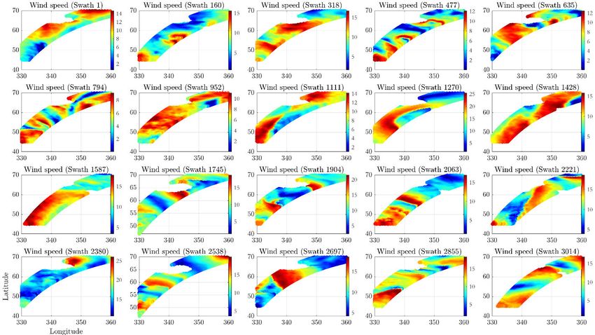
Introduction

Acknowledgement, motivation, related work
Acknowledgement
 ◦ Jon Tawn and Jenny Wadsworth (Lancaster), David Randell (Shell)
Motivation
 ◦ How useful are satellite observations of ocean waves and winds?
 ◦ Could they become the primary data source for decisions soon?
 ◦ What are the spatial characteristics of extremes from satellite
   observations?
Related work
 ◦ Heffernan and Tawn [2004] (CE), Heffernan and Resnick [2007]
 ◦ Shooter et al. [2019] (SCE), Wadsworth and Tawn [2019] (SCE)
 ◦ Shooter et al. [2021b], Shooter et al. [2021a] (SCE applications)
Competitors (= MSPs, hierarchical MSPs and multivariate MSPs)
 ◦ Reich and Shaby [2012], Vettori [2017], Vettori et al. [2019]
 ◦ Genton et al. [2015], Huser and Wadsworth [2020]
       Jonathan                       MSCE            September 2021   2 / 23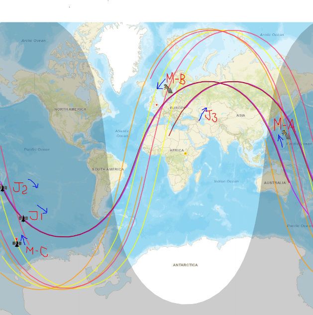
Introduction

Summary of talk : Outline

 ◦ A look at the data
 ◦ Brief overview of methodology, extended to multiple fields
 ◦ Results for joint spatial structure of extreme scatterometer wind
   speed, hindcast wind speed and hindcast significant wave height
   in the North Atlantic
 ◦ Implications for future practical applications

      Jonathan                      MSCE            September 2021   3 / 23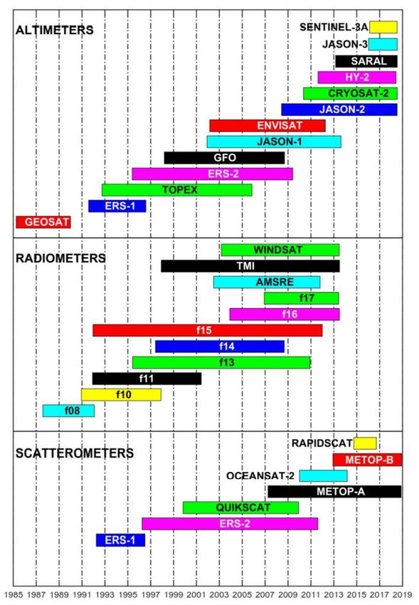
Introduction

Summary of talk : Methodology in nut-shell
                 ◦ Condition on large value x of first quantity X01 at
                   one location j = 0
                 ◦ Estimate “conditional spatial profiles” for m > 1
                                       p,m
                   quantities { X jk } j=1,k=1 at p > 0 other locations

                                          X jk ∼ Lpl
                                            x>u
                                 X |{ X01 = x} = α x + xβ Z
                               Z ∼ DL(µ , σ 2 , δ ; Σ(λ , ρ, κ ))
                 ◦ MCMC to estimate α , β, µ , σ , δ and ρ, κ , λ
                 ◦ α , β, µ , σ , δ spatially smooth for each quantity
                 ◦ Residual correlation Σ for conditional Gaussian
                   field, powered-exponential decay with distance

      Jonathan                   MSCE                    September 2021   4 / 23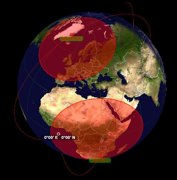
Data    Basics

Satellite observation
                                         Features
                                            ◦ Altimetry: HS and U10
                                            ◦ Scatterometry: best for U10 and
                                              direction
                                            ◦ > 30 years of observations
                                            ◦ Spatial coverage is by no means
                                              complete: one observation daily
                                              if all well
                                            ◦ Calibration necessary (to buoys
                                              and reanalysis datasets, Ribal
                                              and Young 2020)
                                            ◦ METOP(-A,-B,-C) since 2007
                                         HS : significant wave height (m)
         [Ribal and Young 2019]          U10 : wind speed (ms−1 ) at 10m (calibrated to 10-minute average
                                         wind speed)

      Jonathan                       MSCE                                 September 2021             5 / 23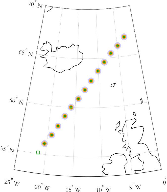
Data   Basics

Hindcast data, objectives
Hindcast data
  ◦ Physical simulator calibrated to observations (e.g from buoys)
  ◦ NORA10 hindcast covers North Atlantic off UK (Breivik et al.
     2013)
  ◦ Data available 1957-2018
Initial objective
  ◦ Joint spatial inferences about extremes using all of
      ◦ HS (JASON)
      ◦ directional U10 (METOP)
      ◦ directional HS and directional U10 (NORA10)
  ◦ Not feasible: poor joint spatial coverage of JASON and METOP
Revised objective
Joint spatial inferences about extremes of directional U10 (METOP),
hindcast directional HS and directional U10 (NORA10)
       Jonathan                   MSCE                September 2021   6 / 23
Data   Basics

JASON and METOP

  [n2yo.com, accessed 06.09.21 at around 1100UK]             [stltracker.github.io, accessed 27.08.2021 at around 1235UK]

 ◦ JASON and METOP similar polar orbits
 ◦ JASON all ascending, METOP all descending over North Atlantic
 ◦ Joint occurrence of JASON and METOP over North Atlantic rare
         Jonathan                                     MSCE                                 September 2021            7 / 23
Data Preprocessing
Swath wind speeds
Daily descending METOP swaths. Satellite swath location changes over time. Spatial structure evident
Jonathan MSCE September 2021 8 / 23Data Preprocessing
Registration locations
Procedure
◦ 14 longitude-latitude pairs
◦ Satellite observation nearest to
each pair used for each swath
◦ Corresponding hindcast data for
each pair at time of swath
◦ “Instantaneous” satellite wind
vector, hindcast wind vector,
hindcast HS and wave direction
for 1532 times
◦ Most southerly location for
conditioning in MSCE
Registration locations : square is conditioning location
◦ Note colour scheme
StlWnd (green), HndWnd (orange), HndWav(blue)
Jonathan MSCE September 2021 9 / 23Data Registered data
Scatter plots on physical scale
Scatter plots of registered data : StlWnd (green), HndWnd (orange), HndWav(blue)
Jonathan MSCE September 2021 10 / 23Data Registered data
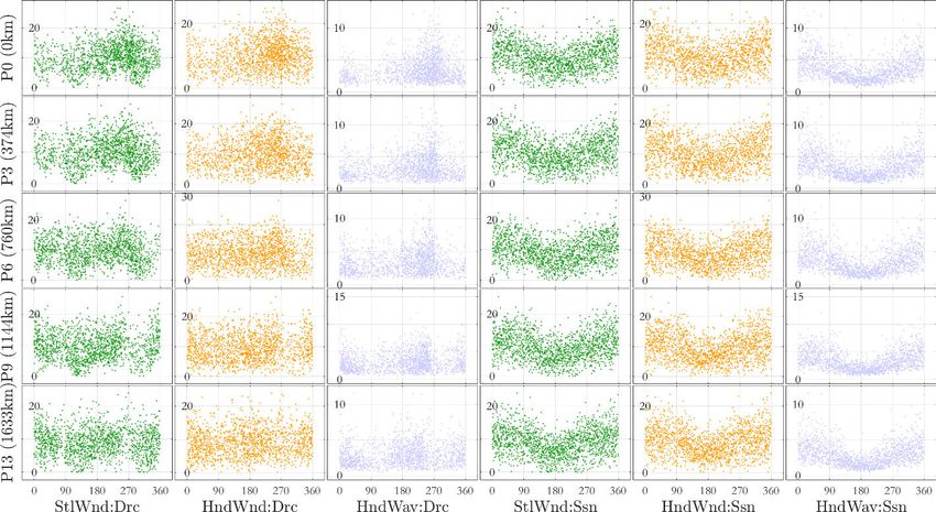
Covariate dependence
Directional and seasonal dependence. “Direction” is that from which fluid flows measured clockwise from North
StlWnd (green), HndWnd (orange), HndWav(blue)
Jonathan MSCE September 2021 11 / 23Data Marginal transformation to Laplace scale
Marginal transformation to standard Laplace scale
Procedure
◦ Non-stationary piecewise constant directional-seasonal marginal
extreme value model (github.com/ECSADES/ecsades-matlab)
◦ Pre-specified 8 directional bins (“octants”) of equal width centred
on cardinal and semi-cardinal directions
◦ Pre-specified “summer” and “winter” seasonal bins
◦ Generalised Pareto model for peaks over threshold
◦ Model parameters vary smoothly between bins, optimal
roughness found using cross-validation
◦ Multiple extreme value thresholds with non-exceedance
probabilities between 0.7 and 0.9 considered
◦ Bootstrapping for uncertainties
◦ Uncertainty in marginal model not propagated
◦ Independent marginal models for pair of variable (StlWnd,
HndWnd, HndWav) and location (0,1,...,13)
Jonathan MSCE September 2021 12 / 23Data Marginal transformation to Laplace scale
Scatter plots on Laplace scale
Registered data on Laplace scale: StlWnd (green), HndWnd (orange), HndWav(blue)
Jonathan MSCE September 2021 13 / 23Method Conditional extremes, CE
Conditional extremes
Y |{ X = x} = α x + xβ Z
◦ Asymptotically-motivated, Heffernan and Tawn [2004]
◦ X ∼ Lpl, Y ∼ Lpl, and x > u
◦ α ∈ [−1, 1], β ∈ (−∞, 1]
◦ Z is a residual random variable characterised empirically, or
estimated assuming Z ∼ N (µ , σ 2 ), so
E[Y |{ X = x}] = α x + µ xβ
var[Y |{ X = x}] = σ 2 x2β
◦ Identifiability of α and µ when β ≈ 1
◦ Model fitting means estimating α , β, µ and σ
Jonathan MSCE September 2021 14 / 23Method Spatial conditional extremes, SCE
Spatial conditional extremes
X |{ X0 = x} = α x + xβ Z
◦ Shooter et al. [2019], Wadsworth and Tawn [2019]
◦ X = ( X1 , X2 , ..., Xq ), are now observed at q points in space
◦ All marginal Xk ∼ Lpl, and x > u
◦ α j ∈ [−1, 1], β j ∈ (−∞, 1], j = 1, ..., q
Z ∼ DL(µ , σ 2 , δ ; Σ)
◦ Delta-Laplace (DL) parameters µ j , σ j > 0, δ j > 0, j = 1, ..., q
◦ Σ is a (conditional) correlation matrix with powered-exponential
decay with distance between the q points (with parameters ρ, κ )
◦ Model fitting means estimating α , β, µ , σ , δ and ρ, κ
◦ α , β, µ , σ , δ vary smoothly with distance
Jonathan MSCE September 2021 15 / 23Method Multivariate spatial conditional extremes, MSCE
Multivariate spatial conditional extremes
X |{ X01 = x} = α x + xβ Z
◦ X = ( X11 , X21 , ..., Xq1 , X12 , X22 , ..., Xq2 , ..., X1m , X2m , ..., Xqm ), for m
quantities observed at q points in space
◦ All marginal Xkℓ ∼ Lpl, and x > u
◦ α jℓ ∈ [−1, 1], β jℓ ∈ (−∞, 1], j = 1, ..., q, ℓ = 1, 2, ..., m
Z ∼ DL(µ , σ 2 , δ ; Σ)
◦ Delta-Laplace (DL) residual parameters µ jℓ , σ jℓ > 0, δ jℓ > 0
◦ Σ is a (conditional) correlation matrix with powered-exponential
decay with distance between the q points for m quantities, with
appropriate cross-decay (with parameters ρ, κ , λ)
◦ Model fitting means estimating α , β, µ , σ , δ and ρ, κ , λ
◦ α , β, µ , σ , δ vary smoothly with distance for each quantity
Jonathan MSCE September 2021 16 / 23Method Inference
Inference
◦ Adaptive MCMC, Roberts and Rosenthal [2009]
◦ Piecewise linear forms for all parameters with distance using nNod
spatial nodes
◦ Total of m(5nNod + (3m + 1)/2) parameters
◦ Rapid convergence, 10k iterations sufficient
Jonathan MSCE September 2021 17 / 23Results for North Atlantic Parameter estimates
Parameter estimates for North Atlantic application
Estimates for α , β, µ , σ and δ with distance, and residual process estimates ρ, κ and λ. Model fitted with τ = 0.75
StlWnd (green), HndWnd (orange), HndWav(blue)
Jonathan MSCE September 2021 18 / 23Results for North Atlantic Parameter estimates
Laplace-scale conditional mean, standard deviation
Quantile with threshold probability τ = 0.95 used for illustration. Quantile level is 2.3 at zero distance on green curve
StlWnd (green), HndWnd (orange), HndWav(blue)
Jonathan MSCE September 2021 19 / 23Results for North Atlantic Validation
Laplace-scale simulation under fitted model
Threshold probability τ = 0.75
Jonathan MSCE September 2021 20 / 23Results for North Atlantic Validation
Residual sample
◦ Black = From actual
sample
◦ Red = Simulated from
fitted model
Scatter matrix, threshold probability τ = 0.75
Jonathan MSCE September 2021 21 / 23Summary of findings
Summary of findings
Data
◦ JASON and METOP jointly too sparse to use together
◦ 1500-2000 good instantaneous daily observations for METOP
◦ Sampling bias; swath time roughly the same each day
◦ Data are “instantaneous” not storm peak
Methodology
◦ Inference straightforward for m = 3 and nNod = 10
◦ Assumed distance-dependence structure adopted, particularly for
residual, seems reasonable from diagnostics
◦ Marginal model (fitted independently, uncertainties not pushed
through to Laplace scale); should do this jointly
Results
◦ Results for threshold quantile τ = 0.75, other values examined
◦ Conditioning on other locations and quantities examined
◦ Spatial extent of extremal dependence for all quantities is about
600-800km
Jonathan MSCE September 2021 22 / 23References
References
O Breivik, O J Aarnes, J-R Bidlot, A Carrasco, and Oyvind Saetra. Wave extremes in the North East Atlantic from ensemble
forecasts. J. Climate, 26:7525–7540, 2013.
M. G. Genton, S. A. Padoan, and H. Sang. Multivariate max-stable spatial processes. Biometrika, 102:215–230, 2015.
J. E. Heffernan and S. I. Resnick. Limit laws for random vectors with an extreme component. Ann. Appl. Probab., 17:537–571, 2007.
J. E. Heffernan and J. A. Tawn. A conditional approach for multivariate extreme values. J. R. Statist. Soc. B, 66:497–546, 2004.
R. Huser and J. L. Wadsworth. Advances in statistical modelling of spatial extremes. Wiley Interdisciplinary Reviews: Computational
Statistics, 2020. doi: 10.1002/wics.1537.
Brian J. Reich and Benjamin A. Shaby. A hierarchical max-stable spatial model for extreme precipitation. Ann. Appl. Stat., 6:
1430–1451, 2012.
A. Ribal and I. R. Young. 33 years of globally calibrated wave height and wind speed data based on altimeter observations. Sci.
Data, 6:77, 2019.
A. Ribal and I. R. Young. Global calibration and error estimation of altimeter, scatterometer, and radiometer wind speed using
triple collocation. Remote Sens., 12:1997, 2020.
G. O. Roberts and J. S. Rosenthal. Examples of adaptive MCMC. J. Comp. Graph. Stat., 18:349–367, 2009.
R. Shooter, E. Ross, J. A. Tawn, and P. Jonathan. On spatial conditional extremes for ocean storm severity. Environmetrics, 30:
e2562, 2019.
R. Shooter, E Ross, A. Ribal, I. R. Young, and P. Jonathan. Spatial conditional extremes for significant wave height from satellite
altimetry. Environmetrics, 32:e2674, 2021a.
R Shooter, J A Tawn, E Ross, and P Jonathan. Basin-wide spatial conditional extremes for severe ocean storms. Extremes, 24:
241–265, 2021b.
S. Vettori. Models and Inference for Multivariate Spatial Extremes. KAUST Research Repository., 2017. URL
https://doi.org/10.25781/KAUST-G2PH8.
S. Vettori, R. Huser, and M. G. Genton. Bayesian modeling of air pollution extremes using nested multivariate max-stable
processes. Biometrics, 75:831–841, 2019.
J. L. Wadsworth and J. A. Tawn. Higher-dimensional spatial extremes via single-site conditioning. In submission,
arxiv.org/abs/1912.06560, 2019.
Jonathan MSCE September 2021 23 / 23You can also read