National Blend of Models: A Statistically Post-Processed Multi-Model Ensemble - DOI.org
←
→
Page content transcription
If your browser does not render page correctly, please read the page content below
Craven, J.P., D.E. Rudack, and P.E. Shafer, 2020: National Blend of Models: A statistically post-processed multi-model
                ensemble. J. Operational Meteor., 8 (1), 1-14, doi: https://doi.org/10.15191/nwajom.2020.0801

                         National Blend of Models: A Statistically
                          Post-Processed Multi-Model Ensemble
                                 JEFFREY P. CRAVEN, DAVID E. RUDACK, and PHILLIP E. SHAFER
                                     Meteorological Development Laboratory. Silver Spring, MD

                                    (Manuscript received 27 June 2019; review completed 22 October 2019)

                                                             ABSTRACT
      The National Blend of Models (NBM) is the culmination of an effort to develop a nationally consistent
    set of foundational gridded guidance products based on well-calibrated National Weather Service (NWS)
    and non-NWS model information. These guidance products are made available to the National Centers for
    Environmental Prediction centers and NWS Weather Forecast Offices for use in their forecast process. As
    the NWS continues to shift emphasis from production of forecast products to impact-based decision support
    services for core partners, the deterministic and probabilistic output from the NBM will become increasingly
    important as a starting point to the forecast process. The purpose of this manuscript is to document the progress
    of NBM versions 3.1 and 3.2 and what techniques are used to blend roughly 30 individual models and ensembles
    for a number of forecast elements and regions. Focus will be on the core elements such as (1) temperature and
    dew point temperature, (2) winter weather, fire weather, thunderstorm probabilities, and (3) wind speed and
    gusts.

1. Introduction                                                          blends (Gagan, 2009), which eventually led to the use
                                                                         of “AllBlend” for a common starting point for gridded
    The National Weather Service (NWS) has been                          Day 4-7 forecasts every 12 hours in 2011. AllBlend was
issuing gridded forecast products using the National                     a combination of 50% of the previous official NDFD
Digital Forecast Database (NDFD, Glahn and Ruth,                         forecast, and 50% of an equally weighted “consensus”
2003) for nearly two decades. During this time, there                    blend (CONSAll) of raw model (CONSRaw) and MOS
has been a gradual evolution from initializing gridded                   gridded (CONSMOS) forecasts. There were also bias
forecasts using individual models such as the North                      corrected (BC) versions of the above, where 30 day
American Mesoscale Model (NAM), the Global                               linear regression was used to adjust to a gridded ground
Forecast System (GFS), and GFS gridded model                             truth (BCCONSRaw, BCCONSMOS, BCCONSAll).
output statistics (MOS-GMOS) (Glahn et al. 2009) to                      Later, an improved blend (SuperBlend - Greif et al,
using blends of various guidance. This evolution was                     2017) was implemented and used as a starting point for
inspired by the success of using a consensus of models                   Day’s 2-7 forecast around 2016, using a combination of
(Vislocky and Fritsch, 1995; Baars and Mass, 2005;                       blended forecast inputs. The success of this project led to
Whitaker et al., 2006; Goerss 2007a) to produce more                     funding of the National Blend of Models (NBM) project
accurate forecasts. The National Hurricane Center has a                  in 2013. The Disaster Relief Appropriations Act of 2013
long history of using a consensus of numerical weather                   (commonly referred to as The Sandy Supplemental)
prediction (NWP) solutions to forecast the track of                      funded the NBM in 2013 to replace regional blends and
tropical cyclones and this has led to other similar efforts              create a nationally consistent starting point from which
within the NWS.                                                          grids could be adjusted as necessary.
    The NWS Central Region Gridded Methodology                               Early versions of the NBM were released in January
Advisory Team (CRGMAT) developed the consensus                           2016 (v1.0), November 2016 (v2.0), July 2017 (v3.0),

Corresponding author address: Jeffrey Craven, 1325 West East Highway, Room 10410, Silver Spring, MD, 20910
E-mail: jeffrey.craven@noaa.gov

                                                                     1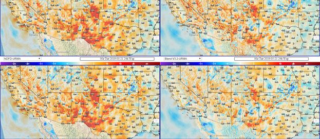
Craven et al.                              NWA Journal of Operational Meteorology                            21 January 2020

and October 2018 (v3.1). Development for v3.2 is                  of 7 new NWP inputs.
underway with expected implementation by November                     NBM v3.2 has six different forecast domains (see
2019. Each successive version is dedicated to adding              Fig. 1): (1) the CONUS at 2.5km, (2) Hawaii at 2.5km,
new weather elements and regions as required by the               (3) Alaska at 3km, (4) Puerto Rico at 1.25km, (5) Guam
National Service Programs (Stern, 2018). NBM v3.2 has             at 2.5km, and (6) the Oceanic Domain at 10km. NBM
six total regions (Contiguous United States {CONUS},              guidance is updated every hour at hourly time-steps for
Alaska, Hawaii, Guam, Puerto Rico, and Oceanic) and               projections 1-36, with 3-hourly projections between
65 weather elements.                                              39-192 hours, and finally 6-hourly projections between
     This manuscript will cover the techniques used               198-264 hours. Due to the sheer number of forecast
to produce most of the NBM elements except for                    elements and regions, we will not attempt to describe all
Probability of Precipitation (PoP) and Quantitative               of these to keep the length of the manuscript relatively
Precipitation Forecasts (QPF) (for that please see                concise.
Hamill et al., 2017 and Hamill and Scheuerer, 2018, for               A decaying average mean absolute error, Bt, is
details on quantile mapping and dressing).                        calculated each day for each member of the NBM by
                                                                  equation (1) where α is a predefined decaying weight
2. Data and methods                                               factor, FCSTt-1 is the most recent verifiable forecast,
                                                                  and OBSt-1, is its verifying observation. For the
    NBM v3.2 contains 31 different model systems                  NBM, the Real Time Mesoscale Analysis (RTMA) and
that are blended to produce a single deterministic                Unrestricted Real Time Mesoscale Analysis (URMA)
forecast product. For a growing number of elements,               (De Pondeca, 2011) are used as the ground truth
probabilistic forecasts are also created. Table 1 shows           observation.
the daily inputs of each of the 24 hourly runs. Inputs
from five different global modeling centers are present,                      Bt = (1-α) Bt-1 + α (FCSTt-1 - OBSt-1)        (1)
including USA National Centers for Environmental
Prediction      (NCEP),      Canadian      Meteorological         The decaying weight factor in equation (1) (using alpha
Center (CMC), Navy Fleet Numerical Operations                     setting of 0.05 in NBM v3.1) determines the dynamic
Center (FNMOC), European Center for Medium                        weighting value of the inputs (Cui et al, 2011). The final
Range Weather Forecasts (ECMWF), and Bureau of                    bias corrected forecast BCFCSTt is then simply defined
Meteorology (BoM) Australia. These span from high                 as the difference between the most recent forecast FCSTt
resolution convective allowing models such as the                 and the decaying average mean absolute error, Bt.
High Resolution Rapid Refresh (HRRR; Benjamin
et al, 2016), to global ensembles such as the Global                                  BCFCSTt = (FCSTt - Bt)                (2)
Ensemble Forecast System (GEFS; Zhou et al, 2017).
    The NBM cycle time does not refer to the cycle                The alpha setting in equation (1) was set to 0.05 for
times of the NWP cycle inputs but rather the cycle time           NBM v1.0, v2.0, v3.0, and v3.1, but was changed to
at which the NBM is run For example, an NBM run                   0.025 in NBM v3.2 for the 9 months of September
at 1200 Coordinated Universal Time (UTC) does not                 through May to more closely match values used by
include any NWP guidance from 1200 UTC. There is a                NCEP (alpha of 0.02) and research at MDL (Glahn,
data cutoff at forecast hour (HH) - 10, or in this example        2013). During the stagnant summer months of 2019
1150 UTC. The most recent model outputs available on              (June, July, August), the alpha setting of 0.05 had less
the Weather and Climate Operational Supercomputer                 mean absolute error (MAE) so that value (same as NBM
System (WCOSS) at 1150 UTC are included in the                    v3.1) will be left for those 3 months in v3.2 (which tend
1200 UTC NBM run. This includes both NCEP and                     to have less dramatic regime changes compared to the
non-NCEP NWP inputs; therefore, the 1200 UTC                      colder months of the year).
NBM contains several 0000 UTC and 0600 UTC inputs                    A detailed discussion of the tradeoff of bias/variance
(details can be found in Table 1). For each subsequent            when using exponentially weighted decaying average
hour the NBM is run there are at least four new NWP               can be found in chapter 7 of Hamill, 2019. Use of the
inputs out of the total of 31 possible data sources, while        decaying average technique results in forecasts that
at 0700 UTC and 1900 UTC there are 10 new NWP                     can unrealistically vary from day to day and location
inputs. Over a 24-hour period, each hour has an average           to location, a consequence of the small training sample

ISSN 2325-6184, Vol. 8, No. 1                                 2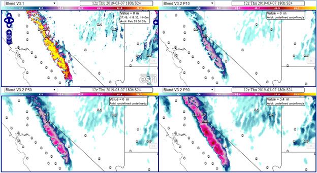
Craven et al.                                NWA Journal of Operational Meteorology                         21 January 2020

Table 1. The NBM v3.2 NWP inputs. * indicates inputs that provide wave model forecasts.
                                                                                                       Updates in NBM
    Model input                 Agency       Resolution             Cycles per day      Members
                                                                                                         cycle (UTC)
    ACCESS-R                BoM Australia        11 km                      4x               1            02, 08, 14, 20
    ACCESS-G                BoM Australia        35 km                      2x               1                07, 19
    ECMWFD*                   ECMWF              25 km                      2x               1                08, 20
    ECMWFE*                   ECMWF             100 km                      2x              50                09, 21
     EKDMOS                    NCEP             2.5 km                      4x               1            07, 11, 19, 23
       GDPS                 CMC Canada           25 km                      2x               1                05, 17
       GEPS                 CMC Canada           50 km                      2x              20                07, 19
      GEFS*                    NCEP              50 km                      4x              20            00, 06, 12, 18
       GFS*                    NCEP              13km                       4x               1            05, 11, 17, 23
       GLMP                    NCEP             2.5 km                     24x               1             Every hour
      GMOS                     NCEP             2.5 km                      2x               1                06, 18
    HiRes ARW                  NCEP               3 km                      2x               1                04, 16
    HiRes ARW2                 NCEP               3 km                      2x               1                04, 16
    HiRes NMM                  NCEP               3 km                      2x               1                04, 16
      HMON                     NCEP             1.5 km                      4x               1            00, 06, 12, 18
       HRRR                    NCEP               3 km                     24x               2             Every hour
      HWRF                     NCEP             1.5 km                      4x               1            00, 06, 12, 18
       NAM                     NCEP              12 km                      4x               1            03, 09, 15, 21
     NAMNest                   NCEP               3 km                      4x               1            03, 09, 15, 21
    NAVGEMD*                  FNMOC              50 km                      4x               1            00, 06, 12, 18
    NAVGEME*                  FNMOC              50 km                      2x              20                06, 18
        RAP                    NCEP              13 km                     24x               2             Every hour
       RDPS                 CMC Canada           10 km                      4x               1            04, 10, 16, 22
       REPS                 CMC Canada           15 km                      2x              20                07, 19
       SREF                    NCEP              16 km                      4x              24            01, 07, 13, 19

                                                                    size (especially as alpha values become larger). A
                                                                    comparison of the impact of bias correction to recent
                                                                    observations (over the past 10, 20, or 30 days) can be
                                                                    found in Table 2. The relatively large alpha setting of
                                                                    NBM v3.1 (0.05) makes the bias correction behave
                                                                    more like 30 day linear regression bias corrected
                                                                    forecasts which are only influenced by the past 30 days
                                                                    of training data. Meanwhile, the alpha setting of 0.025
                                                                    incorporates only 54% of the signal from the past 30
                                                                    days and will correct the forecasts to a longer training
Figure 1. Domain maps from the six NBM sectors:                     sample.
CONUS (upper left), Alaska (upper center), Hawaii                        Bias corrected NWP with lower MAE is given
(upper right), Puerto Rico (lower left), Guam (lower                relatively high weights, while those with higher MAE
center), and Oceanic (lower right). Click image for an              are given correspondingly lower weights. These
external version; this applies to all figures and hereafter.        weights vary by weather element, grid point, cycle
                                                                    time, and forecast projection. Dynamic weighting
                                                                    is applied to maximum temperature, minimum

ISSN 2325-6184, Vol. 8, No. 1                                   3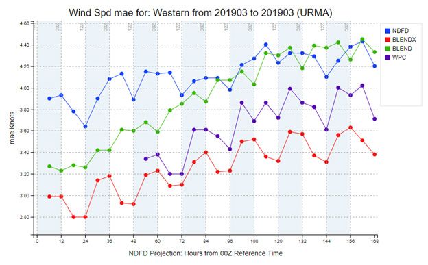
Craven et al.                              NWA Journal of Operational Meteorology                           21 January 2020

Table 2. A comparison of the impact of recent observations on bias correction in the past 30 days based on alpha
settings for exponentially weighted decaying average technique. Other linear regression based techniques used in
NWS WFOs blended forecasts are provided for comparison. The order is based on highest to lowest influence of
observations in the past 30 days.
                                  % influence Past 10              % influence Past 20            % influence Past 30
    Alpha Setting/Blend
                                         Days                             Days                           Days
           BCCONSAll                       33                                   67                         100
         0.05 (NBM v3.1)                   41                                   68                          85
        0.025 (NBM v3.2)                   23                                   41                          54
            0.02 (EMC)                     19                                   35                          48
            SuperBlend                     20                                   30                          45

temperature, temperature, dew point temperature, 10-m             among this group of core elements, but wind speed and
wind, 10-m wind gust, and significant wave heights.               gusts will be discussed in detail in a later section as the
These calculations are completed once per day using               bias correction process is more complex.
the most up-to-date URMA ground truth, and applied                     Maximum and minimum temperature and relative
to forecasts from 1 to 264 hours. 18-hour maximum                 humidity are initially calculated using 6-hour values
and minimum temperatures/humidity guidance is valid               available from the direct model output. If 6-hour
over a period while all other weather elements are valid          maximum/minimum values are not available, the
at an instant in time.. The NBM, RTMA/URMA, and                   highest or lowest hourly values during the period of
NWS Weather Forecast Offices (WFO) leverage the                   interest are used instead. Since URMA produces these
same high-resolution unified terrain data set to ensure           four parameters, the NBM bias corrects to the URMA
that all users of these data have an identical reference          values independent of the process of bias correction for
starting point (University Corporation for Atmospheric            hourly temperature and relative humidity. The definition
Research {UCAR}, 2016).                                           of these maximum/minimum fields is below:
     The bias correction of the various model inputs are
calculated and applied to each individual input. The bias           •       Maximum temperature is the 18-hour value
corrected forecast is then weighted based on the dynamic          		        from 1200 UTC to 0600 UTC (Day 2).
weightings, and combined for a final deterministic
forecast. The only exception to this process is sky cover,          •       Minimum temperature is the 18-hour value
where the MAE is used to assign dynamic weights                   		        from 0000 UTC to 1800 UTC.
although the sky cover inputs are not bias corrected.
We expect to bias correct sky cover using URMA after                •       Maximum relative humidity is the 12-hour
future upgrades when better nighttime first guess fields          		        value from 0600z UTC to 1800 UTC for most
from Geostationary Operational Environmental Satellite            		        sectors, and 1200 UTC to 0000 UTC (Day 2)
(GOES) 16/17 satellite imagery are incorporated into              		        for the Guam sector.
the URMA analysis. Table 3 provides a list of the 64
forecast elements that will be available with NBM v3.2.             •       Minimum relative humidity is the 12-hour
                                                                  		        value from 1800 UTC to 0600 UTC (Day 2) for
3. Analysis and Discussion                                        		        most sectors, and 0000 UTC to 1200 UTC for
                                                                  		        the Guam sector.
     a. The Core Elements
                                                                  Other derived parameters such as apparent temperature
    Elements related to temperature, dewpoint, relative           use the NBM temperature, dewpoint, and wind speed
humidity, and sky cover are examples of the core                  information to calculate the appropriate heat index or
elements where dynamic weighting based on MAE is                  wind chill values.
performed. They are calculated through 264 hours each                 Performance of the NBM is closely tracked using
hour by blending the bias corrected components. Wind              baselines of skill such as NDFD forecasts and GMOS
speed, wind direction, and wind gusts are often included          guidance. Bulk verification compares to URMA for

ISSN 2325-6184, Vol. 8, No. 1                                 4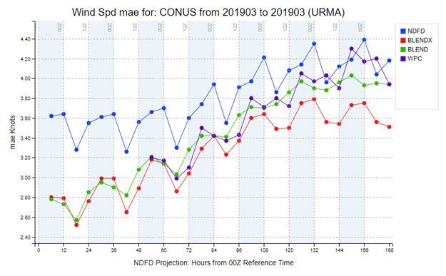
Craven et al.                                 NWA Journal of Operational Meteorology                                21 January 2020

Table 3. List of 64 forecast elements created for the NBM.
     Temp            Moisture      Precip           Wind                  Winter             Fire         Aviation         Marine
                   Relative
                                                10-m wind     Snow Amount                 Haines                          Sig Wave
 Temperature       Humidity     QPF 1 hour                                                              Sky Cover
                                                dir and speed 1 hour                      Index                           Height
                   (RH)
                                                10-m                 Snow Amount          Fosberg                         Freezing
 Max Temp          Max RH       QPF 6 hour                                                              Ceiling
                                                wind gust            6 hour               Index                           Spray
                                                30-m                 Snow Amount          Solar
 Min Temp          Min RH       QPF 12 hour                                                             Visibility        PMSL
                                                wind speed           24 hour              Radiation
 Apparent          Dew Point                    80-m                 Ice Amount           Mixing        Lowest
                                QPF 24 hour
 Temp              Temp                         wind speed           1 hour               Height        Cloud Base
                                Precipitation                        Ice Amount           Transport
 Water Temp                                                                                             Echo Tops
                                Duration                             6 hour               wind
                                                                     Ice Amount 24        Ventilation
                                PoP01                                                                   VIL
                                                                     hour                 Rate
                                                                     Cond prob of         3 hour prob   Max Hourly
                                PoP06
                                                                     Snow                 of Thunder    Reflectivity
                                                                                                        LLWS Dir
                                PoP12                                Cond prob of Rain
                                                                                                        and Speed
                                Predominant                                                             LLWS
                                                                     Cond prob of Sleet
                                Weather                                                                 Height
                                                                     Cond prob of
                                                                                                        Elrod Index
                                                                     Freezing Rain
                                                                                                        Mountain
                                                                     Cond prob of
                                                                                                        Wave
                                                                     refreezing sleet
                                                                                                        Turbulence
                                                                     Probability of ice
                                                                                                        SBCAPE
                                                                     present
                                                                                                        1 hour prob
                                                                     Max Tw aloft
                                                                                                        of t-storm
                                                                     Pos Energy of
                                                                                                        3 hour prob
                                                                     Warm Layer
                                                                                                        of t-storm
                                                                     (Bourgouin)
                                                                     Neg Energy of
                                                                                                        12 hour prob
                                                                     Cold Layer (Bour-
                                                                                                        of t-storm
                                                                     gouin)
                                                                     Snow Level
                                                                     Snow to liquid
                                                                     ratio

gridded forecasts at about 3.7 million grid points for the            NDFD from the 11-month period of October 2018
CONUS. URMA is used as the gridded analysis of truth                  through August 2019. Figure 2b is the same, except for
to which all gridded guidance and forecasts are verified              station-based verification versus METARs. Whether
against. To evaluate the performance of NBM guidance                  using URMA or METAR data as ground truth, the MAE
at select stations, primarily for Terminal Aerodrome                  for the NBM is lower than GFS MOS and GMOS.
Forecasts (TAFs), 1,319 Meteorological Terminal                            Figures 2c and 2d also indicate that the surface
Aviation Routine (METAR) stations are also used for                   temperature bias of the NBM is close to zero, even
verification. Figure 2a shows gridded temperature                     when compared to either GFS MOS or GMOS.
verification versus URMA for NBM, GMOS, and                           Results for dew point temperature, relative humidity,

ISSN 2325-6184, Vol. 8, No. 1                                    5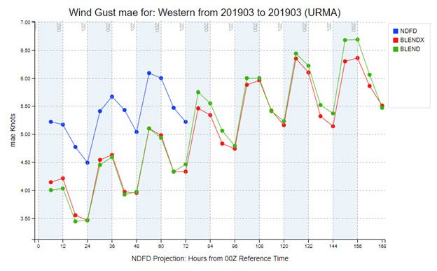
Craven et al.                              NWA Journal of Operational Meteorology                          21 January 2020

                                                        A                                                               B

                                                        C                                                               D

Figure 2. (A) Gridded temperature verification versus URMA for NBM (BLEND), GMOS, and NDFD from the
eleven month period October 2018 to August 2019. (B) As in Fig. 2a, except using 1319 CONUS METARs as
ground truth. (C) As in Fig. 2a, except for temperature bias. (D) As in Fig. 2a, except for temperature bias.

and significant wave height (not shown) also show                 projections. Figures 3a-3j compare MAE scores (Heidke
bias values near zero. This is one of the advantages of           Skill Score for Sky Cover and Brier Score for PoP12)
performing bias correction to observations in real-time           between NBM and GMOS for the period March 2017 to
– an inherent advantage that MOS guidance does not                August 2019 for the CONUS domain using URMA as
possess.                                                          ground truth. With hourly updates, the NBM provides
     Table 4 shows a matrix of relative performance               an excellent starting point for deterministic forecasts by
versus NDFD of the Day 1-3 NBM forecasts for                      incorporating the most recent NWP.
the meteorological winter months of December
2018-February 2019. Although performance is                           b. Fire Weather Elements
comparable for the CONUS, the NBM shows much
better skill for the outside the CONUS (OCONUS)                       The Fire Weather Program is one of 11 National
areas of Alaska, Hawaii, and Puerto Rico. Analogous               Service Programs in the NWS. A set of requirements for
results are found for Days 4-7 (Table 5). When using              gridded forecasts from NBM to support Fire Weather
URMA as ground truth, the error statistics heavily favor          related forecasts, watches, and warnings were provided
the NBM rather than the NDFD. However, the error                  and can be found in Table 3. There are a total of 12
statistics are similar when compared with point-based             elements from a combination of core elements and fire
METAR observations. Although these METAR-based                    weather elements. The primary inputs are temperature,
stats at 1,319 stations only represent about 0.04% of the         relative humidity, wind speed, and mixing height.
total grid points, they are representative of populated               Mixing height represents the top of the planetary
areas and airports.                                               boundary layer (PBL) and is calculated using a modified
     The NBM accuracy is far better than GMOS for                 Stull Method (Stull, 1991). Some of the 11 total fire
nearly every element in every sector at all forecast              weather NBM inputs influence or are associated with

ISSN 2325-6184, Vol. 8, No. 1                                 6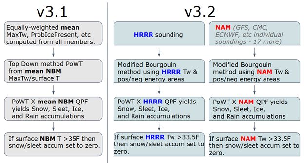
Craven et al.                                  NWA Journal of Operational Meteorology                         21 January 2020

Table 4. Relative performance of NBM v3.1 for December 2018 to February 2019 for the CONUS, Alaska (AK),
Hawaii (HI), and Puerto Rico (PR) versus NDFD for Day 1-3 forecasts. Ground truth is station based against
METAR (left columns) or gridded versus URMA (right columns). Much better is 10%+ improvement, better is
5-9% improvement, and similar is within + or - 4%.
                  CONUS         CONUS    AK      AK      HI            HI       PR         PR
    Day 1-3
                  METAR         URMA    METAR   URMA    METAR         URMA     METAR      URMA
    MaxT
    MinT
    Temp
      Td                                                                                                      NBM Much Better
     RH                                                                                                       NBM Better
    PoP12                                                                                                     Similar
  QPF06HSS                                                                                                    NDFD Better
  QPF06CSI                                                                                                    NDFD Much Better
   Snow06                                                                                                     N/A
     Sky
   WindDir
  WindSpeed
   WindGust
  Wave Height

Table 5. As in Table 4, except for Day 4-7 forecasts.
                  CONUS         CONUS    AK      AK      HI            HI       PR         PR
    Day 4-7
                  METAR         URMA    METAR   URMA    METAR         URMA     METAR      URMA
    MaxT
    MinT
    Temp                                                                                                      NBM Much Better
      Td                                                                                                      NBM Better
     RH                                                                                                       Similar
    PoP12                                                                                                     NDFD Better
     Sky                                                                                                      NDFD Much Better
   WindDir                                                                                                    N/A
  WindSpeed
  Wave Height

PBL height, which is also a reasonable estimate of                    transport wind yields the ventilation rate, which is used
the mixing height. An inventory of the lowest few                     to estimate the dispersion rate of smoke.
kilometers of the model sounding information was taken                    The lower atmosphere stability index or Haines
to determine which models had sufficient resolution                   Index (Haines, 1988) is also calculated using one of
to either calculate the Stull Method or provide a PBL                 three calculations (low, middle, and high). Utilizing
height. Transport wind speed is the average wind                      the 2.5km unified terrain height as reference, the NBM
magnitude in the layer defined by the surface and the                 calculates the Haines Index using the low equation for
mixing height. Transport wind direction is determined                 elevations below 1,000 ft mean sea level (MSL), the
by the vector of average U (zonal velocity) and average               middle equation for elevations from 1,000 to 2,999 ft
V (meridional velocity) wind components in that same                  MSL, and the high equation for elevations of 3,000
mixed layer. The product of the mixing height and the                 ft MSL and above. The Fosberg Index (1978) is also

ISSN 2325-6184, Vol. 8, No. 1                                     7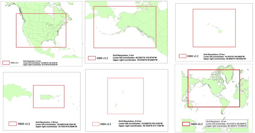
Craven et al.                             NWA Journal of Operational Meteorology                           21 January 2020

                                   A                                                 B                                   C

                                   D                                                 E                                   F

                                   G                                                 H                                    I

                                                                                     J
Figure 3. (A) Plot of maximum temperature MAE of NBM (Blend) in red and GMOS in blue for CONUS sector
using URMA as ground truth for period of March 2017 to August 2019. (B) As in Fig. 3a, except for minimum
temperature. (C) As in Fig. 3a, except for hourly temperature. (D) As in Fig. 3a, except for dew point temperature.
(E) As in Fig. 3a, except for heidke skill score for sky cover. (F) As in Fig. 3a, except for brier score for PoP12.
(G)As in Fig. 3e, except for QPF06. (H) As in Fig. 3a, except for wind direction. (I) As in Fig. 3a, except for wind
speed. (J) As in Fig. 3a, except for wind gust.

calculated, using a combination of temperature, relative          c. Winter Weather and Probability of Weather
humidity, and wind speed. Rather than calculating                		Types
a Fosberg Index for each model and then blending
those values to yield a final blended Fosberg Index,                 Deterministic snow and ice forecasts for 1-hour
the blended Fosberg Index is calculated by using its             and 6-hour amounts were introduced for the CONUS
blended input variables.                                         and Alaska domains beginning with NBM v3.1. At that
                                                                 time, probabilities of rain, snow, sleet, and freezing rain
                                                                 (Probability of Weather Type - PoWT) were derived
                                                                 via a “top-down” approach employed by the NWS
                                                                 Central Region “Forecast Builder” application. This

ISSN 2325-6184, Vol. 8, No. 1                                8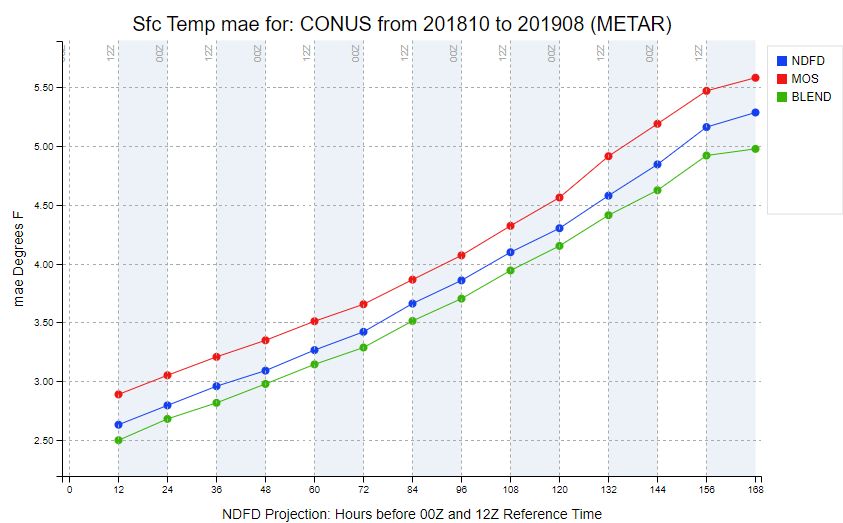
Craven et al.                              NWA Journal of Operational Meteorology                           21 January 2020

methodology assessed the presence of cloud ice in the             snow and ice amounts are computed individually
precipitating cloud layer (ProbIcePresent), the elevated          for each model and then combined with expert
warm layer aloft (maximum value of web bulb potential             weights to obtain blended deterministic snow and ice
temperature - MaxTw), and the surface-based cold                  accumulations. A comparison of PoWT and snow/ice
layer (see Baumgardt et al. 2017 for more details). The           amount methodologies for v3.1 and v3.2 is illustrated
probabilities were based on a mean sounding consisting            in Fig. 4. Results for the v3.2 methodology seen during
of 18 NWP inputs. Snow and ice amounts were                       the 2018-19 winter season showed some significant
derived by parsing the NBM deterministic mean QPF                 improvements, which include:
into amounts for each type based on their respective
PoWT ratios, and applying an equally-weighted mean                    1) More realistic gradients in PoWT.
snow-liquid ratio (SLR) and various NBM surface
temperature thresholds. The “top-down” methodology                  2)      A decrease in mean absolute error for 6-hour
was a good first step in providing deterministic snow             		        snow amount by up to 10% when subjectively
and ice amounts in the NBM, but came with some                    		        verified against the National Operational
drawbacks. The use of a mean sounding to derive                   		        Hydrologic Remote Sensing Center (NOHRSC)
PoWT resulted in sharp discontinuities in probabilities           		        snowfall analysis during several events.
near the surface freezing line and occasionally produced
extremely sharp gradients in snow accumulations. Also,              3) Improved snow forecasts around the snow level
an adjustment based on ProbIcePresent was assigning               		 in complex terrain and in rain/snow transition
too much QPF to freezing drizzle especially in the dry            		zones.
slots of storms. This type of diagnosis does not fully
account for important physical aspects of the thermal                In order to support a NWS probabilistic snow
profiles - namely the depth of the melting and refreezing         experiment, a variety of snow and ice percentiles
layers.                                                           and threshold probabilities were developed for v3.2
    For NBM v3.2, three important changes were                    covering 24-, 48-, and 72-hour periods. These include:
made. PoWT is now derived using a revised Bourgouin
layer energy technique which calculates areas of                    (1) 5th, 10th, 25th, 50th, 75th, 90th, and 95th
positive melting energy and negative refreezing energy            		 percentile snow amount
from the wet-bulb temperature profile, to determine
the likelihood of rain vs. snow and freezing rain                   (2) 5th, 10th, 25th, 50th, 75th, 90th, and 95th
vs. ice pellets (see Lenning and Birk 2018 for more               		 percentile ice amount
details). Probabilities are computed for each model
individually based on relationships derived from local              (3) Probability of exceedance for snowfall 0.1, 1,
studies (e.g., Lenning and Birk 2018), and an expert-             		 2, 4, 6, 8, 12, 18, 24, and 30 inches
weighted average is calculated from all model inputs
(18 inputs in short-term and 8 inputs in extended) to               (4) Probability of exceedance for ice 0.01, 0.1,
produce a blended PoWT. Similarly, 1-hour and 6-hour              		 0.25, 0.5, and 1.0 inches

                                                                  The percentiles and threshold probabilities listed above
                                                                  are computed directly from the ranked membership
                                                                  without assuming a particular distribution. To increase
                                                                  spread in the extended range, the membership was
                                                                  supplemented with seven additional inputs derived using
                                                                  the 5th, 10th, 25th, 50th, 75th, 90th, and 95th percentiles
                                                                  of NBM QPF. An example forecast of 10th, 50th, and
                                                                  90th percentile snow amount is shown in Fig. 5 for an
                                                                  event in the Sierra Nevada Mountains. Compared to
                                                                  v3.1 mean snowfall (top-left), the percentiles are more
                                                                  realistic and more closely match the amount observed
Figure 4. Comparison of PoWT and snow/ice amount                  at Lake Tahoe with this event (6-10” range).
methodologies for NBM v3.1 vs. v3.2.

ISSN 2325-6184, Vol. 8, No. 1                                 9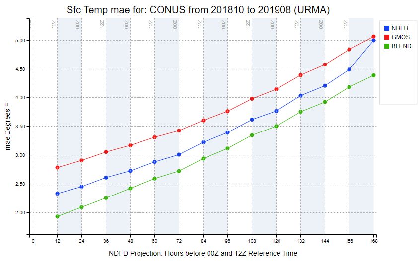
Craven et al.                              NWA Journal of Operational Meteorology                             21 January 2020

                                                                  		 weighted 50% for 1-h ProbThunder, which is
                                                                  		 expected to result in improved skill and spatial
                                                                  		 detail compared to the operational v3.1 SREF-
                                                                  		only product.

                                                                    (2)     New membership for 3-h/12-h ProbThunder -
                                                                  		        CONUS. Recently refreshed GFS MOS, NAM
                                                                  		        MOS, and ECMWF MOS components were
                                                                  		        developed and added to the membership for
                                                                  		        3-h and 12-h ProbThunder over the CONUS.
                                                                  		        The new MOS systems use total lightning
Figure 5. Example 180-hour NBM forecast of snow                   		        (in-cloud and CG) data to define the occurrence
amount percentiles, showing v3.1 mean snowfall                    		        of a thunderstorm in a 40-km grid box, and
(top-left), v3.2 10th percentile (top-right), v3.2 50th           		        use climatology and various model-derived
percentile (bottom-left), and v3.2 90th percentile                		        parameters as predictors (see Shafer and
(bottom-right).                                                   		        Rudack 2015 for a more detailed description of
                                                                  		        a typical MOS development for probability of
     d. Probability of Thunderstorms                              		        thunder). Aviation customers are also concerned
                                                                  		        with in-cloud (IC) lightning and not just CG,
    Guidance for the probability of a thunderstorm                		        thus the switch to a total lightning definition for
(hereafter “ProbThunder”) for 3-hour periods out to 84            		        the MOS components will result in a blended
hours over the CONUS was introduced in NBM v3.0 and               		        product that better serves aviation users.
was comprised only of Short Range Ensemble Forecast
(SREF)-based calibrated thunderstorm probabilities                    e. Wind Speed and Wind Gust elements
produced on WCOSS by the Storm Prediction Center
(SPC) (see Bright et al. 2005 for more details on the                  To date, the NBM weights and bias corrects both
SREF-based product). In NBM v3.1, ProbThunder for                 wind speed and wind gusts unconditionally. That is to
3-h and 12-h periods through 84 hours for CONUS was               say, the bias correction factor (BCF) and mean absolute
produced from an expert-weighted blend of SREF-                   error weighting factor (MAEWF) (that is used to
based (SPC) probabilities and GFS-based GMOS                      correct today’s raw model guidance) is independent of
probabilities (e.g., Shafer and Gilbert 2008), with SREF          the magnitude of the wind speeds used in generating the
given 67% weight and GMOS 33% weight. The SREF                    BCF and MAEWF. In most instances this unconditional
and GMOS products both define the occurrence of a                 adjustment works quite well because wind speeds are
thunderstorm as one or more cloud-to-ground (CG)                  generally low. However, when windier situations do
flashes in a 40-km grid box. Additionally, SPC SREF-              occur there is no discernable signal in the BCF and
based calibrated thunderstorm probabilities for 1-h               MAEWF to appropriately bias correct these anomalous
periods out to 36 hours was added to NBM v3.1.                    wind speeds and those non-anomalous wind speeds
    For NBM v3.2, the following enhancements will be              immediately following the event. To resolve this issue,
implemented for ProbThunder:                                      we have begun stratifying the BCF and MAEWF into
                                                                  specific categories (Table 6) that correspond to specific
  (1)      New membership for 1-h ProbThunder -                   NWS wind hazard categories.
		         CONUS. Localized Aviation MOS Program                       Prior to binning the model forecasts we identify
		         (LAMP) 1-h probability of lightning through            areas of pronounced local terrain features such as ridge-
		         25 hours over the CONUS (described in Charba           tops at the NBM grid resolution by comparing the
		         et al. 2017) will be added as a component              elevation of each gridpoint to the average elevation in
		         for NBM 1-h ProbThunder. The LAMP product              its vicinity. We do so by subtracting the elevation at each
		         incorporates output from the HRRR, Multi-              grid point in the high resolution unified terrain data set
		         Radar Multi-Sensor (MRMS) and total lightning          from the same smoothed grid point at a coarser spatial
		         observations as predictors, providing enhanced         resolution of approximately 65 km (Fig. 6). Those
		         skill especially in the first 6-9 hours. The           raw model wind speeds collocated with grid points of
		         LAMP and SPC SREF products will each be

ISSN 2325-6184, Vol. 8, No. 1                                10
Craven et al. NWA Journal of Operational Meteorology 21 January 2020
Table 6. The five wind speed and wind gust categories (units of meters per second) for which BCF and MAEWF
are calculated and used to bias correct the most current raw model’s input guidance.
Category Name Low Bound High Bound
No Advisory 0 9.5 (21.2 mph)
Small Craft Advisory 9.5 (21.2 mph) 17 (38.02 mph)
Gale Warning 17 (38.02 mph) 24.5 (54.80 mph)
Storm Warning 24.5 (54.80 mph) 32.5 (72.7 mph)
Hurricane Force Wind Warning 32.5 (72.7 mph) N/A
speeds were inflated after all inputs were blended. This
methodology overall works well; however, there are
instances when the wind speeds over ridge tops were
unrealistically high. Extensive testing has demonstrated
that by inflating individual raw model wind speeds
prior to their blending and binning the wind speeds
before being bias corrected removes the likelihood of
Figure 6. Schematic diagram of identifying areas of this scenario occurring.
pronounced terrain for inflating wind speeds. Essentially, the algorithm works in the following
manner for each input model cycle, projection, and
gridpoint: First, the raw wind speed is inflated using
pronounced terrain differences are inflated by a formula
the same methodology as in v3.1 in areas of higher
arrived at through empirical testing.
terrain. In areas where terrain is a nonissue the raw
wind speeds are unaltered. Raw wind gusts are not
Inflated Wind Speed = β WG * WG + (1 - β WG) * WS (3)
inflated irrespective of terrain. Second, these (inflated)
wind speeds (or wind gusts) are sampled and placed
Where β WG = Weight assigned to the wind gust
into one of five bins. Third, for a specific category,
the BCF and MAEWF is updated based upon the most
WG = Raw model wind gust after interpolation to
recent URMA observation. Only the wind speed (wind
NBM grid
gust) for that category is updated with new values - all
other categories remain unchanged. In this way, only
WS = Raw model wind speed after interpolation to
wind speeds (wind gusts) with specific thresholds
NBM grid
are modified and do not adversely affect the future
corrections of the remaining wind speeds (wind gusts)
Where β WG = (For TDIFF > 50 Meters) = Minimum
categories. Fourth, all bias corrected wind speeds (wind
(1,TDIFF/200)
gusts) are then weighed against all other inputs and then
blended. Stratifying in this manner will likely not only
β WG = (For TDIFF < 50 Meters) = 0
benefit the calibration of windier events but also benefit
the calibration of non-anomalous wind conditions that
and TDIFF = (High Resolution Elevation-Low
immediately follow.
Resolution Elevation)
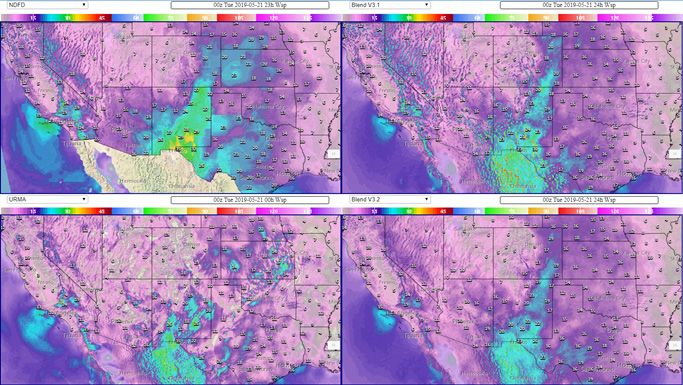
Figure 7 shows NDFD, NBM v3.1, NBM v3.2,
10 m wind, 24-hour forecasts issued on May 20,
We inflate wind speeds in areas of pronounced terrain
2019, alongside the verifying URMA analysis for the
by the model’s raw wind gust through a weighting
southwestern United States. While this wind event is
factor β WG. β WG is determined by a minimum function
not significant it does demonstrate that the NBM v3.2
yielding one of two possible values: (1) the ratio of the
wind speeds are more muted than NBM v3.1 over the
model terrain difference to a factor of 200 or (2) the
ridge tops in the Sierra Cascades. The verifying URMA
value of 1. The smaller of the two values is assigned
analysis difference fields shown in Fig. 8 (upper two
to β W to that grid point and the inflated wind speed
panels and lower right panel in Fig. 8) underscores
is calculated using equation (3). In NBM v3.1 wind
this point by highlighting the smaller wind speed
ISSN 2325-6184, Vol. 8, No. 1 11Craven et al. NWA Journal of Operational Meteorology 21 January 2020
Figure 7. May 20, 2019, 24-hour, 10 m wind speed A
forecasts in the Southwest United States for NDFD
(upper left), NBM v3.1 (upper right), NBM v3.2 (lower
right), and the verifying URMA analysis (lower left).
B
Figure 8. Forecast-Analysis difference fields for
24-hour, 10 m wind speed forecasts shown in Fig. 7
using the verifying URMA analysis valid 0000 UTC
May 21 2019.
differences with lighter colors in the lower right panel
when compared to the two upper panels. Similar results
are noted for wind gust forecasts (not shown).
Bulk NBM v3.2 10 m wind speed MAE
verification for March 2019 for both the CONUS and C
western CONUS (Fig. 9a and 9b) also shows a notable
Figure 9. (A) MAE bulk verification scores for 10
improvement in scores over NBM v3.1 especially in the
m wind speed for the United States for March 2019
medium range. NBM v.3.1 10 m wind gust verification
forecasts valid at 0000 UTC. In the legends below,
for March 2019 also demonstrates an improvement over
“BLEND” refers to NBM v3.1 and “BLENDX” refers
NBM v.3.1 for the western CONUS (Fig. 9c). However,
to NBM v3.2. (B) Same as Fig. 9a except for the western
the CONUS-wide verification for 10 m wind gusts are
United States. (C) Same as Fig. 9b except for wind gust.
more mixed (not shown) with NBM v3.1 still generally
displaying better MAE (on the order of 0.2-0.4 kt) in the
medium range. The improvement of NBM wind speed and will continue to improve the accuracy of NBM
and wind gust guidance can likely be attributed to a wind speeds and wind gusts.
combination of modifying the terrain-inflation of wind
speeds and stratifying the bias correction and MAE 4. Conclusions
weighting of wind speeds and wind gusts. With future
adequate sampling of the windier months of fall, winter, Blending high-resolution URMA bias-corrected
and spring, we believe the binning methodology will multi-model deterministic and ensemble-based
become a more influential component of this algorithm guidance produces more skillful guidance than NDFD
ISSN 2325-6184, Vol. 8, No. 1 12Craven et al. NWA Journal of Operational Meteorology 21 January 2020
forecasts in both gridded and station based verification. REFERENCES
The process of downscaling information from coarser
global models adds detail in areas of complex terrain. Baumgardt, D., Just A., and P. E. Shafer, 2017: Deriving
The NBM updates each hour with the latest NWP precipitation type probabilities in the National Blend
information. Although historically we have had forecast of Models. Poster, 28th Conference on Weather Analysis
and Forecasting / 24th Conference on Numerical Weather
packages that are updated two to four times per day, the
Prediction, Seattle, WA, Amer. Meteor. Soc., CrossRef.
NBM acts as a flywheel of forecast information that is Benjamin, S. G., and Coauthors, 2016: A North American
constantly refreshing and updating during the course of hourly assimilation and model forecast cycle: The Rapid
a day. Refresh. Mon. Wea. Rev., 144, 1669–1694, CrossRef.
Although the NBM does perform well in Baars, J. A, and C. F. Mass, 2005: Performance of National
deterministic forecasts, the real power of multi-model Weather Service forecasts compared to operational,
ensembles and post processing is the ability to produce consensus, and weighted Model Output Statistics, Wea.
calibrated probabilistic information for use in Impact- Forecasting, 20,1034-1047, CrossRef.
Based Decision Support Services. There is uncertainty Bright, D.R., Wandishin, M.S., Jewell, R.E., Weiss, S.J.,
in every forecast, and it is difficult to produce a 2005. A physically based parameter for lightning
deterministic forecast that represents all the potential prediction and its calibration in ensemble forecasts.
outcomes. Providing more information about the most Preprints, Conf. on Meteo. Appl. of Lightning Data. San
Diego, CA, Amer. Meteor. Soc., 4.3. CrossRef.
likely scenarios and potential alternative outcomes
Charba, J. P., F. G. Samplatsky, P. E. Shafer, J. E. Ghirardelli,
should help core customers make better decisions. and A. J. Kochenash, 2017: Experimental upgraded
LAMP convection and total lightning probability
Acknowledgments: A special thanks to Robert and “potential” guidance for the CONUS. Preprints, 18th
James, Eric Engle, Carly Buxton, Cassie Stearns, Conference on Aviation, Range, and Aerospace
Michael Baker, Daniel Nielson, and Scott Scallion Meteorology, Seattle, WA, Amer. Meteor. Soc., 2.4.
to their major contributions to the WCOSS code. We CrossRef.
thank the two thorough anonymous reviewers of the Cui, B., Z. Toth, Y. Zhu, and D. Hou, 2011: Bias correction
manuscript and their many useful suggestions that for global ensemble forecast, Wea. Forecasting, 27,396-
improved the content.. Thanks also to Bruce Veenhuis, 410, CrossRef.
Tamarah Curtis, Geoff Wagner, Andrew Benjamin, De Pondeca, M. S. F, G. S. Manikin, G. DiMego, S. G.
Justin Wilkerson, Yun Fan, Christina Finan, James Benjamin, D. F. Parrish, R. J. Purser, W.S. Wu, J. D. Horel,
D. T. Myrick, Y. Lin, R. M. Aune, D. Keyers, B. Colman,
Su, and Wei Yan for their contributions to the code.
G. Mann, and J. Vavra, 2011. The Real-Time Mesoscale
We also thank a great deal of subject matter experts Analysis at NOAA’s National Centers for Environmental
and contributors (far too many to list in total): John Prediction: Current status and development. Wea.
Wagner, Tabitha Huntemann, Dana Strom, Linden Wolf, Forecasting, 26, 593-612. CrossRef.
Brian Miretzky, Kathyrn Gilbert, David Ruth, David Fosberg, M. A., 1978: Weather in wildland fire management:
Myrick, David Novak, James Nelson, Mark Klein, The fire weather index. Conference on Sierra Nevada
Jerry Wiedenfeld, Andrew Just, Dan Baumgardt, Eric Meteorology, pp. 1-4, June 19-21 Lake Tahoe, CA.
Lenning, Kevin Birk, Matthew Jeglum, the members of Gagan, J., C. Greif, G. Izzo, J. P. Craven, J. Martin, J. Green,
the NBM Science Advisory Group, the Nation Service M. Kreller, R. Khron, R. Berdes, 2009: NWS Central
Program Leads and Teams, Darren Van Cleave, the Region Grid Methodology Advisory Team Final Team
NWS Regional Scientific Services Divisions, Bob Report, NWS CRH Scientific Services Division, 17 pp.
Glahn, Stephan Smith, William Bua, Ming Ji, and Chris Glahn, H. R and D. P. Ruth, 2003: The New Digital Forecast
Database of the National Weather Service. Bull. Amer.
Strager.
Meteor. Soc., 84, 195-202. CrossRef.
____, K. Gilbert, R. Cosgrove, D. P. Ruth, and K. Sheets,
_____________________ 2009. The Gridding of MOS. Wea. Forecasting, 24, 520-
529. CrossRef.
____, 2013. A comparison of two methods of bias correcting
MOS temperature and dewpoint forecasts. MDL Office
Note 13-1, 22 pp.
Goerss, J. S., 2007a: Prediction of consensus tropical cyclone
track forecast error. Mon. Wea. Rev., 135, 1985–1993.
CrossRef.
ISSN 2325-6184, Vol. 8, No. 1 13Craven et al. NWA Journal of Operational Meteorology 21 January 2020
Greif, C., J. Wiedenfeld, A. Just, 2017: Central Region
ForecastBuilder experiment summary report, NWS CRH
Scientific Services Division, 35 pp.
Haines, D.A. 1988. A lower atmospheric severity index for
wildland fires. Natl. Wea. Dig. 13(3): 23-27.
Hamill, T,M., E. Engle, D. Myrick, M. Peroutka, C. Finan,
and M. Scheurer, 2017: The U.S. National Blend of
Models for statistical postprocessing of probability of
precipitation and deterministic precipitation amounts,
Mon. Wea. Rev., 145, 3441-3463, CrossRef.
____, and Scheuerer, M., 2018: Probabilistic precipitation
forecast postprocessing using quantile mapping and
rank-weighted best-member dressing. Mon. Wea. Rev.,
146, 4079-4098. CrossRef.
____, 2019: Practical aspects of statistical postprocessing.
Statistical Postprocessing of Ensemble Forecasts, S.
Vannitsem, D. Wilks, and J. Messner, Eds., Elsevier,
187–217. CrossRef.
Lenning, E., and K. Birk, 2018: A revised Bourgouin
precipitation-type algorithm [Recorded Presentation].
29th Conference on Weather Analysis and Forecasting,
Denver, CO, Amer. Meteor. Soc., 3A.5. CrossRef.
Shafer, P. E., and K. K. Gilbert, 2008: Developing GFS-
based MOS thunderstorm guidance for Alaska. Preprints,
3rd Conference on Meteorological Applications of
Lightning Data, New Orleans, LA, Amer. Meteor. Soc.,
P2.9. CrossRef.
____, and D. E. Rudack, 2015: Development of a MOS
thunderstorm system for the ECMWF model. Seventh
Conference on the Meteorological Applications of
Lighting Data, Phoenix, AZ, Amer Meteor. Soc., 2.1.
CrossRef.
Stern, A. D., 2018: NWS Directives 10-102, Products and
services change management, 40 pp. CrossRef.
Stull, R. B., 1991: Static stability—an update. Bull. Am.
Meteor. Soc., 72, 1521–1529, CrossRef.
Univ. Corp. for Atmos. Research (UCAR), Cooperative
Program for Meteorological Education and Training,
2016: Unified Terrain in the National Blend of Models,
training module. CrossRef.
Vislocky, R. L., and J. M. Fritsch, 1995: Improved model
output statistics forecast through model consensus. Bull.
Amer. Meteor. Soc., 76, 1157–1164. CrossRef.
Whitaker, J.S., X. Wei, and F. Vitart, 2006: Improving week-
2 forecasts with multimodel reforecast ensembles. Mon.
Wea. Rev., 134, 2279–2284. CrossRef.
Zhou, X., Y. Zhu, D. Hou, Y. Luo, J. Peng, and R. Wobus,
2017: Performance of the New NCEP Global Ensemble
Forecast System in a parallel experiment. Wea.
Forecasting, 32, 1989-2004. CrossRef.
ISSN 2325-6184, Vol. 8, No. 1 14You can also read