OptTTA: Learnable Test-Time Augmentation for Source-Free Medical Image Segmentation Under Domain Shift
←
→
Page content transcription
If your browser does not render page correctly, please read the page content below

Proceedings of Machine Learning Research – Under Review:1–26, 2022                  Full Paper – MIDL 2022

OptTTA: Learnable Test-Time Augmentation for Source-Free
    Medical Image Segmentation Under Domain Shift

Devavrat Tomar1                                                            devavrat.tomar@epfl.ch
1
    Signal Processing Laboratory 5 (LTS5), EPFL, Switzerland
Guillaume Vray1                                                            guillaume.vray@epfl.ch
Jean-Philippe Thiran1,2,3,4                                      jean-philippe.thiran@epfl.ch
2
    University of Lausanne (UNIL), Switzerland
3
    Radiology Department, Centre Hospitalier Universitaire Vaudois (CHUV), Switzerland
Behzad Bozorgtabar1,3,4                                               behzad.bozorgtabar@epfl.ch
4
    Center for Biomedical Imaging (CIBM), Switzerland

Editors: Under Review for MIDL 2022

                                               Abstract
      As distribution shifts are inescapable in realistic clinical scenarios due to inconsistencies in
      imaging protocols, scanner vendors, and across different centers, well-trained deep models
      incur a domain generalization problem in unseen environments. Despite a myriad of model
      generalization techniques to circumvent this issue, their broad applicability is impeded as
      (i) source training data may not be accessible after deployment due to privacy regulations,
      (ii) the availability of adequate test domain samples is often impractical, and (iii) such
      model generalization methods are not well-calibrated, often making unreliable overconfident
      predictions. This paper proposes a novel learnable test-time augmentation, namely OptTTA,
      tailored specifically to alleviate large domain shifts for the source-free medical image
      segmentation task. OptTTA enables efficiently generating augmented views of test input,
      resembling the style of private source images and bridging a domain gap between training
      and test data. Our proposed method explores optimal learnable test-time augmentation
      sub-policies that provide lower predictive entropy and match the feature statistics stored in
      the BatchNorm layers of the pretrained source model without requiring access to training
      source samples. Thorough evaluation and ablation studies on challenging multi-center
      and multi-vendor MRI datasets of three anatomies have demonstrated the performance
      superiority of OptTTA over prior-arts test-time augmentation and model adaptation methods.
      Additionally, the generalization capabilities and effectiveness of OptTTA are evaluated
      in terms of aleatoric uncertainty and model calibration analyses. Our PyTorch code
      implementation is publicly available at https://github.com/devavratTomar/OptTTA.
      Keywords: Learnable test-time augmentation, domain shift, medical image segmentation

1. Introduction
The common assumption of most deep models used for medical image segmentation is that
training and test data distributions are alike. Nonetheless, this assumption can be easily
broken in real-world situations, and deep models might encounter performance degradation
when ported on a test environment that differs considerably from those used at training
time due to variations in imaging protocols, scanner vendors, etc. Thus, many recent
methods focus on improving model robustness trained on training data (a.k.a. source

© 2022 D. Tomar, G. Vray, J.-P. Thiran & B. Bozorgtabar.
Tomar Vray Thiran Bozorgtabar

domain) to generalize better in the new test environment (a.k.a. target domain). Several
techniques, including unsupervised domain adaptation (UDA) methods (Tomar et al., 2021b;
Vu et al., 2019; Chen et al., 2019b; Zhang et al., 2021; Bozorgtabar et al., 2019; Tomar
et al., 2021a), and domain generalization (DG) approaches (Li et al., 2020; Dou et al., 2019)
have been proposed; each formulates this problem differently. Nevertheless, there are still
substantial practical barriers to using these techniques in clinical practice. Prior UDA and
DG approaches require concurrent access to source and target samples or multiple source
domains, often infeasible after model deployment due to privacy regulations arising from
source data or when target data is scarce. Thus, a learning framework wherein only a
source model is required to adapt itself to a new target domain without the source data
is paramount for medical image segmentation. Recent methods have been proposed to
tackle this issue based on source-free domain adaptation (Liu et al., 2021; Bateson et al.,
2020) or test-time model adaptation (TTMA) (Sun et al., 2020; Nado et al., 2020). These
methods often utilize self-training schemes with entropy minimization (Wang et al., 2021;
Lee et al., 2013), test-time batch normalization (Nado et al., 2020), or additional auxiliary
training networks (He et al., 2020; Karani et al., 2021; Valvano et al., 2021). Despite
their practical success on minor domain shifts, those self-training techniques often produce
incorrect predictions in the presence of large domain shifts leading to error accumulation
during model adaptation as reported in previous works (Prabhu et al., 2021; Chen et al.,
2019a; Jiang et al., 2020). Recently, test-time augmentation (TTA) methods (Wang et al.,
2018; Isensee et al., 2018; Moshkov et al., 2020; Amiri et al., 2020; Wang et al., 2019)
have shown promise in improving robustness and accuracy without retraining the model
by aggregating predictions over multiple augmented versions of each test image. More
recently, inspired by training-time policy search approaches (Cubuk et al., 2019; Lim et al.,
2019; Hendrycks et al., 2020), test-time policy search methods (Lyzhov et al., 2020; Kim
et al., 2020; Shanmugam et al., 2021) have been proposed for classification tasks to find
static policies using either a greedy search algorithm (Lyzhov et al., 2020), an auxiliary
module (Kim et al., 2020) to predict sample-specific loss, or a learnable aggregation strategy
(Shanmugam et al., 2021). Nonetheless, they require policy search using a separate validation
set, and learned augmentation policies might not be optimal for each test sample.
Contributions. To the best of our knowledge, (i) we propose the first learnable TTA
policy, namely OptTTA, on the task of medical image segmentation tailored for alleviating
large domain shifts. (ii) Despite existing TTA methods based on static policies, OptTTA
dynamically selects optimal TTA policies producing transformed versions of test input,
resembling the style of private source training images. (iii) OptTTA can be implemented
in a streaming fashion via fine-tuning sub-policies sequentially for image volumes. (iv)
Experiments on challenging multi-center and multi-vendor MRI datasets of various anatomies
show OptTTA superiority against prior-arts. Further, we provide analyses for the TTA-based
aleatoric uncertainty and model calibration to support the effectiveness of OptTTA.

2. Methods
This section describes our proposed method, OptTTA, for learning TTA policy on medical
image segmentation under large domain shift using only a trained model on source data
without requiring access to neither training source data nor all target data at once during

                                              2
Learnable Test-Time Augmentation for Source-Free Medical Image Segmentation

            Pool of Sub-policies    Augmented views                                  Final Pool of
                                                           backprop
                                                                                     Sub-policies

                                                                                                           Exploration
                                                 ...

                                                                                                             Phase
                                                           backprop
                                                 ...                   Top-k
                                                                                            ...
                    ...                    ...
                                                           backprop
                                                 ...

                                                                                                           Exploitation
                                                                                              Ensembling

                                                                                                              Phase
              Test-Time              ...                                       ...
            Augmentation                                  Source
                                                       Trained Model

Figure 1: OptTTA involves two phases - (1) Exploration– All sub-policies in S are
          optimized using gradient descent followed by the selection of top-k sub-policies
          as T ∗ ; (2) Exploitation– The sub-policies of T ∗ are fine-tuned in streaming
          fashion for the rest of the target image volumes texploit , followed by ensembling the
          predictions of the source model over multiple transformations of the test image
          volume.

inference. As shown in Fig. 1, OptTTA involves two phases: (1) Exploration and (2)
Exploitation. In the Exploration phase, we search for data augmentation policies that
perform well based on the evaluation criterion mentioned in Sec. 2.2.1 using a set of target
image volumes texplore without any segmentation labels. Once we find the optimal data
augmentation policies in the Exploration phase, we fine-tune the same data augmentation
policies for the rest of the target image volumes texploit , one image volume at a time to
generate multiple augmented views. The predictions of the source trained model on these
optimal augmented views are then ensembled, yielding the final prediction. Here, we first
introduce the policy search space (Sec. 2.1) comprising data augmentation operations followed
by the TTA sub-policy evaluation criterion–LOptTTA without ground-truth segmentation
(Sec. 2.2.1). Finally, we describe a gradient-descent-based search algorithm for optimal TTA
sub-policies in Sec. 2.2.2.

2.1. Policy Search Space

Let O be a set of image transformation operations O : X → X on the image space X . In
particular, the list of transformations includes Identity (I), Gamma Correction (G), Gaussian
Blur (GB), Contrast (C), Brightness (B), Resize Crop (RC), Horizontal Flip (HF), Vertical Flip
(VF), Rotate (R). We parameterize each transformation O with its magnitude λ, sampled from
a probability distribution qθ with parameter θ. Some transformations in O (i.e. Horizontal
Flip, Vertical Flip, Rotate) do not have any learnable parameters. Let S be a set of

                                                       3
Tomar Vray Thiran Bozorgtabar

sub-policies, where a sub-policy τ ∈ S consists of Nτ consecutive transformation operations
from O : {Onτ (x; λτn ) : n = 1, ..., Nτ }, where each operation is applied sequentially as:

                                           xn = Onτ (xn−1 ; λτn )                          (1)
where x0 = x, xNτ = τ (x) and λτn ∼ qθnτ . An example of a sub-policy is [Resize Crop,
brightness, Horizontal Flip]. The final policy T is a collection of NT sub-policies.

2.2. Evaluating and Optimizing TTA Sub-Policies
2.2.1. Evaluation Criterion
The main essence of our method relies on the observation that a source trained model
outputs high confidence predictions (low entropy) and high accuracy for source-like images
that also match the feature statistics stored in the BatchNorm layers of the pretrained model.
Let X τ denote the set of 2D augmented views of the target image volume t generated using
a sub-policy τ ∈ S by sampling the magnitude λτn of its operations {Onτ } from a probability
distribution {qθnτ } with parameters {θnτ } using Eq. 1. We then define a test-time smoothing
loss function over the outputs of the segmentation model on X τ as follows:
                                   1 X
                  L(X τ ) =               Lent (x) + α1 Lbn (X τ ) − α2 Lcm (X τ )         (2)
                                 |X τ | τx∈X
where α1 and α2 are hyper-parameters, and the individual loss terms are described below.
BatchNorm Statistics Loss (Lbn ). This loss term acts as the feature distribution
regularizer to penalize the distance between the statistics of network activations on the
batch of augmented images X τ and that of the private source data stored in the widely-used
BatchNorm (BN) layers of the pretrained network.
                                    X                                                 2
                   Lbn (X τ ) =            ∥µl (X τ ) − µ̄l ∥22 + σl2 (X τ ) − σ̄l2   2
                                                                                           (3)
                                     l
where µl (X τ )and  σl2 (X τ )
                           are the batch-wise feature means and variances at the l-th BN
layer for an input batch of augmented images X τ , and µ̄l and σ̄l2 are the corresponding
mean and variance parameters stored in the l-th BN layer.
Conditional Entropy Loss (Lent ). This loss term is defined over the pixel predictions of
the segmentation model on the input image x and encourages high confidence predictions.
                                                  X
                                  Lent (x) = −          p(y|x) log p(y|x)                  (4)
                                                    y

where p(y|x) is the softmax output of the segmentation model on the input image x, and y
denotes model prediction spans over the segmentation classes.
Entropy of Class Marginals         (Lcm ) Maximizing this loss term encourages the model
predictions p̂(y) = |X1τ | x∈X τ p(y|x) to be uniformly distributed over the segmentation
                          P
classes as minimizing Eq. 4 alone may result in predictions converging to a single segmentation
class. Lcm does not require any prior information about the segmentation class distribution.
                                                        X
                                    Lcm (X τ ) = −          p̂(y) log p̂(y)                (5)
                                                        y

                                                        4
Learnable Test-Time Augmentation for Source-Free Medical Image Segmentation

2.2.2. Optimization Algorithm
A sub-policy τ is evaluated by taking the expectation of Eq. 2 with respect to the random
magnitudes of its augmentations. We then learn the distribution parameters θτ = {θnτ : n =
1, ..., Nτ } associated with a sub-policy τ that minimize this expected loss.

                              LτOptTTA (θτ , t) = EX τ ∼τ (t) [L(X τ )]                     (6)

For estimating the gradients of LτOptTTA with respect to its corresponding probability
distribution parameters θτ , we perform the re-parametrization trick by sampling magnitude
λτ from a Uniform distribution as follows:

                                    λτ ∼ µτ + σ τ · U(−1, 1)                                (7)

where θτ = {µτ , σ τ }, U(−1, 1) is Nτ dimensional Uniform distribution, and {µτ , σ τ } ∈ RNτ .
Thus, X τ becomes a function of (µτ , σ τ ) and the gradients of Eq. 6 are estimated as follows:
                                                τ
                                                ∇µ L(X(µτ , σ τ ))

                                  \ τ
                              ∇θτ LOptTTA =                                                  (8)
                                                ∇τσ L(X(µτ , σ τ ))
We use the AdamW (Loshchilov and Hutter, 2018) gradient descent approach to optimize
the parameters θτ of the sub-policy τ , summarized in the Algorithm (Appendix A).

2.3. Top-k Sub-Policies Selection and Test-Time Aggregation
During Exploration, we optimize every sub-policy in S using the Algorithm described
in Appendix A (Mode := explore) over target image volumes texplore and obtain the
corresponding set of optimized sub-policies S ∗ . We observe that some of the optimized
sub-policies in S ∗ perform poorly with a large loss LOptTTA . Thus, we dynamically keep top
k sub-policies from S ∗ having the k lowest loss values in the final policy set T ∗ using the
evaluation loss in Eq. 2 (cf. Table 5, Appendix D.2). In the Exploitation phase, we only
fine-tune the optimal sub-policies in T ∗ using Algorithm in Appendix A (Mode := exploit)
and generate augmented views of target image volumes texploit one at a time in a sequential
manner. For every sub-policy τi∗ ∈ T ∗ : i = 1, ..., k, we generate M augmented views of the
target image volume t and aggregate the predictions of the source trained model on these
views:
                                               k M
                                         1 XX                  τ∗
                               p̄(t) =                 p(yij |xj i )                       (9)
                                       k·M
                                                i=1 j=1
        τi∗     ∗
where xj ∈ X τi , which is sampled M times independently from sub-policy τi∗ .

3. Experiments and Results
3.1. Datasets and Implementation Details
We measure the performance of OptTTA on three public multi-center, multi-vendor datasets.
Spinal Cord Grey Matter Segmentation (SCGM) dataset (Prados et al., 2017). This
dataset is collected from four different medical centers (1, 2, 3, 4) using four different MRI
scanners annotated with two segmentation classes - Grey Matter, Spinal Cord Area.

                                                 5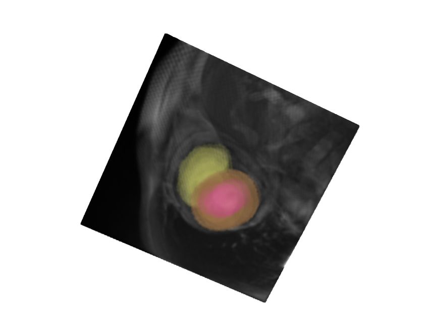
Tomar Vray Thiran Bozorgtabar

Heart Image Segmentation Dataset (M&Ms) (Campello et al., 2021). This dataset
contains 375 studies from six centers and four scanner vendors coded as A, B, C, and D
with three segmentation classes - Left Ventricle, Right Ventricle, and Myocardium.
Prostate MRI Segmentation Dataset (Liu et al., 2020). This dataset is acquired from
six different sites (A, B, C, D, E, F) with various imaging scanners annotated with the
prostate area. Following the protocol of (Liu et al., 2020), we discard site C as it contains
data from unhealthy patients. See Appendix B for more details about three MRI datasets.
Implementation Details: We adopt 2D U-Net architecture (Ronneberger et al., 2015)
instead of the 3D version due to large variance in (volume shape, voxel spacing, and a
number of axial slices from different centers) for the segmentation backbone trained on the
source domain images using a combination of Dice and weighted cross-entropy losses. The
source segmentation network is trained using data augmentation from set O (cf. Section
2.1), RMSprop optimizer with a learning rate of 10−5 (decay factor of 0.1 with 2 epochs
patience), weight decay of 10−4 , and momentum of 0.9 for 250K iterations. We set α1 = 0.01
and α2 = 0.005, respectively (cf. Table 4, Appendix D.2). We also set |texplore | = 1, k = 3,
|Nτ | = 5, M = 128 for the main experiments of Table 1 (cf. Figs. 6, 7, and Table 6,
Appendix D.2), and learning rate of 10−3 , β = (0.9, 0.999), weight decay of 10−4 for OptTTA
Algorithm (Appendix A). All baselines are implemented in PyTorch (Paszke et al., 2019)
and trained on NVIDIA GeForce RTX 3080 GPU. We use Hausdorff Distance (Dubuisson
and Jain, 1994) (cf. Table 8, Appendix D.5.1) and Dice (%) as the evaluation metrics.

3.2. Comparison to State-of-the-Arts
Table 1 shows the quantitative comparison results (Dice (%)) with state-of-the-art methods:
(a) UDA method including ADVENT (Vu et al., 2019) and ProDA (Zhang et al., 2021); (b)
TTMA approaches including TENT (Wang et al., 2021), test-time normalization (BN) (Nado
et al., 2020), where BN layers are updated with test domain statistics, and our new baseline
(PL) that generates pseudo-labels by tuning a confidence threshold to optimize the model;
and (c) TTA methods including greedy policy search (GPS*) (Lyzhov et al., 2020)1 , RandAug
(Cubuk et al., 2020), and Vanilla test-time Augmentation (VA) (random crop, rotation,
and flipping). Overall, OptTTA achieves the most significant average Dice improvement
(9.2%, 22.5%, and 1.7% on Spinal Cord, Heart, and Prostate MRI datasets) compared to
trained Source Model without adaptation. The TTMA baselines alleviate the reliance on
the source domain and adapt to new test image volumes in an online fashion, but they often
make incorrect predictions under substantial domain shifts leading to error accumulation
and performance deterioration (Heart dataset). Similar observations hold for UDA methods
that may encounter the deterioration of feature discriminability despite concurrent access
to source and target samples. TTA methods marginally improve performance due to their
static policies and limited search space. As shown in Fig. 2, OptTTA overcomes the above
shortcomings by learning suitable augmentation policies and magnitudes of transformations
necessary to alleviate domain shift and generate source-like augmented images, thus improving
generalization capability on the test set. More qualitative are provided in Appendix D.5.
Aleatoric Uncertainty and Model Calibration Analysis. We analyze TTA-based
aleatoric uncertainty with the lens of model calibration visualized with a reliability diagram
 1. GPS is adapted for the segmentation task using LOptTTA criterion in Sec. 2.2.1.

                                                    6
Learnable Test-Time Augmentation for Source-Free Medical Image Segmentation

Table 1: Dice (%) results of mean(±std) on three datasets. The largest domain gap w.r.t.
         source domain is highlighted in red, and Bold values denote the best performances.

                             Lower Bound          UDA                            TTMA                                        TTA
  Target              #        Source
                                           ADVENT       ProDA         BN          TENT         PL          VA        RandAug       GPS*       OptTTA
   site            Volumes     Model
  (Source Site 1)                                                                Spinal Cord
            2         10      77.4±6.6     83.0±3.6    86.0±2.2    85.2±2.1      85.7±1.8    85.3±2.1    79.1±4.6    82.7±3.2    81.7±5.0      85.0±2.5
            3         10      64.8±11.7    80.9±3.7    79.7±3.7    70.6±3.6      68.7±2.8    71.0±3.6    66.0±12.9   66.9±12.2   78.4±5.5     82.0±2.7†
            4         10      85.9±3.8     87.4±2.8    89.0±1.5    88.9±1.7      88.9±1.7    88.9±1.7    86.0±2.4    86.9±2.1    87.1±2.9      88.8±1.7
                Average       76.0±11.8    83.8±4.3    84.9±4.7    81.6±8.3      81.1±9.1    81.7±8.6    77.0±11.5   78.8±11.7   82.5±5.9      85.2±3.6
  (Source Sites A,B)                                                                Prostate
            D         13      75.8±8.9     75.2±9.4    83.3±4.8    75.9±9.4      78.8±6.2    76.1±9.4    81.6±6.3    80.1±7.6    77.3±7.7     86.6±4.0†
            E         12      65.9±18.5    63.4±13.4   82.8±6.0    74.4±7.4      77.9±6.9    74.8±7.5    68.1±20.6   66.8±20.7   64.1±27.0     79.8±8.1
            F         12      38.4±32.3    47.6±31.3   63.3±28.7   65.7±22.4     67.0±28.4   66.2±22.4   53.3±33.1   56.6±31.5   57.8±17.2    82.1±8.3
                Average       60.5±27.0    62.4±23.2   76.7±19.3   72.1±15.2     74.7±17.9   72.4±15.2   68.1±25.4   68.3±24.0   66.7±20.5    83.0±7.5†
  (Source Site A)                                                                    Heart
            B        250       87.6±4.2    87.2±4.7    88.3±3.5    85.2±6.0      82.1±7.8    85.3±6.0    87.7±3.5    87.7±3.5    85.9±4.6     88.7±3.6‡
            C        100       85.5±4.4    83.9±5.8    86.4±3.5    82.9±6.3      79.9±7.7    83.0±6.3    87.2±3.6    87.1±3.7    85.6±6.1     87.8±3.4‡
            D        100       86.0±4.0    84.7±4.3    87.4±3.4    83.3±6.6      80.2±7.8    83.4±6.5    88.0±3.9    88.2±3.3    85.5±5.9     88.3±3.9
                Average        86.7±4.5    85.8±5.2    87.5±3.7    84.1±6.6      80.9±8.2    84.2±6.6    87.6±3.8    87.6±3.6    85.5±5.3     88.4±3.6‡
[‡] p < 0.005, [†] 0.005 < p < 0.05: A paired t-test with respect to the top results.

            Target Image                       Evolution of top sub-policy                                                                  Source Site
Spinal
Cord
 Prostate
 Heart

Figure 2: From left to right, starting from the initial augmented test image, we show the
          evolution of the top sub-policy on sample test images per dataset by a fixed step
          size of 110 iterations. The last column shows the corresponding source images.

(Niculescu-Mizil and Caruana, 2005). As shown in Fig. 3, different baselines’ model
performances are plotted against the binned confidence scores. Overall, Fig. 3 shows
several compared baselines fail to output reliable confidence estimates matching the true
underlying model performance when tested on sites other than the source site. Even when
the model is inaccurate, these baselines make high confidence predictions making them
unreliable. In contrast, OptTTA shows significantly better calibration for the segmentation
classes. Our observations are supported with model uncertainty metrics, Brier score, and the
Negative Log-Likelihood (NLL) (Gomariz et al., 2021) (cf. Appendix C) presented in Fig. 3
(b). OptTTA has a significantly lower Brier (p < 0.005) and NLL scores (0.005 < p < 0.05)
than the second best, which correlates with the greater Dice score. As shown in Fig. 4,
OptTTA outputs higher values of confidence map (i.e., lower aleatoric uncertainty) near the

                                                                             7
Tomar Vray Thiran Bozorgtabar

                        (a)                                               (b)

  Figure 3: (a) Reliability diagrams for pixel-wise predictions and (b) Uncertainty metrics–
            Brier and NLL metrics with Dice scores on the Prostate dataset.

              RandAug     VA     OptTTA       RandAug    VA      OptTTA   RandAug             VA                  OptTTA
                                                                                    1.0                                           1.0
Confidence

                                                                                    0.8                                           0.8

                                                                                    0.6                                           0.6

                                                                                    0.4                                           0.4

                                                                                    0.2                                           0.2
Uncertainty

                                                                                    0.0                                           0.0
                                                                                       0.0    0.2     0.4   0.6      0.8   1.0

                                                                                                                                 Ground
                                                                                                                                  Truth
                        Site D                          Site E                               Site F

  Figure 4: Comparison of the segmentation confidence and uncertainty of OptTTA against
            other TTA baselines for the target sites D, E, F on the Prostate dataset.

  boundary of the segmented prostate compared to other TTA baselines for the model trained
  on source sites A, B and tested on target sites D, E, and F (cf. Appendix C.1).

  4. Conclusion and Future Work

 We propose a novel learnable TTA, OptTTA, for medical image segmentation tailored
 for substantial domain shifts as opposed to the previous TTA methods that use static
 augmentation policies. OptTTA offers a privacy-preserving solution, eliminating the need
 for training data or extra model retraining by generating test-time augmented images in
 the source style, enhancing segmentation performances by dynamically selecting optimal
 policies compared to other baselines. Our method surpasses prior-arts by a large margin
 and provides more reliable predictions.
     OptTTA can be further extended to perform self-training based on the pseudo-labels
 generated by our optimized TTA. Together with the release of our implementation, we
 believe this work will inspire further research on model generalization under a significant
 domain shift in clinical practice.

                                                          8
Learnable Test-Time Augmentation for Source-Free Medical Image Segmentation

References
Mina Amiri, Rupert Brooks, Bahareh Behboodi, and Hassan Rivaz. Two-stage ultrasound
 image segmentation using u-net and test time augmentation. International Journal of
 Computer Assisted Radiology and Surgery, 15:981–988, 2020.

Mathilde Bateson, Hoel Kervadec, Jose Dolz, Hervé Lombaert, and Ismail Ben Ayed. Source-
 relaxed domain adaptation for image segmentation. In International Conference on
 Medical Image Computing and Computer-Assisted Intervention, pages 490–499. Springer,
 2020.

Nicholas Bloch, Anant Madabhushi, Henkjan Huisman, John Freymann, Justin Kirby,
  Michael Grauer, Andinet Enquobahrie, Carl Jaffe, Larry Clarke, and Keyvan Farahani.
  Nci-isbi 2013 challenge: automated segmentation of prostate structures. The Cancer
  Imaging Archive, 370:6, 2015.

Behzad Bozorgtabar, Mohammad Saeed Rad, Dwarikanath Mahapatra, and Jean-Philippe
  Thiran. Syndemo: Synergistic deep feature alignment for joint learning of depth and
  ego-motion. In Proceedings of the IEEE/CVF International Conference on Computer
 Vision, pages 4210–4219, 2019.

Vı́ctor M Campello, Polyxeni Gkontra, Cristian Izquierdo, Carlos Martı́n-Isla, Alireza
   Sojoudi, Peter M Full, Klaus Maier-Hein, Yao Zhang, Zhiqiang He, Jun Ma, et al. Multi-
   centre, multi-vendor and multi-disease cardiac segmentation: the m&ms challenge. IEEE
 Transactions on Medical Imaging, 40(12):3543–3554, 2021.

Chaoqi Chen, Weiping Xie, Wenbing Huang, Yu Rong, Xinghao Ding, Yue Huang, Tingyang
 Xu, and Junzhou Huang. Progressive feature alignment for unsupervised domain
  adaptation. In Proceedings of the IEEE/CVF Conference on Computer Vision and
 Pattern Recognition, pages 627–636, 2019a.

Minghao Chen, Hongyang Xue, and Deng Cai. Domain adaptation for semantic segmentation
 with maximum squares loss. In Proceedings of the IEEE/CVF International Conference
 on Computer Vision, pages 2090–2099, 2019b.

Ekin D Cubuk, Barret Zoph, Jonathon Shlens, and Quoc V Le. Randaugment: Practical
  automated data augmentation with a reduced search space. In Proceedings of the
 IEEE/CVF Conference on Computer Vision and Pattern Recognition Workshops, pages
  702–703, 2020.

Ekin Dogus Cubuk, Barret Zoph, Dandelion Mané, Vijay Vasudevan, and Quoc V. Le.
 Autoaugment: Learning augmentation strategies from data. 2019 IEEE/CVF Conference
 on Computer Vision and Pattern Recognition (CVPR), pages 113–123, 2019.

Qi Dou, Daniel Coelho de Castro, Konstantinos Kamnitsas, and Ben Glocker. Domain
  generalization via model-agnostic learning of semantic features. Advances in Neural
  Information Processing Systems, 32, 2019.

                                           9
Tomar Vray Thiran Bozorgtabar

M-P Dubuisson and Anil K Jain. A modified hausdorff distance for object matching. In
 Proceedings of 12th international conference on pattern recognition, volume 1, pages
 566–568. IEEE, 1994.

Tilmann Gneiting and Adrian E Raftery. Strictly proper scoring rules, prediction, and
  estimation. Journal of the American statistical Association, 102(477):359–378, 2007.

Alvaro Gomariz, Tiziano Portenier, César Nombela-Arrieta, and Orcun Goksel. Probabilistic
  spatial analysis in quantitative microscopy with uncertainty-aware cell detection using
  deep bayesian regression of density maps. arXiv preprint arXiv:2102.11865, 2021.

Yufan He, Aaron Carass, Lianrui Zuo, Blake E Dewey, and Jerry L Prince. Self domain
  adapted network. In International Conference on Medical Image Computing and Computer-
 Assisted Intervention, pages 437–446. Springer, 2020.

Dan Hendrycks, Norman Mu, Ekin D. Cubuk, Barret Zoph, Justin Gilmer, and Balaji
 Lakshminarayanan. AugMix: A simple data processing method to improve robustness
 and uncertainty. Proceedings of the International Conference on Learning Representations
 (ICLR), 2020.

Fabian Isensee, Jens Petersen, Andre Klein, David Zimmerer, Paul F Jaeger, Simon Kohl,
  Jakob Wasserthal, Gregor Koehler, Tobias Norajitra, Sebastian Wirkert, et al. nnu-net:
  Self-adapting framework for u-net-based medical image segmentation. arXiv preprint
  arXiv:1809.10486, 2018.

Xiang Jiang, Qicheng Lao, Stan Matwin, and Mohammad Havaei. Implicit class-conditioned
  domain alignment for unsupervised domain adaptation. In International Conference on
  Machine Learning, pages 4816–4827. PMLR, 2020.

Neerav Karani, Ertunc Erdil, Krishna Chaitanya, and Ender Konukoglu. Test-time adaptable
  neural networks for robust medical image segmentation. Medical Image Analysis, 68:
 101907, 2021.

Ildoo Kim, Younghoon Kim, and Sungwoong Kim. Learning loss for test-time augmentation.
   Advances in Neural Information Processing Systems. 33, 2020.

Dong-Hyun Lee et al. Pseudo-label: The simple and efficient semi-supervised learning
 method for deep neural networks. In Workshop on challenges in representation learning,
 ICML, volume 3, page 896, 2013.

Guillaume Lemaı̂tre, Robert Martı́, Jordi Freixenet, Joan C Vilanova, Paul M Walker, and
 Fabrice Meriaudeau. Computer-aided detection and diagnosis for prostate cancer based
 on mono and multi-parametric mri: a review. Computers in biology and medicine, 60:
 8–31, 2015.

Haoliang Li, YuFei Wang, Renjie Wan, Shiqi Wang, Tie-Qiang Li, and Alex Kot. Domain
 generalization for medical imaging classification with linear-dependency regularization.
 Advances in Neural Information Processing Systems, 33:3118–3129, 2020.

                                           10
Learnable Test-Time Augmentation for Source-Free Medical Image Segmentation
Sungbin Lim, Ildoo Kim, Taesup Kim, Chiheon Kim, and Sungwoong Kim. Fast autoaugment.
Advances in Neural Information Processing Systems, 32:6665–6675, 2019.
Geert Litjens, Robert Toth, Wendy van de Ven, Caroline Hoeks, Sjoerd Kerkstra, Bram
van Ginneken, Graham Vincent, Gwenael Guillard, Neil Birbeck, Jindang Zhang, et al.
Evaluation of prostate segmentation algorithms for mri: the promise12 challenge. Medical
image analysis, 18(2):359–373, 2014.
Quande Liu, Qi Dou, Lequan Yu, and Pheng Ann Heng. Ms-net: multi-site network for
improving prostate segmentation with heterogeneous mri data. IEEE transactions on
medical imaging, 39(9):2713–2724, 2020.
Yuang Liu, Wei Zhang, and Jun Wang. Source-free domain adaptation for semantic
segmentation. In Proceedings of the IEEE/CVF Conference on Computer Vision and
Pattern Recognition, pages 1215–1224, 2021.
Ilya Loshchilov and Frank Hutter. Decoupled weight decay regularization. In International
Conference on Learning Representations, 2018.
Alexander Lyzhov, Yuliya Molchanova, Arsenii Ashukha, Dmitry Molchanov, and Dmitry
Vetrov. Greedy policy search: A simple baseline for learnable test-time augmentation. In
Conference on Uncertainty in Artificial Intelligence, pages 1308–1317. PMLR, 2020.
Nikita Moshkov, Botond Mathe, Attila Kertész-Farkas, Réka Hollandi, and Péter Horváth.
Test-time augmentation for deep learning-based cell segmentation on microscopy images.
Scientific Reports, 10, 2020.
Zachary Nado, Shreyas Padhy, D Sculley, Alexander D’Amour, Balaji Lakshminarayanan,
and Jasper Snoek. Evaluating prediction-time batch normalization for robustness under
covariate shift. arXiv preprint arXiv:2006.10963, 2020.
Alexandru Niculescu-Mizil and Rich Caruana. Predicting good probabilities with supervised
learning. In Proceedings of the 22nd international conference on Machine learning, pages
625–632, 2005.
Adam Paszke, Sam Gross, Francisco Massa, Adam Lerer, James Bradbury, Gregory Chanan,
Trevor Killeen, Zeming Lin, Natalia Gimelshein, Luca Antiga, et al. Pytorch: An
imperative style, high-performance deep learning library. Advances in neural information
processing systems, 32:8026–8037, 2019.
Viraj Prabhu, Shivam Khare, Deeksha Kartik, and Judy Hoffman. Sentry: Selective
entropy optimization via committee consistency for unsupervised domain adaptation.
In Proceedings of the IEEE/CVF International Conference on Computer Vision, pages
8558–8567, 2021.
Ferran Prados, John Ashburner, Claudia Blaiotta, Tom Brosch, Julio Carballido-Gamio,
Manuel Jorge Cardoso, Benjamin N Conrad, Esha Datta, Gergely Dávid, Benjamin
De Leener, et al. Spinal cord grey matter segmentation challenge. Neuroimage, 152:
312–329, 2017.
11Tomar Vray Thiran Bozorgtabar
Olaf Ronneberger, Philipp Fischer, and Thomas Brox. U-net: Convolutional networks for
biomedical image segmentation. In International Conference on Medical image computing
and computer-assisted intervention, pages 234–241. Springer, 2015.
Divya Shanmugam, Davis Blalock, Guha Balakrishnan, and John Guttag. Better aggregation
in test-time augmentation. In Proceedings of the IEEE/CVF International Conference on
Computer Vision, pages 1214–1223, 2021.
Yu Sun, Xiaolong Wang, Zhuang Liu, John Miller, Alexei Efros, and Moritz Hardt. Test-time
training with self-supervision for generalization under distribution shifts. In International
Conference on Machine Learning, pages 9229–9248. PMLR, 2020.
Devavrat Tomar, Manana Lortkipanidze, Guillaume Vray, Behzad Bozorgtabar, and Jean-
Philippe Thiran. Self-attentive spatial adaptive normalization for cross-modality domain
adaptation. IEEE Transactions on Medical Imaging, 40(10):2926–2938, 2021a.
Devavrat Tomar, Lin Zhang, Tiziano Portenier, and Orcun Goksel. Content-preserving
unpaired translation from simulated to realistic ultrasound images. In International
Conference on Medical Image Computing and Computer-Assisted Intervention, pages
659–669. Springer, 2021b.
Gabriele Valvano, Andrea Leo, and Sotirios A Tsaftaris. Stop throwing away discriminators!
re-using adversaries for test-time training. In Domain Adaptation and Representation
Transfer, and Affordable Healthcare and AI for Resource Diverse Global Health, pages
68–78. Springer, 2021.
Tuan-Hung Vu, Himalaya Jain, Maxime Bucher, Matthieu Cord, and Patrick Pérez. Advent:
Adversarial entropy minimization for domain adaptation in semantic segmentation. In
Proceedings of the IEEE/CVF Conference on Computer Vision and Pattern Recognition,
pages 2517–2526, 2019.
Dequan Wang, Evan Shelhamer, Shaoteng Liu, Bruno Olshausen, and Trevor Darrell.
Tent: Fully test-time adaptation by entropy minimization. In International
Conference on Learning Representations, 2021. URL https://openreview.net/forum?
id=uXl3bZLkr3c.
Guotai Wang, Wenqi Li, Sébastien Ourselin, and Tom Vercauteren. Automatic brain
tumor segmentation using convolutional neural networks with test-time augmentation. In
International MICCAI Brainlesion Workshop, pages 61–72. Springer, 2018.
Guotai Wang, Wenqi Li, Michael Aertsen, Jan Deprest, Sébastien Ourselin, and Tom
Vercauteren. Aleatoric uncertainty estimation with test-time augmentation for medical
image segmentation with convolutional neural networks. Neurocomputing, 338:34–45, 2019.
Pan Zhang, Bo Zhang, Ting Zhang, Dong Chen, Yong Wang, and Fang Wen. Prototypical
pseudo label denoising and target structure learning for domain adaptive semantic
segmentation. In Proceedings of the IEEE/CVF Conference on Computer Vision and
Pattern Recognition, pages 12414–12424, 2021.
12Learnable Test-Time Augmentation for Source-Free Medical Image Segmentation
Appendix A. Algorithm for OptTTA Optimization
Here we present the algorithm for optimizing a TTA sub-policy. The number of gradient
steps for sub-policy τ is determined by the phase it is being updated. During Exploration,
explore
the gradient steps are kept much greater in Exploration phase (Ngrad ∼ 1000) than in
exploit
Exploitation phase (Ngrad ∼ 100).
Input:
Mode ∈ {explore, exploit}
Trained segmentation model p(y|x) on source data;
Target Image Volume tMode ;
Sub-policy τ (θτ ) : {Onτ (x; λτn ) : n = 1, ..., Nτ };
Gradient Descent Steps Ngrad Mode ; Learning rate η;
Batch size B of 2D augmented images for one iteration;
Output:
Optimized sub-policy τ ∗
Initialization:
for i ∈ {1, ..., Nτ } do
θiτ ← {0, 0.01} /* initialize with small number */
end
Optimization:
Mode do
for j ← 1 to Ngrad
X ← {}
for b ← 1 to B do
a ← U(tMode ) /* sample 2D slice from tMode */
for i ← 1 to Nτ do
λτi ← µτi + σiτ · U(−1, 1) /* re-parametrization trick */
a ← Oiτ (a; λτi ) /* apply augmentations from τ */
end
X ← X ∪ {a}
end
θτ ← θτ − η∇θτ L(X) /* defined in Eq. 8 */
end
return τ (θτ )
A.1. Analysis and Discussion of Computational Complexity
We conduct our experiments using NVIDIA GeForce RTX 3080 (6 optimization steps
per second). Given a set of S sub-policies, the Exploration phase takes approximately
Texplore = 166.67 ∗ |S|, in which a single sub-policy optimization (1000 iterations) takes
around 166.67 seconds. Then, once we obtain the top-k sub-policies from the Exploration
phase, the prediction for each volume takes approximately Texploit = k ∗ 16.67 + M ∗ D ∗ 0.007
seconds, in which M denotes the number of generated augmented views, and D denotes the
depth of the corresponding volume (number of 2D slices). The duration of the Exploitation
phase on one sub-policy (100 iterations) takes 16.67 seconds, and the prediction cost of a
13Tomar Vray Thiran Bozorgtabar
Table 2: The volume-wise computational time (seconds/volume) of OptTTA against several
TTA baselines using NVIDIA GeForce RTX 3080. We report Texploit for OptTTA,
Texplore being negligible as N tends to be large in practice. The times below are
computed on the Spinal Cord (Prados et al., 2017) target site 3, Prostate MRI
dataset (Liu et al., 2020) target site F and Heart dataset (Campello et al., 2021)
target site C, respectively. We report the highest inference time we observed for
each dataset and model.
Method VA RandAug GPS* OptTTA OptTTA (M=2)
Spinal Cord
37.83 39.35 178.21 122.12 64.60
(26 ≤ D ≤ 28)
Prostate
29.99 30.03 158.60 110.12 61.90
(D = 24)
Heart
17.31 17.21 92.85 82.12 53.68
(5 ≤ D ≤ 13)
single 2D slice image takes 0.007 seconds. Thus, the time complexity to process N test
image volumes is 1 ∗ Texplore + (N − 1) ∗ Texploit , where TexploitLearnable Test-Time Augmentation for Source-Free Medical Image Segmentation
label voting to merge these segmentation masks. The range of voxel resolutions varies from
0.25×0.25×2.5 mm to 0.5×0.5×5 mm, and the number of slices per volume ranges from 3 to
20. All the volumes were center cropped in the transverse plane with the crop size of 50mm
and then resized to shape 256 × 256 pixels. The 2D slices in the transverse plane were used
for training the segmentation model and inference. We use images from site 1 as the source
domain while sites 2, 3, 4 are used as the target domain.
B.2. Heart Image Segmentation Dataset (M&Ms) (Campello et al., 2021)
This dataset is composed of 375 patients with hypertrophic, dilated cardiomyopathies, and
healthy subjects collected by six clinical centers from Spain, Canada, and Germany. As the
data from the Canadian clinical center (# 6) is not publicly available, we use 340 patients
in this work. The MRI scans come from four different vendors – A (Siemens) for center # 1,
B (Philips) for center # 2 and 3, C (GE) for center # 4, and D (Canon) for center # 5.
Each patient data is composed of several timestamped 3D volumes, out of which only a few
timestamps (mostly 2) are annotated. In total, we use 190 annotated volumes from vendor
A, 250 annotated volumes from vendor B, and 100 annotated volumes from vendor C and D.
The range of voxel resolutions varies from 0.85×0.85×10 mm to 1.45×1.45×9.9 mm. All
the volumes are first centered cropped to include only the heart region, followed by resizing
the slices in the sagittal plane to 256 × 256 pixels. We use sagittal slices for training the
segmentation model and inference. We use volumes from vendor A as the source domain
and volumes from vendor B, C, D as the target domain.
B.3. Prostate MRI Segmentation Dataset (Liu et al., 2020)
This is a multi-site dataset containing T2-weighted MRI for prostate anatomy with a
segmentation mask collected from six different data sources out of three public datasets.
The samples of site A, B are from NCI-ISBI 2013 dataset (Bloch et al., 2015), samples of
site C are from Initiative for Collaborative Computer Vision Benchmarking (I2CVB) dataset
(Lemaı̂tre et al., 2015), and sites D, E, F are from Prostate MR Image Segmentation 2012
(PROMISE12) dataset (Litjens et al., 2014). Following (Liu et al., 2020), we discard site C
samples as they are mostly from unhealthy patients. Sites A, B, D, E, F contains 30, 30, 13,
12, 12 image volumes respectively. The volumes in this dataset are already centered cropped
along the transverse plane with a size of 384 × 384 pixels used for training the segmentation
model and inference. Sites A, B are used as the source domain, while sites D, E, F are used
as the target domain.
Appendix C. Uncertainty Metrics
The segmentation uncertainty can be evaluated by associating the model output’s confidence
with the correctness of the model predictions at the pixel level. Generally, strictly proper
scoring rules are used to assess the calibration quality of predictive models (Gneiting and
Raftery, 2007). We use three such metrics – Expected Calibration Error, Brier score and
NLL (Gomariz et al., 2021). Table 3 provides the uncertainty measures of several methods
computed on the Prostate dataset.
15Tomar Vray Thiran Bozorgtabar
Table 3: Uncertainty analysis on the Prostate dataset.
Method ECE Br NLL
Source Model 17.37 0.265 1.188
TENT 8.27 0.172 0.675
RandAug 9.60 0.204 0.723
OptTTA 3.49 0.139 0.528
Expected Calibration Error (ECE) (lower is better). The Expected Calibration
Error analyzes the confidence values of test images predicted by the model versus their
measured expected accuracy values. It measures whether the model is overconfident (high
confidence and low accuracy) or under-confident (low confidence and high accuracy). For
calculating the expected accuracy measurement, the pixels are put into M bins according to
their confidences predicted by the model, and the accuracy for each bin is computed. ECE
is then calculated by summing up the weighted average of the differences between accuracy
and the average confidence over the bins as follows:
M
X Nm
ECE = · |Acc(m) − Conf (m)| (10)
N
m=1
where Nm is the number of pixels, Acc(m) is the average accuracy of pixels, Conf (m) is
the confidence of the mth bin, and N is the total number of pixels.
Brier score (Br) (lower is better). The Brier score is a strictly proper score function
that measures the accuracy of probabilistic predictions. It is equivalent to the mean squared
error of the predicted probabilities with respect to ground truth. For a collection of C
possible segmentation classes, and N pixels, Br metric can be computed as:
N C
1 X 1 X
Br = [p(yˆi = yc |xi ) − (yˆi = yc )]2 (11)
N C
i=1 c=1
NLL (lower is better). This metric measures the joint probability of observed data and
can be used to estimate the uncertainty of the model predictions.
N C
1 XX
N LL = − ln(p(yˆi = yc |xi )) · (yˆi = yc ) (12)
N
i=1 c=1
where p(yˆi = yc |xi ) is the output confidence of the model for the class yc and input xi .
C.1. Aleatoric Uncertainty
We evaluate OptTTA in terms of aleatoric uncertainty estimation (Wang et al., 2019). This
experiment shows that learning an optimal TTA policy by OptTTA further refines aleatoric
uncertainty estimation than other TTA baselines like VA and RandAug. In particular, the
dashed ellipses in Fig. 5 show that OptTTA leads to a lower error rate (occurrence) of
overconfident incorrect predictions than other TTA baselines. Moreover, our joint histogram
16Learnable Test-Time Augmentation for Source-Free Medical Image Segmentation
0.01 0.1 1
1.0
0.8
Error rate
0.5
0.2
0.0
0.00 0.09 0.17 0.26 0.35 0.00 0.09 0.17 0.26 0.35 0.00 0.09 0.17 0.26 0.35
Uncertainty Uncertainty Uncertainty
VA RandAug OptTTA
Figure 5: Normalized joint histogram of uncertainty estimation and error rate on the Prostate
dataset. Given a pixel-wise uncertainty level (x-axis), we associate the frequency
of pixel error rates along with the slices (y-axis). The red curve represents the
mean error rate per uncertainty bin and dashed ellipses highlight the frequency of
high error rates on different levels of overconfident predictions from VA, RandAug,
and OptTTA.
is less noisy and shows an apparent monotonic increase of the error rate with respect to the
uncertainty. These observations witness the efficiency of our learnable TTA policy framework
in estimating the uncertainty under a domain shift scenario.
Appendix D. Ablations
In this section, we present several ablation studies for the proposed method OptTTA on the
Prostate dataset concerning sub-policy optimization criterion LOptTTA , effects of exploration
and exploitation, and test time performance based on the source model training strategy.
D.1. Ablation Study on the Hyper-parameters of Loss Terms
We provide a sensitivity test of the hyper-parameters of the optimization criterion of OptTTA
on the segmentation accuracy. Table 4 shows the effect of changing hyper-parameters of
individual loss terms of LOptTTA by order of magnitude 10. We observe that the final
segmentation accuracy is slightly sensitive to α2 . It demonstrates that Entropy of Class
Marginal (Lcm ) is an important loss term for improving accuracy without supervision.
However, it forces uniform prediction and degrades performance as its value increases. On
the other hand, the segmentation accuracy is not very sensitive to α1 on average. We observe
that penalizing the BN statistics discrepancy helps the Spinal Cord and Heart Datasets but
slightly harms the Prostate dataset. This implies that our method can be applied to model
architectures without BN layers.
D.2. Exploration vs. Exploitation
In this subsection, we conduct several ablation experiments on the Exploration and Exploitation
phases of OptTTA to justify the choice of sub-policy selection criterion, size of a sub-policy,
and number of target domain images necessary for exploration.
17Tomar Vray Thiran Bozorgtabar
Table 4: Sensitivity test with respect to hyper-parameters of LOptTTA .
Hyperparameters Dice (%)
α1 α2 Spinal Cord Prostate Heart Average
0.01 0.005 85.2±3.6 83.0±7.5 88.4±3.6 85.5
0 84.1±4.8 83.5 ±7.2 87.9±4.5 85.2
0.001 0.005 84.3±3.9 83.5 ±8.6 88.0±4.5 85.3
0.1 84.8±4.1 81.0±9.6 87.9±4.5 84.6
0 85.3±3.8 80.5±11.4 88.0±3.4 84.6
0.01 0.0005 85.3±3.8 80.9±10.5 88.3±3.4 84.8
0.05 81.7±5.3 78.1±9.6 86.4±6.1 82.1
(a) (b)
83.6 p = 0.90 *
82
83.4
80
83.2
78
Dice Score (%)
Dice Score (%)
83.0
76
82.8
74
82.6
72
82.4
70
82.2
68
82.0
1 2 3 4 5 1/N % 25% 50% 75%
|N | |texplore |
[∗ ]Paired t-test with respect to the top result.
Figure 6: (a) Dice (%) vs. |Nτ | on the Prostate dataset. (b) Dice (%) vs. |texplore | on the
Prostate dataset. N is the size of the target site.
Ablation on Selecting Top-k Sub-Policies. The last and crucial step of the Exploration
phase is selecting the sub-set T ∗ comprising the top-k sub-policies from the set of optimized
sub-policies S ∗ . Table 5 shows the segmentation accuracy when different loss terms are
used as the selection metric for the top-k sub-policies. We observe that LOptTTA is the best
choice for selection.
Ablation on the Number of Augmentations Used in a Sub-Policy. Fig. 6 (a) shows
the effect of changing the maximum size Nτ of sub-policy τ . We observe that concatenating
various augmentation operations helps in generating source-like augmented images and
higher segmentation accuracy.
Ablation on the Number of top-k Sub-Policies in the Exploitation Phase. Table
6 shows the effect of changing the number of top-k policies on the Spinal Cord dataset for
sites 1 to 3. We observe that including all sub-policies degrades performance.
18Learnable Test-Time Augmentation for Source-Free Medical Image Segmentation
Table 5: Effect of changing sub-policy selection metric on the Prostate dataset. Using
LOptT T A or Lbn leads to similar performance while using Lent alone degrades
performance.
Selection Metric LOptTTA Lbn Lent
Dice (%) 83.0±7.5 82.7±7.6 63.3±25.6
Table 6: Ablation experiment on the number of Top-k sub-policies in the Exploitation phase
on the Spinal Cord dataset, with the source site=1 and target site=3.
k 1 2 3 5 10 15 21
Dice (%) 81.1±3.4 81.3±3.2 82.0±2.7 80.9±4.6 81.4±4.0 81.6±3.4 80.1±5.4
Ablation on the Number of Augmented Views (M ). As shown in Fig. 7, increasing
the number of augmented views leads to higher prediction accuracy for VA and RandAug.
We observe that we reach a plateau at M = 32. On the other hand, OptTTA seems less
sensitive to values of M , having a similar performance by generating 128 or only two views.
These observations support learning an optimal augmentation policy by TTA methods.
Ablation Study on the Number of Images used for Exploration (|texplore |). In
practice, we do not have access to all test time data at once. However, we can fine-tune
the optimal sub-policies found in the exploration phase on the test images in an online
manner. Since exploration is expensive to compute for every test image, we benefit by
directly applying the optimal sub-policies found during the exploration phase, thus making
inference faster. Fig. 6 (b) shows the effect of exploring more than one target image on the
overall Dice score for the Prostate dataset for sites A, B to F.
D.3. Performance Comparison of TTA Methods Under Different Training
Strategies of the Source Model
The performance of TTA methods often relies on the initial source model performance,
considering these methods’ limitations. Fig. 8 shows correlational analysis supporting that
the accuracy of TTA methods depends on the augmentation policy used for training as well
as the training dataset size. Nevertheless, OptTTA still surpasses the baselines on these
particular settings showing our method is more robust under these training setup variations.
D.4. Performance Comparison of Baselines Using Multiple Source Domains
We also show the quantitative comparison results (Dice (%)) with state-of-the-art methods
on the Spinal Cord dataset and trained on multiple source domains. Overall, aggregating
information from diverse source domains can improve the model’s generalization capability
compared to the models trained on a single source only. As shown in Table 7, OptTTA
19Tomar Vray Thiran Bozorgtabar
85.0
82.5
80.0 M
2
Dice Score (%)
77.5
4
75.0 8
16
72.5 32
70.0 64
128
67.5 256
65.0
OptTTA VA RandAug
Method
Figure 7: Dice (%) scores vs. M values on the Prostate dataset for various TTA methods,
including OptTTA, VA, and RandAug.
80
60
Dice Score (%)
Dice Score (%)
40
20 Method
Source Model
OptTTA
Tent
0 RandAug
25 50 100 RandAug VA w/o
Training dataset size (%) Training Augmentation
Figure 8: Correlation analysis of the Dice (%) scores vs. training data size and training
augmentation policy on the Prostate dataset.
20Learnable Test-Time Augmentation for Source-Free Medical Image Segmentation
Table 7: Dice (%) results of mean(±std) on the Spinal Cord dataset. The models are trained
on multiple source domains. The largest domain gap w.r.t. source domain is
highlighted in red, and Bold values denote the best performances.
Lower bound UDA TTMA TTA
Source Target
DeepAll ADVENT ProDA BN TENT PL VA RandAug GPS* OptTTA
site(s) site(s)
2,3,4 1 88.0±2.7 86.0±4.3 87.7±2.9 86.3±3.2 86.7±3.2 86.4±3.1 86.5±3.0 85.8±3.3 85.6±3.2 87.3±2.2
1,3,4 2 88.3±0.7 87.6±0.9 87.9±0.8 87.2±0.9 87.2±0.7 87.1±0.8 87.3±0.9 87.3±0.9 87.8±0.8 88.1±0.6
1,2,4 3 50.5±28.3 85.8±1.8 78.2±2.5 69.5±5.6 74.4±2.3 71.9±5.0 48.3±28.5 45.6±27.2 70.0±16.7 87.0±2.0‡
1,2,3 4 90.9±1.1 88.5±2.3 90.8±1.0 90.5±1.2 90.3±1.3 90.4±1.2 90.0±0.9 89.7±0.9 89.8±1.2 90.0±0.8
Average 79.4±21.9 87.0±2.9 86.1±5.2 83.4±8.8 84.7±6.4 84.0±7.7 78.0±22.4 77.1 ±22.8 83.3±12.5 88.1±2.0‡
[‡] p < 0.005, [†] 0.005 < p < 0.05: A paired t-test with respect to the top results.
significantly outperforms other TTA methods on average and shows marginal gains over state-
of-the-art UDA methods while not using information about source domains. Additionally,
we provide a new baseline, DeepAll, by aggregating all source domains data followed by
segmentation model standard training. OptTTA achieves competitive performance on par
with DeepAll in most cases without using knowledge from source domains. Nevertheless,
in the presence of substantial domain shift (target site=3), OptTTA significantly improves
the accuracy upon DeepALL, demonstrating our model’s generalization aspects under large
domain shift.
D.5. Additional Results
D.5.1. Hausdorff Distance Metric and Qualitative Results
Table 8 compares the Harmonic Mean 95th percentile Hausdorff Distance (HD95) of the
segmentation predicted by OptTTA against several baselines, while Fig. 9 and Fig. 10 show
additional qualitative segmentation results on 2D slices and 3D volumes, respectively.
D.5.2. Evolution of Sub-Policies in Exploration and Exploitation Phases
Exploration Phase. Fig. 11 shows the evolution of 21 different sub-policies on a sample
test image from the Spinal Cord dataset by a fixed step size of 80 iterations. We observe
that the segmentation prediction of the source model on the target image improves as
the parameters of a sub-policy are optimized using the loss LOptTTA defined in Sec. 2.2.1.
However, not all the sub-policies perform equally well at the end of optimization.
Exploitation Phase. Fig. 12 shows segmentation results on augmented views of the
target image obtained by fine-tuning top-3 sub-policies T ∗ found in the Exploration phase.
21Tomar Vray Thiran Bozorgtabar
Source
GT Model ADVENT ProDA BN TENT PL VA RandAug GPS* OptTTA
Spinal Cord
Prostate
Heart
Figure 9: Qualitative segmentation results (2D slices) on three multi-center, multi-vendor
MRI datasets: Spinal Cord (Prados et al., 2017), Prostate (Liu et al., 2020) and
Heart dataset (Campello et al., 2021).
22Learnable Test-Time Augmentation for Source-Free Medical Image Segmentation
Volume Ground Truth Source Model TENT RandAug OptTTA
Site 2
Spinal
Cord
Site 3
Site 4
Site D
Prostate
Site E
Site F
Site B
Heart
Site C
Site D
Figure 10: Qualitative 3D segmentation results on three multi-center, multi-vendor MRI
datasets: Spinal Cord (Prados et al., 2017), Prostate (Liu et al., 2020) and Heart
dataset (Campello et al., 2021).
23Tomar Vray Thiran Bozorgtabar
Number of iterations
Sub-policies
1
2
3
4
5
6
7
8
9
10
11
12
13
14
15
16
17
18
19
20
21
Figure 11: Evolution of 21 sub-policies during the Exploration phase on the Spinal Cord
dataset.
24Learnable Test-Time Augmentation for Source-Free Medical Image Segmentation
Target Image Top-1 sub-policy Top-2 sub-policy Top-3 sub-policy
Figure 12: Exploiting top-3 sub-policies after the Exploration phase on the Spinal Cord
dataset. The first column shows the segmentation prediction of the source model
directly on the target image. The next three columns show the augmented
views of the target image generated by the top-1, top-2 and top-3 policies in
the Exploitation phase and their corresponding segmentations predicted by the
source model.
25You can also read