PDE-DRIVEN SPATIOTEMPORAL DISENTANGLEMENT
←
→
Page content transcription
If your browser does not render page correctly, please read the page content below
Published as a conference paper at ICLR 2021

PDE-D RIVEN S PATIOTEMPORAL D ISENTANGLEMENT
 Jérémie Donà,†∗ Jean-Yves Franceschi,†∗ Sylvain Lamprier† & Patrick Gallinari†‡
 †
   Sorbonne Université, CNRS, LIP6, F-75005 Paris, France
 ‡
   Criteo AI Lab, Paris, France
 firstname.lastname@lip6.fr

                                                  A BSTRACT

              A recent line of work in the machine learning community addresses the problem
              of predicting high-dimensional spatiotemporal phenomena by leveraging specific
              tools from the differential equations theory. Following this direction, we propose in
              this article a novel and general paradigm for this task based on a resolution method
              for partial differential equations: the separation of variables. This inspiration allows
              us to introduce a dynamical interpretation of spatiotemporal disentanglement. It
              induces a principled model based on learning disentangled spatial and temporal
              representations of a phenomenon to accurately predict future observations. We
              experimentally demonstrate the performance and broad applicability of our method
              against prior state-of-the-art models on physical and synthetic video datasets.

1        I NTRODUCTION

The interest of the machine learning community in physical phenomena has substantially grown for the
last few years (Shi et al., 2015; Long et al., 2018; Greydanus et al., 2019). In particular, an increasing
amount of works studies the challenging problem of modeling the evolution of dynamical systems,
with applications in sensible domains like climate or health science, making the understanding of
physical phenomena a key challenge in machine learning. To this end, the community has successfully
leveraged the formalism of dynamical systems and their associated differential formulation as
powerful tools to specifically design efficient prediction models. In this work, we aim at studying this
prediction problem with a principled and general approach, through the prism of Partial Differential
Equations (PDEs), with a focus on learning spatiotemporal disentangled representations.
Prediction via spatiotemporal disentanglement was first studied in video prediction works, in order to
separate static and dynamic information (Denton & Birodkar, 2017) for prediction and interpretability
purposes. Existing models are particularly complex, involving either adversarial losses or variational
inference. Furthermore, their reliance on Recurrent Neural Networks (RNNs) hinders their ability
to model spatiotemporal phenomena (Yıldız et al., 2019; Ayed et al., 2020; Franceschi et al., 2020).
Our proposition addresses these shortcomings with a simplified and improved model by grounding
spatiotemporal disentanglement in the PDE formalism.
Spatiotemporal phenomena obey physical laws such as the conservation of energy, that lead to describe
the evolution of the system through PDEs. Practical examples include the conservation of energy for
physical systems (Hamilton, 1835), or the equation describing constant illumination in a scene (Horn
& Schunck, 1981) for videos that has had a longstanding impact in computer vision with optical flow
methods (Dosovitskiy et al., 2015; Finn et al., 2016). We propose to model the evolution of partially
observed spatiotemporal phenomena with unknown dynamics by leveraging a formal method for the
analytical resolution of PDEs: the functional separation of variables (Miller, 1988). Our framework
formulates spatiotemporal disentanglement for prediction as learning a separable solution, where
spatial and dynamic information are represented in separate variables. Besides offering a novel
interpretation of spatiotemporal disentanglement, it confers simplicity and performance compared to
existing methods: disentanglement is achieved through the sole combination of a prediction objective
and regularization penalties, and the temporal dynamics is defined by a learned Ordinary Differential
Equation (ODE). We experimentally demonstrate the applicability, disentanglement capacity and
     ∗
         Equal contribution.

                                                         1
Published as a conference paper at ICLR 2021

forecasting performance of the proposed model on various spatiotemporal phenomena involving
standard physical processes and synthetic video datasets against prior state-of-the-art models.

2     R ELATED W ORK
Our contribution deals with two main directions of research: spatiotemporal disentanglement and the
coupling of neural networks and PDEs.

Spatiotemporal disentanglement. Disentangling factors of variations is an essential representation
learning problem (Bengio et al., 2013). Its cardinal formulation for static data has been extensively
studied, with state-of-the-art solutions (Locatello et al., 2019) being essentially based on Variational
Autoencoders (VAEs; Kingma & Welling, 2014; Rezende et al., 2014). As for sequential data, several
disentanglement notions have been formulated, ranging from distinguishing objects in a video (Hsieh
et al., 2018; van Steenkiste et al., 2018) to separating and modeling multi-scale dynamics (Hsu et al.,
2017; Yingzhen & Mandt, 2018).
We focus in this work on the dissociation of the dynamics and visual aspects for spatiotemporal data.
Even in this case, dissociation can take multiple forms. Examples in the video generation community
include decoupling the foreground and background (Vondrick et al., 2016), constructing structured
frame representations (Villegas et al., 2017b; Minderer et al., 2019; Liu et al., 2019), extracting
physical dynamics (Le Guen & Thome, 2020), or latent modeling of dynamics in a state-space
manner (Fraccaro et al., 2017; Franceschi et al., 2020). Closer to our work, Denton & Birodkar
(2017), Villegas et al. (2017a) and Hsieh et al. (2018) introduced in their video prediction models
explicit latent disentanglement of static and dynamic information obtained using adversarial losses
(Goodfellow et al., 2014) or VAEs. Disentanglement has also been introduced in more restrictive
models relying on data-specific assumptions (Kosiorek et al., 2018; Jaques et al., 2020), and in video
generation (Tulyakov et al., 2018). We aim in this work at grounding and improving spatiotemporal
disentanglement with more adapted inductive biases by introducing a paradigm leveraging the
functional separation of variables resolution method for PDEs.

Spatiotemporal prediction and PDE-based neural network models. An increasing number of
works combining neural networks and differential equations for spatiotemporal forecasting have been
produced for the last few years. Some of them show substantial improvements for the prediction of
dynamical systems or videos compared to standard RNNs by defining the dynamics using learned
ODEs (Rubanova et al., 2019; Yıldız et al., 2019; Ayed et al., 2020; Le Guen & Thome, 2020),
following Chen et al. (2018), or adapting them to stochastic data (Ryder et al., 2018; Li et al.,
2020; Franceschi et al., 2020). Most PDE-based spatiotemporal models exploit some prior physical
knowledge. It can induce the structure of the prediction function (Brunton et al., 2016; de Avila
Belbute-Peres et al., 2018) or specific cost functions, thereby improving model performances. For
instance, de Bézenac et al. (2018) shape their prediction function with an advection-diffusion
mechanism, and Long et al. (2018; 2019) estimate PDEs and their solutions by learning convolutional
filters proven to approximate differential operators. Greydanus et al. (2019), Chen et al. (2020) and
Toth et al. (2020) introduce non-regression losses by taking advantage of Hamiltonian mechanics
(Hamilton, 1835), while Tompson et al. (2017) and Raissi et al. (2020) combine physically inspired
constraints and structural priors for fluid dynamic prediction. Our work deepens this literature by
establishing a novel link between a resolution method for PDEs and spatiotemporal disentanglement,
thereby introducing a data-agnostic model leveraging any static information in observed phenomena.

3     BACKGROUND : S EPARATION OF VARIABLES
Solving high-dimensional PDEs is a difficult analytical and numerical problem (Bungartz & Griebel,
2004). Variable separation aims at simplifying it by decomposing the solution, e.g., as a simple
combination of lower-dimensional functions, thus reducing the PDE to simpler differential equations.

3.1   S IMPLE C ASE S TUDY

Let us introduce this technique through a standard application, with proofs in Appendix A.1, on
the one-dimensional heat diffusion problem (Fourier, 1822), consisting in a bar of length L, whose

                                                   2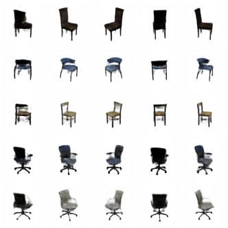
Published as a conference paper at ICLR 2021

temperature at time t and position x is denoted by u(x, t) and satisfies:
             ∂u       ∂2u
                 = c2 2 ,               u(0, t) = u(L, t) = 0,            u(x, 0) = f (x).           (1)
             ∂t       ∂x
Suppose that a solution u is product-separable, i.e., it can be decomposed as: u(x, t) = u1 (x) · u2 (t).
Combined with Equation (1), it leads to c2 u001 (x)/u1 (x) = u02 (t)/u2 (t). The left- and right-hand
sides of this equation are respectively independent from t and x. Therefore, both sides are constant,
and solving both resulting ODEs gives solutions of the form, with µ ∈ R and n ∈ N:
                                                                     2
                           u(x, t) = µ sin nπx/L × exp − cnπ/L t .                                   (2)
The superposition principle and the uniqueness of solutions under smoothness constraints allow then
to build the set of solutions of Equation (1) with linear combinations of separable solutions (Le Dret
& Lucquin, 2016). Besides this simple example, separation of variables can be more elaborate.

3.2   F UNCTIONAL S EPARATION OF VARIABLES

The functional separation of variables (Miller, 1988) generalizes this method. Let u be a function
obeying a given arbitrary PDE. The functional variable separation method amounts to finding a
parameterization z, a functional U , an entangling function ξ, and representations φ and ψ such that:

                     z = ξ φ(x), ψ(t) ,                         u(x, t) = U (z).                 (3)
Trivial choices ξ = u and identity function as U , φ and ψ ensure the validity of this reformulation.
Finding suitable φ, ψ, U , and ξ with regards to the initial PDE can facilitate its resolution by inducing
separate simpler PDEs on φ, ψ, and U . For instance, product-separability is retrieved with U = exp.
General results on the existence of separable solutions have been proven (Miller, 1983), though their
uniqueness depends on the initial conditions and the choice of functional separation (Polyanin, 2020).
Functional separation of variables finds broad applications. It helps to solve refinements of the
heat equation, such as generalizations with an advection term (see Appendix A.2) or with complex
diffusion and source terms forming a general transport equation (Jia et al., 2008). Besides the heat
equation, functional separation of PDEs is also applicable in various physics fields like reaction-
diffusion with non-linear sources or convection-diffusion phenomena (Polyanin, 2019; Polyanin &
Zhurov, 2020), Hamiltonian physics (Benenti, 1997), or even general relativity (Kalnins et al., 1992).
Reparameterizations such as Equation (3) implement a separation of spatial and temporal factors of
variations, i.e., spatiotemporal disentanglement. We introduce in the following a learning framework
based on this general method.

4     P ROPOSED M ETHOD
We propose to model spatiotemporal phenomena using the functional variable separation formalism.
We first describe our notations and then derive a principled model and constraints from this method.

4.1   P ROBLEM F ORMULATION T HROUGH S EPARATION OF VARIABLES

We consider a distribution P of observed spatiotemporal trajectories and corresponding observation
samples v = (vt0 , vt0 +∆t , . . . , vt1 ), with vt ∈ V ⊆ Rm and t1 = t0 + ν∆t. Each sequence v ∼ P
corresponds to an observation of a dynamical phenomenon, assumed to be described by a hidden
functional uv (also denoted by u for the sake of simplicity) of space coordinates x ∈ X ⊆ Rs
and time t ∈ R that characterizes the trajectories. More precisely, uv describes an unobserved
continuous dynamics and v corresponds to instantaneous discrete spatial measurements associated
to this dynamics. Therefore, we consider that vt results from a time-independent function ζ of the
mapping uv (·, t). For example, v might consist in temperatures measured at some points of the sea
surface, while uv would be the complete ocean circulation model. In other words, v provides a partial
information about uv and is a projection of the full dynamics. We seek to learn a model which, when
conditioned on prior observations, can predict future observations.
To this end, we posit that the state u of each observed trajectory v is driven by a hidden PDE, shared
among all trajectories; we discuss this assumption in details in Appendix C.1. Learning such a PDE

                                                    3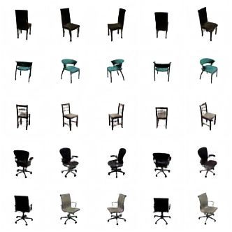
Published as a conference paper at ICLR 2021

Figure 1: Computational graph of the proposed model. ES and ET take contiguous observations
as input; time invariance is enforced on S; the evolution of Tt is modeled with an ODE and is
constrained to coincide with ET ; Tt0 is regularized; forecasting amounts to decoding from S and Tt .

and its solutions would then allow us to model observed trajectories v. However, directly learning
solutions to high-dimensional unknown PDEs is a complex task (Bungartz & Griebel, 2004; Sirignano
& Spiliopoulos, 2018). We aim in this work at simplifying this resolution. We propose to do so by
relying on the functional separation of variables of Equation (3), in order to leverage a potential
separability of the hidden PDE. Therefore, analogously to Equation (3), we propose to formulate the
problem as learning observation-constrained φ, ψ and U , as well as ξ and ζ, such that:

             z = ξ φ(x), ψ(t) ,             u(x, t) = U (z),            vt = ζ u(·, t) ,        (4)
with φ and ψ allowing to disentangle the prediction problem. In the formalism of the functional
separation of variables, this amounts to decomposing the full solution u, thereby learning a spatial
PDE on φ, a temporal ODE on ψ, and a PDE on U , as well as their respective solutions.

4.2   F UNDAMENTAL L IMITS AND R ELAXATION

Directly learning u is, however, a restrictive choice. Indeed, when formulating PDEs such as in
Equation (1), spatial coordinates (x, y, etc.) and time t appear as variables of the solution. Yet, unlike
in fully observable phenomena studied by Sirignano & Spiliopoulos (2018) and Raissi (2018), directly
accessing theses variables in practice can be costly or infeasible in our partially observed setting. In
other words, the nature and number of these variables are unknown. For example, the dynamic of
the observed sea surface temperature is highly dependent on numerous unobserved variables such
as temperature at deeper levels or wind intensity. Explicitly taking into account these unobserved
variables can only be done with prior domain knowledge. To maintain the generality of the proposed
approach, we choose not to make any data-specific assumption on these unknown variables.
We overcome these issues by eliminating the explicit modeling of spatial coordinates by learning
dynamic and time-invariant representations accounting respectively for the time-dependent and space-
dependent parts of the solution. Indeed, Equation (4) induces that these spatial coordinates, hence the
explicit resolution of PDEs on u or U , can be ignored, as it amounts to learning φ, ψ and D such that:

                             vt = (ζ ◦ U ◦ ξ) φ(·), ψ(t) = D φ, ψ(t) .                              (5)
In order to manipulate functionals φ and ψ in practice, we respectively introduce learnable time-
invariant and time-dependent representations of φ and ψ, denoted by S and T , such that:
                  φ ≡ S ∈ S ⊆ Rd ,                     ψ ≡ T : t 7→ Tt ∈ T ⊆ Rp ,                 (6)
where the dependence of ψ ≡ T on time t will be modeled using a temporal ODE following the
separation of variables, and the function φ, and consequently its spatial PDE, are encoded into a
vectorial representation S. Besides their separation of variables basis, the purpose of S and T is to
capture spatial and motion information of the data. For instance, S could encode static information
such as objects appearance, while T typically contains motion variables.
S and Tt0 , because of their dependence on v in Equations (5) and (6), are inferred from an observation
history, or conditioning frames, Vτ (t0 ), where Vτ (t) = (vt , vt+∆t , . . . , vt+τ ∆t ), using respectively
encoder networks ES and ET . We parameterize D of Equation (5) as a neural network that acts on
both S and Tt , and outputs the estimated observation vbt = D(S, Tt ). Unless specified otherwise, S
and Tt are fed concatenated into D, which then learns the parameterization ξ of their combination.

                                                     4
Published as a conference paper at ICLR 2021
4.3 T EMPORAL ODE
The separation of variables allows us to partly reduce the complex task of learning and integrating
PDEs to learning and integrating an ODE on ψ, which has been extensively studied in the literature,
as explained in Section 2. We therefore model the evolution of Tt , thereby the dynamics of our
system, with a first-order ODE:
Z t
∂ Tt
= f (Tt ) ⇔ Tt = Tt0 + f (Tt0 ) dt0 (7)
∂t t0
Note that the first-order ODE assumption can be taken without loss of generality since any ODE is
equivalent to a higher-dimensional first-order ODE. Following Chen et al. (2018), f is implemented
by a neural network and Equation (7) is solved with an ODE resolution scheme. Suppose initial
ODE conditions S and Tt0 have been computed with ES and ET . This leads to the following simple
forecasting scheme, enforced by the corresponding regression loss:
Z t ! ν
0 1 X 1 2
vbt = D S, Tt0 + f (Tt0 ) dt , Lpred = kb
vt +i∆t − vt0 +i∆t k2 , (8)
t0 ν + 1 i=0 m 0
where ν + 1 is the number of observations, and m is the dimension of the observed variables v.
Equation (8) ensures that the evolution of T is coherent with the observations; we should enforce its
consistency with ET . Indeed, the dynamics of Tt is modeled by Equation (7), while only its initial
condition Tt0 is computed
with ET . However, there is no guaranty that Tt , computed via integration,
matches ET Vτ (t) at any other time t, while they should in principle coincide. We introduce the
following autoencoding constraint mitigating their divergence, thereby stabilizing the evolution of T :
2
1
LAE = D S, ET Vτ (t0 + i∆t) − vt0 +i∆t , with i ∼ U J0, ν − τ K . (9)
m 2
4.4 S PATIOTEMPORAL D ISENTANGLEMENT
As indicated hereinabove, the spatial PDE on φ is assumed to be encoded into S. Nonetheless, since
S is inferred from an observation history, we need to explicitly enforce its time independence. In the
PDE formalism, this is equivalent to:
Z t1 −τ ∆t 2
∂ ES Vτ (t) ∂ ES Vτ (t)
=0 ⇔ dt = 0. (10)
∂t t0 ∂t
2
However, enforcing Equation (10) raises two crucial issues. Firstly, in our partially observed setting,
there can be variations of observable content, for instance when an object conceals another one.
Therefore, strictly enforcing a null time derivative is not desirable as it prevents ES to extract
accessible information that could be obfuscated in the sequence. Secondly, estimating this derivative
in practice in our setting is unfeasible and costly because of the coarse temporal discretization of the
data and the computational cost of ES ; see Appendix B for more details. We instead introduce a
discretized penalty in our minimization objective, discouraging variations of content between two
distant time steps, with d being the dimension of S:
1 2
LSreg =
ES Vτ (t0 ) − ES Vτ (t1 − τ ∆t) . (11)
d 2
It allows us to overcome the previously stated issues by not enforcing a strict invariance of S and
removing the need to estimate any time derivative. Note that this formulation actually originates from
Equation (10) using the Cauchy-Schwarz inequality (see Appendix B for a more general derivation).
Abstracting the spatial ODE on φ from Equation (4) into a generic representation S leads, without
additional constraints, to an underconstrained problem where spatiotemporal disentanglement cannot
be guaranteed. Indeed, ES can be set to zero to satisfy Equation (11) without breaking any prior
constraint, because static information is not prevented to be encoded into T . Accordingly, information
in S and T needs to be segmented.
Thanks to the design of our model, it suffices to ensure that S and T are disentangled at initial time
t0 for them be to be disentangled at all t. Indeed, the mutual information between two variables
5Published as a conference paper at ICLR 2021
is preserved by invertible transformations. Equation (7) is an ODE and f , as a neural network, is
Lipschitz-continuous, so the ODE flow Tt 7→ Tt0 is invertible. Therefore, disentanglement between
S and Tt , characterized by a low mutual information between both variables, is preserved through
time; see Appendix C for a detailed discussion. We thus only constrain the information quantity in
Tt0 by using a Gaussian prior to encourage it to exclusively contain necessary dynamic information:
1 1 2
2
LTreg =
kTt0 k2 = ET Vτ (t0 ) . (12)
p p 2
4.5 L OSS F UNCTION
The minimized loss is a linear combination of Equations (8), (9), (11) and (12):
h i
L(v) = Ev∼P λpred Lpred + λAE · LAE + λSreg · LSreg + λTreg · LTreg , (13)
as illustrated in Figure 1. In the following, we conventionally set ∆t = 1. Note that the presented
approach could be generalized to irregularly sampled observation times thanks to the dedicated
literature (Rubanova et al., 2019), but this is out of the scope of this paper.
5 E XPERIMENTS
We study in this section the experimental results of our t=0 t=4 t=6 t=8
model on various spatiotemporal phenomena with phys-
frames
Input
Truth
ical, synthetic video and real-world datasets, which are
briefly presented in this section and in more details in
Appendix D. We demonstrate the relevance of our model
PKnl
with ablation studies and its performance by comparing
it with more complex state-of-the-art models. Perfor-
mances are assessed thanks to standard metrics (Den- PhyDNet
ton & Fergus, 2018; Le Guen & Thome, 2020) Mean
Squared Error (MSE, lower is better) or its alternative
Peak Signal-to-Noise Ratio (PSNR, higher is better), and
Structured Similarity (SSIM, higher is better). We refer
MIM
to Appendix F for more experiments and prediction ex-
amples, to Appendix E for training information and to
the supplementary material for the corresponding code1
Ours
and datasets.
Content
input
Swap
5.1 P HYSICAL DATASETS :
WAVE E QUATION AND S EA S URFACE T EMPERATURE
We first investigate two synthetic dynamical systems and
a real-world dataset in order to show the advantage of Figure 2: Example of predictions of
PDE-driven spatiotemporal disentanglement for forecast- compared models on SST. Content swap
ing physical phenomena. To analyze our model, we first preserves the location of extreme temper-
lean on the wave equation, occurring for example in ature regions which determine the move-
acoustic or electromagnetism, with source term like Saha ment while modifying the magnitude of
et al. (2020), to produce the WaveEq dataset consisting all regions, especially in temperate areas.
in 64 × 64 normalized images of the phenomenon. We
additionally build the WaveEq-100 dataset by extracting 100 pixels, chosen uniformly at random
and shared among sequences, from WaveEq frames; this experimental setting can be thought of as
measurements from sensors partially observing the phenomenon. We also test and compare our model
on the real-world dataset SST, derived from the data assimilation engine NEMO (Madec & Team)
and introduced by de Bézenac et al. (2018), consisting in 64 × 64 frames showing the evolution of the
sea surface temperature. Modeling its evolution is particularly challenging as its dynamic is highly
non-linear, chaotic, and involves several unobserved quantities (e.g., forcing terms).
1
Our source code is also publicly released at the following URL: https://github.com/JeremDona/
spatiotemporal_variable_separation.
6Published as a conference paper at ICLR 2021
Table 1: Forecasting performance on WaveEq-100, WaveEq and SST of compared models with
respect to indicated prediction horizons. Bold scores indicate the best performing method.
WaveEq-100 WaveEq SST
Models MSE MSE SSIM
t + 40 t + 40 t+6 t + 10 t+6 t + 10
PKnl — — 1.28 2.03 0.6686 0.5844
PhyDNet — — 1.27 1.91 0.5782 0.4645
SVG — — 1.51 2.06 0.6259 0.5595
MIM — — 0.91 1.45 0.7406 0.6525
Ours 4.33 × 10⁻⁵ 1.44 × 10⁻⁴ 0.86 1.43 0.7466 0.6577
Ours (without S) 1.33 × 10⁻⁴ 5.09 × 10⁻⁴ 0.95 1.50 0.7204 0.6446
Table 2: Prediction and content swap scores of all compared models on Moving MNIST. Bold
scores indicate the best performing method.
Pred. (t + 10) Pred. (t + 95) Swap (t + 10) Swap (t + 95)
Models
PSNR SSIM PSNR SSIM PSNR SSIM PSNR SSIM
SVG 18.18 0.8329 12.85 0.6185 — — — —
MIM 24.16 0.9113 16.50 0.6529 — — — —
DrNet 14.94 0.6596 12.91 0.5379 14.12 0.6206 12.80 0.5306
DDPAE 21.17 0.8814 13.56 0.6446 18.44 0.8256 13.25 0.6378
PhyDNet 23.12 0.9128 16.46 0.3878 12.04 0.5572 13.49 0.2839
Ours 21.70 0.9088 17.50 0.7990 18.42 0.8368 16.50 0.7713
We compare our model on these three datasets to its alternative version with S removed and integrated
into T , thus also removing LSreg and LTreg . We also include the state-of-the-art PhyDNet (Le Guen &
Thome, 2020), MIM (Wang et al., 2019b), SVG (Denton & Fergus, 2018) and SST-specific PKnl
(de Bézenac et al., 2018) in the comparison on SST; only PhyDNet and PKnl were originally tested
on this dataset by their authors. Results are compiled in Table 1 and an example of prediction is
depicted in Figure 2.
On these three datasets, our model produces more accurate long-term predictions with S than without
it. This indicates that learning an invariant component facilitates training and improves generalization.
The influence of S can be observed by replacing the S of a sequence by another one extracted from
another sequence, changing the aspect of the prediction, as shown in Figure 2 (swap row). We provide
in Appendix F further samples showing the influence of S in the prediction. Even though there is no
evidence of intrinsic separability in SST, our trained algorithm takes advantage of its time-invariant
component. Indeed, our model outperforms PKnl despite the data-specific structure of the latter,
the stochastic SVG and the high-capacities PhyDNet and MIM model, whereas removing its static
component suppresses our advantage.
We highlight that MIM is a computationally-heavy model that manipulates in an autoregressive
way 64 times larger latent states than ours, hence its better reconstruction ability at the first time
step. However, its sharpness and movement gradually vanish, explaining its lower performance than
ours. We refer to Appendix F.3 for additional discussion on the application of our method and its
performance on SST.
5.2 A S YNTHETIC V IDEO DATASET: M OVING MNIST
We also assess the prediction and disentanglement performance of our model on the Moving MNIST
dataset (Srivastava et al., 2015) involving MNIST digits (LeCun et al., 1998) bouncing over frame
borders. This dataset is particularly challenging in the literature for long-term prediction tasks. We
7Published as a conference paper at ICLR 2021
Figure 4: Fusion of content (first column)
Figure 3: Predictions of compared models on Moving and dynamic (first row) variables in our
MNIST, and content swap experiment for our model. model on 3D Warehouse Chairs.
compare our model to competitive baselines: the non-disentangled SVG (Denton & Fergus, 2018)
and MIM (Wang et al., 2019b), as well as forecasting models with spatiotemporal disentanglement
ablities DrNet (Denton & Birodkar, 2017), DDPAE (Hsieh et al., 2018) and PhyDNet. We highlight
that all these models leverage powerful machine learning tools such as adversarial losses, VAEs and
high-capacity temporal architectures, whereas ours is solely trained using regression penalties and
small-size latent representations. We perform as well a full ablation study of our model to confirm
the relevance of the introduced method.
Results reported in Table 2 and illustrated in Figure 3 correspond to two tasks: prediction and
disentanglement, at both short and long-term horizons. Disentanglement is evaluated via content
swapping, which consists in replacing the content representation of a sequence by the one of another
sequence, which should result for a perfectly disentangled model in swapping digits of both sequences.
This is done by taking advantage of the synthetic nature of this dataset that allows us to implement
the ground truth content swap and compare it to the generated swaps of the model.
Reported results show the advantage of our model against all baselines. Long-term prediction
challenges them as their performance and predictions collapse in the long run. This shows that the
baselines, including high-capacity models MIM and PhyDNet that leverage powerful ConvLTSMs
(Shi et al., 2015), have difficulties separating content and motion. Indeed, a model separating correctly
content and motion should maintain digits appearance even when it miscalculates their trajectories,
like DDPAE which alters only marginally the digits in Figure 3. In contrast, ours manages to produce
consistent samples even at t + 95, making it reach state-of-the-art performance. Moreover, we
significantly outperform all baselines in the content swap experiment, showing the clear advantage of
the proposed PDE-inspired simple model for spatiotemporally disentangled prediction.
Ablation studies developed in Table 4 confirm that this advantage is due to the constraints motivated by
the separation of variables. Indeed, the model without S fails at long-term forecasting, and removing
any non-prediction penalty of the training loss substantially harms performances. In particular, the
invariance loss on the static component and the regularization of initial condition Tt0 are essential,
as their absence hinders both prediction and disentanglement. The auto-encoding constraint makes
predictions more stable, allowing accurate long-term forecasting and disentanglement. This ablation
study also confirms the necessity to constrain the `2 norm of the dynamic variable (see Equation (12))
for the model to disentangle. Comparisons of Table 2 actually show that enforcing this loss on the
first time step only is sufficient to ensure state-of-the-art disentanglement, as advocated in Section 4.4.
Finally, we assess whether the temporal ODE of Equation (7) induced by the separation of variables is
advantageous by replacing the dynamic model with a standard GRU RNN (Cho et al., 2014). Results
reported in Table 4 show substantially better prediction and disentanglement performance for the
original model grounded on the separation of variables, indicating the relevance of our approach.
8Published as a conference paper at ICLR 2021
Table 3: Prediction MSE (×100 × 32 × 32 × 2) of compared models on TaxiBJ, with best MSE
highlighted in bold.
Ours Ours (without S) PhyDNet MIM E3D C. LSTM PredRNN ConvLSTM
39.5 43.7 41.9 42.9 43.2 44.8 46.4 48.5
5.3 A M ULTI -V IEW DATASET: 3D WAREHOUSE C HAIRS
We perform an additional disentanglement experiment on the 3D Warehouse Chairs dataset introduced
by Aubry et al. (2014). This dataset contains 1393 three-dimensional models of chairs seen under
various angles. Since all chairs are observed from the same set of angles, this constitutes a multi-view
dataset enabling quantitative disentanglement experiments. We create sequences from this dataset for
our model by assembling adjacent views of each chair to simulate its rotation from right to left. We
then evaluate the disentanglement properties of our model with the same content swap experiments as
for Moving MNIST. It is similar to one of Denton & Birodkar (2017)’s experiments who qualitatively
tested their model on a similar, but smaller, multi-view chairs dataset. We achieve 18.70 PSNR and
0.7746 SSIM on this task, outperforming DrNet which only reaches 16.35 PSNR and 0.6992 SSIM.
This is corroborated by qualitative experiments in Figures 4 and 11. We highlight that the encoder
and decoder architectures of both competitors are identical, validating our PDE-grounded framework
for spatiotemporal disentanglement of complex three-dimensional shapes.
5.4 A C ROWD F LOW DATASET: TAXI BJ
We finally study the performance of our spatiotemporal
model on the real-world TaxiBJ dataset (Zhang et al.,
2017), consisting in taxi traffic flow in Beijing moni-
tored on a 32 × 32 grid with an observation every thirty
minutes. It is highly structured as the flows are de-
pendent on the infrastructures of the city, and complex
since methods have to account for non-local dependen-
cies and model subtle changes in the evolution of the
flows. It is a standard benchmark in the spatiotemporal
prediction community (Wang et al., 2019b; Le Guen &
Thome, 2020). Figure 5: Example of ground truth and pre-
We compare our model in Table 3 against PhyDNet diction of our model on TaxiBJ. The middle
and MIM, as well as powerful baselines E3D-LSTM row shows the scaled difference between
(E3D, Wang et al., 2019a), Causal LSTM (C. LSTM, our predictions and the ground truth.
Wang et al., 2018), PredRNN (Wang et al., 2017) and
ConvLTSM (Shi et al., 2015), using results reported by Wang et al. (2019b) and Le Guen & Thome
(2020). An example of prediction is given in Figure 5. We observe that we significantly overcome the
state of the art on this complex spatiotemporal dataset. This improvement is notably driven by the
disentanglement abilities of our model, as we observe in Table 3 that the alternative version of our
model without S achieves results comparable to E3D and worse than PhyDNet and MIM.
6 C ONCLUSION
We introduce a novel method for spatiotemporal prediction inspired by the separation of variables
PDE resolution technique that induces time invariance and regression penalties only. These constraints
ensure the separation of spatial and temporal information. We experimentally demonstrate the benefits
of the proposed model, which outperforms prior state-of-the-art methods on physical and synthetic
video datasets. We believe that this work, by providing a dynamical interpretation of spatiotemporal
disentanglement, could serve as the basis of more complex models further leveraging the PDE
formalism. Another direction for future work could be extending the model with more involved tools
such as VAEs to improve its performance, or adapt it to the prediction of natural stochastic videos
(Denton & Fergus, 2018).
9Published as a conference paper at ICLR 2021
ACKNOWLEDGMENTS
We would like to thank all members of the MLIA team from the LIP6 laboratory of Sorbonne
Université for helpful discussions and comments, as well as Vincent Le Guen for his help to reproduce
PhyDNet results and process the TaxiBJ dataset.
We acknowledge financial support from the LOCUST ANR project (ANR-15-CE23-0027) and the
European Union’s Horizon 2020 research and innovation programme under grant agreement 825619
(AI4EU). This study has been conducted using E.U. Copernicus Marine Service Information. This
work was granted access to the HPC resources of IDRIS under allocations 2020-AD011011360 and
2021-AD011011360R1 made by GENCI (Grand Equipement National de Calcul Intensif). Patrick
Gallinari is additionally funded by the 2019 ANR AI Chairs program via the DL4CLIM project.
R EFERENCES
Alessandro Achille and Stefano Soatto. Emergence of invariance and disentanglement in deep
representations. Journal of Machine Learning Research, 19(50):1–34, 2018.
Mathieu Aubry, Daniel Maturana, Alexei A. Efros, Bryan C. Russell, and Josef Sivic. Seeing 3D
chairs: Exemplar part-based 2D-3D alignment using a large dataset of CAD models. In Proceedings
of the IEEE Conference on Computer Vision and Pattern Recognition (CVPR), pp. 3762–3769,
June 2014.
Ibrahim Ayed, Emmanuel de Bézenac, Arthur Pajot, and Patrick Gallinari. Learning the spatio-
temporal dynamics of physical processes from partial observations. In ICASSP 2020 - 2020 IEEE
International Conference on Acoustics, Speech and Signal Processing (ICASSP), pp. 3232–3236,
2020.
Jens Behrmann, Will Grathwohl, Ricky T. Q. Chen, David Duvenaud, and Jörn-Henrik Jacobsen.
Invertible residual networks. In Kamalika Chaudhuri and Ruslan Salakhutdinov (eds.), Proceedings
of the 36th International Conference on Machine Learning, volume 97 of Proceedings of Machine
Learning Research, pp. 573–582, Long Beach, California, USA, June 2019. PMLR.
Sergio Benenti. Intrinsic characterization of the variable separation in the Hamilton-Jacobi equation.
Journal of Mathematical Physics, 38(12):6578–6602, 1997.
Yoshua Bengio, Aaron Courville, and Pascal Vincent. Representation learning: A review and new
perspectives. IEEE Transactions on Pattern Analysis and Machine Intelligence, 35(8):1798–1828,
August 2013.
Steven L. Brunton, Joshua L. Proctor, and J. Nathan Kutz. Discovering governing equations from data
by sparse identification of nonlinear dynamical systems. Proceedings of the National Academy of
Sciences, 113(15):3932–3937, 2016.
Hans-Joachim Bungartz and Michael Griebel. Sparse grids. Acta Numerica, 13:147–269, 2004.
Ricky T. Q. Chen, Yulia Rubanova, Jesse Bettencourt, and David Duvenaud. Neural ordinary
differential equations. In Samy Bengio, Hanna Wallach, Hugo Larochelle, Kristen Grauman,
Nicolò Cesa-Bianchi, and Roman Garnett (eds.), Advances in Neural Information Processing
Systems 31, pp. 6571–6583. Curran Associates, Inc., 2018.
Xi Chen, Yan Duan, Rein Houthooft, John Schulman, Ilya Sutskever, and Pieter Abbeel. InfoGAN:
Interpretable representation learning by information maximizing generative adversarial nets. In
Daniel D. Lee, Masashi Sugiyama, Ulrike von Luxburg, Isabelle Guyon, and Roman Garnett (eds.),
Advances in Neural Information Processing Systems 29, pp. 2172–2180. Curran Associates, Inc.,
2016.
Zhengdao Chen, Jianyu Zhang, Martin Arjovsky, and Léon Bottou. Symplectic recurrent neural
networks. In International Conference on Learning Representations, 2020.
Kyunghyun Cho, Bart van Merriënboer, Caglar Gulcehre, Dzmitry Bahdanau, Fethi Bougares, Holger
Schwenk, and Yoshua Bengio. Learning phrase representations using RNN encoder-decoder for
statistical machine translation. In Proceedings of the 2014 Conference on Empirical Methods in
10Published as a conference paper at ICLR 2021
Natural Language Processing (EMNLP), pp. 1724–1734, Doha, Qatar, October 2014. Association
for Computational Linguistics.
Filipe de Avila Belbute-Peres, Kevin A. Smith, Kelsey R. Allen, Joshua B. Tenenbaum, and J. Zico
Kolter. End-to-end differentiable physics for learning and control. In Samy Bengio, Hanna Wallach,
Hugo Larochelle, Kristen Grauman, Nicolò Cesa-Bianchi, and Roman Garnett (eds.), Advances in
Neural Information Processing Systems 31, pp. 7178–7189. Curran Associates, Inc., 2018.
Emmanuel de Bézenac, Arthur Pajot, and Patrick Gallinari. Deep learning for physical processes:
Incorporating prior scientific knowledge. In International Conference on Learning Representations,
2018.
Emily Denton and Vighnesh Birodkar. Unsupervised learning of disentangled representations from
video. In Isabelle Guyon, Ulrike von Luxburg, Samy Bengio, Hanna Wallach, Rob Fergus, S. V. N.
Vishwanathan, and Roman Garnett (eds.), Advances in Neural Information Processing Systems 30,
pp. 4414–4423. Curran Associates, Inc., 2017.
Emily Denton and Rob Fergus. Stochastic video generation with a learned prior. In Jennifer Dy and
Andreas Krause (eds.), Proceedings of the 35th International Conference on Machine Learning,
volume 80 of Proceedings of Machine Learning Research, pp. 1174–1183, Stockholmsmässan,
Stockholm, Sweden, July 2018. PMLR.
Alexey Dosovitskiy, Philipp Fischer, Eddy Ilg, Philip Hausser, Caner Hazirbas, Vladimir Golkov,
Patrick van der Smagt, Daniel Cremers, and Thomas Brox. FlowNet: Learning optical flow with
convolutional networks. In The IEEE International Conference on Computer Vision (ICCV), pp.
2758–2766, December 2015.
Chelsea Finn, Ian Goodfellow, and Sergey Levine. Unsupervised learning for physical interaction
through video prediction. In Daniel D. Lee, Masashi Sugiyama, Ulrike von Luxburg, Isabelle
Guyon, and Roman Garnett (eds.), Advances in Neural Information Processing Systems 29, pp.
64–72. Curran Associates, Inc., 2016.
Jean Baptiste Joseph Fourier. Théorie analytique de la chaleur. Didot, Firmin, 1822.
Marco Fraccaro, Simon Kamronn, Ulrich Paquet, and Ole Winther. A disentangled recognition and
nonlinear dynamics model for unsupervised learning. In Isabelle Guyon, Ulrike von Luxburg,
Samy Bengio, Hanna Wallach, Rob Fergus, S. V. N. Vishwanathan, and Roman Garnett (eds.),
Advances in Neural Information Processing Systems 30, pp. 3601–3610. Curran Associates, Inc.,
2017.
Jean-Yves Franceschi, Edouard Delasalles, Mickaël Chen, Sylvain Lamprier, and Patrick Gallinari.
Stochastic latent residual video prediction. In Hal Daumé III and Aarti Singh (eds.), Proceedings of
the 37th International Conference on Machine Learning, volume 119 of Proceedings of Machine
Learning Research, pp. 3233–3246. PMLR, July 2020.
Ian Goodfellow, Jean Pouget-Abadie, Mehdi Mirza, Bing Xu, David Warde-Farley, Sherjil Ozair,
Aaron Courville, and Yoshua Bengio. Generative adversarial nets. In Zoubin Ghahramani, Max
Welling, Corinna Cortes, Neil D. Lawrence, and Kilian Q. Weinberger (eds.), Advances in Neural
Information Processing Systems 27, pp. 2672–2680. Curran Associates, Inc., 2014.
Samuel Greydanus, Misko Dzamba, and Jason Yosinski. Hamiltonian neural networks. In Hanna
Wallach, Hugo Larochelle, Alina Beygelzimer, Florence d’Alché Buc, Emily Fox, and Roman
Garnett (eds.), Advances in Neural Information Processing Systems 32, pp. 15379–15389. Curran
Associates, Inc., 2019.
Eldad Haber and Lars Ruthotto. Stable architectures for deep neural networks. Inverse Problems, 34
(1):014004, December 2017.
Ernst Hairer, Syvert P. Nørsett, and Gerhard Wanner. Solving Ordinary Differential Equations I:
Nonstiff Problems, chapter Runge-Kutta and Extrapolation Methods, pp. 129–353. Springer Berlin
Heidelberg, Berlin, Heidelberg, 1993.
William Rowan Hamilton. Second essay on a general method in dynamics. Philosophical Transactions
of the Royal Society, 125:95–144, 1835.
11Published as a conference paper at ICLR 2021
Kaiming He, Xiangyu Zhang, Shaoqing Ren, and Jian Sun. Deep residual learning for image
recognition. In The IEEE Conference on Computer Vision and Pattern Recognition (CVPR), pp.
770–778, June 2016.
Berthold K. P. Horn and Brian G. Schunck. Determining optical flow. Artificial Intelligence, 17(1–3):
185–203, August 1981.
Jun-Ting Hsieh, Bingbin Liu, De-An Huang, Li Fei-Fei, and Juan Carlos Niebles. Learning to
decompose and disentangle representations for video prediction. In Samy Bengio, Hanna Wallach,
Hugo Larochelle, Kristen Grauman, Nicolò Cesa-Bianchi, and Roman Garnett (eds.), Advances in
Neural Information Processing Systems 31, pp. 517–526. Curran Associates, Inc., 2018.
Wei-Ning Hsu, Yu Zhang, and James Glass. Unsupervised learning of disentangled and interpretable
representations from sequential data. In Isabelle Guyon, Ulrike von Luxburg, Samy Bengio, Hanna
Wallach, Rob Fergus, S. V. N. Vishwanathan, and Roman Garnett (eds.), Advances in Neural
Information Processing Systems 30, pp. 1878–1889. Curran Associates, Inc., 2017.
Miguel Jaques, Michael Burke, and Timothy Hospedales. Physics-as-inverse-graphics: Unsupervised
physical parameter estimation from video. In International Conference on Learning Representa-
tions, 2020.
Huabing Jia, Wei Xu, Xiaoshan Zhao, and Zhanguo Li. Separation of variables and exact solu-
tions to nonlinear diffusion equations with x-dependent convection and absorption. Journal of
Mathematical Analysis and Applications, 339(2):982–995, March 2008.
E. G. Kalnins, Willard Miller, Jr., and G. C. Williams. Recent advances in the use of separation
of variables methods in general relativity. Philosophical Transactions: Physical Sciences and
Engineering, 340(1658):337–352, 1992.
Diederik P. Kingma and Jimmy Ba. Adam: A method for stochastic optimization. In International
Conference on Learning Representations, 2015.
Diederik P. Kingma and Max Welling. Auto-encoding variational Bayes. In International Conference
on Learning Representations, 2014.
Adam R. Kosiorek, Hyunjik Kim, Yee Whye Teh, and Ingmar Posner. Sequential attend, infer, repeat:
Generative modelling of moving objects. In Samy Bengio, Hanna Wallach, Hugo Larochelle,
Kristen Grauman, Nicolò Cesa-Bianchi, and Roman Garnett (eds.), Advances in Neural Information
Processing Systems 31, pp. 8606–8616. Curran Associates, Inc., 2018.
Alexander Kraskov, Harald Stögbauer, and Peter Grassberger. Estimating mutual information.
Physical Review E, 69:066138, June 2004.
Martin Wilhelm Kutta. Beitrag zur näherungweisen Integration totaler Differentialgleichungen.
Zeitschrift für Mathematik und Physik, 45:435–453, 1901.
Hervé Le Dret and Brigitte Lucquin. Partial Differential Equations: Modeling, Analysis and
Numerical Approximation, chapter The Heat Equation, pp. 219–251. Springer International
Publishing, Cham, 2016.
Vincent Le Guen and Nicolas Thome. Disentangling physical dynamics from unknown factors for
unsupervised video prediction. In The IEEE/CVF Conference on Computer Vision and Pattern
Recognition (CVPR), pp. 11474–11484, June 2020.
Yann LeCun, Léon Bottou, Yoshua Bengio, and Patrick Haffner. Gradient-based learning applied to
document recognition. Proceedings of the IEEE, 86(11):2278–2324, November 1998.
Alex X. Lee, Richard Zhang, Frederik Ebert, Pieter Abbeel, Chelsea Finn, and Sergey Levine.
Stochastic adversarial video prediction. arXiv preprint arXiv:1804.01523, 2018.
Xuechen Li, Ting-Kam Leonard Wong, Ricky T. Q. Chen, and David Duvenaud. Scalable gradients
for stochastic differential equations. arXiv preprint arXiv:2001.01328, 2020.
12Published as a conference paper at ICLR 2021
Zhijian Liu, Jiajun Wu, Zhenjia Xu, Chen Sun, Kevin Murphy, William T. Freeman, and Joshua B.
Tenenbaum. Modeling parts, structure, and system dynamics via predictive learning. In Interna-
tional Conference on Learning Representations, 2019.
Francesco Locatello, Stefan Bauer, Mario Lucic, Gunnar Rätsch, Sylvain Gelly, Bernhard Schölkopf,
and Olivier Bachem. Challenging common assumptions in the unsupervised learning of disentan-
gled representations. In Kamalika Chaudhuri and Ruslan Salakhutdinov (eds.), Proceedings of
the 36th International Conference on Machine Learning, volume 97 of Proceedings of Machine
Learning Research, pp. 4114–4124, Long Beach, California, USA, June 2019. PMLR.
Zichao Long, Yiping Lu, Xianzhong Ma, and Bin Dong. PDE-Net: Learning PDEs from data. In
Jennifer Dy and Andreas Krause (eds.), Proceedings of the 35th International Conference on
Machine Learning, volume 80 of Proceedings of Machine Learning Research, pp. 3208–3216,
Stockholmsmässan, Stockholm Sweden, July 2018. PMLR.
Zichao Long, Yiping Lu, and Bi Dong. PDE-Net 2.0: Learning PDEs from data with a numeric-
symbolic hybrid deep network. Journal of Computational Physics, 399:108925, 2019.
Yiping Lu, Aoxiao Zhong, Quanzheng Li, and Bin Dong. Beyond finite layer neural networks:
Bridging deep architectures and numerical differential equations. In Jennifer Dy and Andreas
Krause (eds.), Proceedings of the 35th International Conference on Machine Learning, volume 80
of Proceedings of Machine Learning Research, pp. 3276–3285, Stockholmsmässan, Stockholm
Sweden, July 2018. PMLR.
Gurvan Madec and NEMO System Team. NEMO ocean engine. Technical Report 27, Scientific
Notes of Climate Modelling Center, Institut Pierre-Simon Laplace (IPSL). Zenodo.
Michael Mathieu, Camille Couprie, and Yann LeCun. Deep multi-scale video prediction beyond
mean square error. In International Conference on Learning Representations, 2016.
Paulius Micikevicius, Sharan Narang, Jonah Alben, Gregory Diamos, Erich Elsen, David Garcia,
Boris Ginsburg, Michael Houston, Oleksii Kuchaiev, Ganesh Venkatesh, and Hao Wu. Mixed
precision training. In International Conference on Learning Representations, 2018.
Willard Miller, Jr. The technique of variable separation for partial differential equations. In
Kurt Bernardo Wolf (ed.), Nonlinear Phenomena, pp. 184–208, Berlin, Heidelberg, 1983. Springer
Berlin Heidelberg.
Willard Miller, Jr. Mechanisms for variable separation in partial differential equations and their
relationship to group theory. In Decio Levi and Pavel Winternitz (eds.), Symmetries and Nonlinear
Phenomena: Proceedings of the International School on Applied Mathematics, pp. 188–221,
Singapore, 1988. World Scientific.
Matthias Minderer, Chen Sun, Ruben Villegas, Forrester Cole, Kevin Murphy, and Honglak Lee.
Unsupervised learning of object structure and dynamics from videos. In Hanna Wallach, Hugo
Larochelle, Alina Beygelzimer, Florence d’Alché Buc, Emily Fox, and Roman Garnett (eds.),
Advances in Neural Information Processing Systems 32, pp. 92–102. Curran Associates, Inc., 2019.
Adam Paszke, Sam Gross, Francisco Massa, Adam Lerer, James Bradbury, Gregory Chanan, Trevor
Killeen, Zeming Lin, Natalia Gimelshein, Luca Antiga, Alban Desmaison, Andreas Kopf, Edward
Yang, Zachary DeVito, Martin Raison, Alykhan Tejani, Sasank Chilamkurthy, Benoit Steiner,
Lu Fang, Junjie Bai, and Soumith Chintala. PyTorch: An imperative style, high-performance deep
learning library. In Hanna Wallach, Hugo Larochelle, Alina Beygelzimer, Florence d’Alché Buc,
Emily Fox, and Roman Garnett (eds.), Advances in Neural Information Processing Systems 32, pp.
8026–8037. Curran Associates, Inc., 2019.
Andrei D. Polyanin. Functional separable solutions of nonlinear convection–diffusion equations
with variable coefficients. Communications in Nonlinear Science and Numerical Simulation, 73:
379–390, July 2019.
Andrei D. Polyanin. Functional separation of variables in nonlinear PDEs: General approach, new
solutions of diffusion-type equations. Mathematics, 8(1):90, 2020.
13Published as a conference paper at ICLR 2021
Andrei D. Polyanin and Alexei I. Zhurov. Separation of variables in PDEs using nonlinear transfor-
mations: Applications to reaction–diffusion type equations. Applied Mathematics Letters, 100:
106055, February 2020.
Alec Radford, Luke Metz, and Soumith Chintala. Unsupervised representation learning with deep
convolutional generative adversarial networks. In International Conference on Learning Represen-
tations, 2016.
Maziar Raissi. Deep hidden physics models: Deep learning of nonlinear partial differential equations.
Journal of Machine Learning Research, 19(25):1–24, 2018.
Maziar Raissi, Alireza Yazdani, and George Em Karniadakis. Hidden fluid mechanics: Learning
velocity and pressure fields from flow visualizations. Science, 367(6481):1026–1030, 2020.
Danilo Jimenez Rezende, Shakir Mohamed, and Daan Wierstra. Stochastic backpropagation and
approximate inference in deep generative models. In Eric P. Xing and Tony Jebara (eds.), Pro-
ceedings of the 31st International Conference on Machine Learning, volume 32 of Proceedings of
Machine Learning Research, pp. 1278–1286, Bejing, China, June 2014. PMLR.
Olaf Ronneberger, Philipp Fischer, and Thomas Brox. U-net: Convolutional networks for biomedical
image segmentation. In Nassir Navab, Joachim Hornegger, William M. Wells, and Alejandro F.
Frangi (eds.), Medical Image Computing and Computer-Assisted Intervention – MICCAI 2015, pp.
234–241, Cham, 2015. Springer International Publishing.
Yulia Rubanova, Ricky T. Q. Chen, and David Duvenaud. Latent ordinary differential equations for
irregularly-sampled time series. In Hanna Wallach, Hugo Larochelle, Alina Beygelzimer, Florence
d’Alché Buc, Emily Fox, and Roman Garnett (eds.), Advances in Neural Information Processing
Systems 32, pp. 5320–5330. Curran Associates, Inc., 2019.
Tom Ryder, Andrew Golightly, A. Stephen McGough, and Dennis Prangle. Black-box variational
inference for stochastic differential equations. In Jennifer Dy and Andreas Krause (eds.), Proceed-
ings of the 35th International Conference on Machine Learning, volume 80 of Proceedings of
Machine Learning Research, pp. 4423–4432, Stockholmsmässan, Stockholm Sweden, July 2018.
PMLR.
Priyabrata Saha, Saurabh Dash, and Saibal Mukhopadhyay. PhICnet: Physics-incorporated convolu-
tional recurrent neural networks for modeling dynamical systems. arXiv preprint arXiv:2004.06243,
2020.
Christian Schüldt, Ivan Laptev, and Barbara Caputo. Recognizing human actions: A local SVM
approach. In Proceedings of the 17th International Conference on Pattern Recognition, 2004.
ICPR 2004., volume 3, pp. 32–36, August 2004.
Xingjian Shi, Zhourong Chen, Hao Wang, Dit-Yan Yeung, Wai-kin Wong, and Wang-chun Woo.
Convolutional LSTM network: A machine learning approach for precipitation nowcasting. In
Corinna Cortes, Neil D. Lawrence, Daniel D. Lee, Masashi Sugiyama, and Roman Garnett (eds.),
Advances in Neural Information Processing Systems 28, pp. 802–810. Curran Associates, Inc.,
2015.
Karen Simonyan and Andrew Zisserman. Very deep convolutional networks for large-scale image
recognition. In International Conference on Learning Representations, 2015.
Justin Sirignano and Konstantinos Spiliopoulos. DGM: A deep learning algorithm for solving partial
differential equations. Journal of Computational Physics, 375:1339–1364, 2018.
Nitish Srivastava, Elman Mansimov, and Ruslan Salakhudinov. Unsupervised learning of video
representations using LSTMs. In Francis Bach and David Blei (eds.), Proceedings of the 32nd
International Conference on Machine Learning, volume 37 of Proceedings of Machine Learning
Research, pp. 843–852, Lille, France, July 2015. PMLR.
Jonathan Tompson, Kristofer Schlachter, Pablo Sprechmann, and Ken Perlin. Accelerating Eulerian
fluid simulation with convolutional networks. In Doina Precup and Yee Whye Teh (eds.), Pro-
ceedings of the 34th International Conference on Machine Learning, volume 70 of Proceedings of
Machine Learning Research, pp. 3424–3433, International Convention Centre, Sydney, Australia,
August 2017. PMLR.
14Published as a conference paper at ICLR 2021
Peter Toth, Danilo J. Rezende, Andrew Jaegle, Sébastien Racanière, Aleksandar Botev, and Irina Hig-
gins. Hamiltonian generative networks. In International Conference on Learning Representations,
2020.
Sergey Tulyakov, Ming-Yu Liu, Xiaodong Yang, and Jan Kautz. MoCoGAN: Decomposing motion
and content for video generation. In The IEEE Conference on Computer Vision and Pattern
Recognition (CVPR), pp. 1526–1535, June 2018.
Thomas Unterthiner, Sjoerd van Steenkiste, Karol Kurach, Raphaël Marinier, Marcin Michalski, and
Sylvain Gelly. Towards accurate generative models of video: A new metric & challenges. arXiv
preprint arXiv:1812.01717, 2018.
Sjoerd van Steenkiste, Michael Chang, Klaus Greff, and Jürgen Schmidhuber. Relational neural ex-
pectation maximization: Unsupervised discovery of objects and their interactions. In International
Conference on Learning Representations, 2018.
Ruben Villegas, Jimei Yang, Seunghoon Hong, Xunyu Lin, and Honglak Lee. Decomposing motion
and content for natural video sequence prediction. In International Conference on Learning
Representations, 2017a.
Ruben Villegas, Jimei Yang, Yuliang Zou, Sungryull Sohn, Xunyu Lin, and Honglak Lee. Learning
to generate long-term future via hierarchical prediction. In Doina Precup and Yee Whye Teh
(eds.), Proceedings of the 34th International Conference on Machine Learning, volume 70 of
Proceedings of Machine Learning Research, pp. 3560–3569, International Convention Centre,
Sydney, Australia, August 2017b. PMLR.
Ruben Villegas, Arkanath Pathak, Harini Kannan, Dumitru Erhan, Quoc V. Le, and Honglak Lee.
High fidelity video prediction with large stochastic recurrent neural networks. In Hanna Wallach,
Hugo Larochelle, Alina Beygelzimer, Florence d’Alché Buc, Emily Fox, and Roman Garnett (eds.),
Advances in Neural Information Processing Systems 32, pp. 81–91. Curran Associates, Inc., 2019.
Carl Vondrick, Hamed Pirsiavash, and Antonio Torralba. Generating videos with scene dynamics.
In Daniel D. Lee, Masashi Sugiyama, Ulrike von Luxburg, Isabelle Guyon, and Roman Garnett
(eds.), Advances in Neural Information Processing Systems 29, pp. 613–621. Curran Associates,
Inc., 2016.
Yunbo Wang, Mingsheng Long, Jianmin Wang, Zhifeng Gao, and Philip S Yu. PredRNN: Recurrent
neural networks for predictive learning using spatiotemporal LSTMs. In Isabelle Guyon, Ulrike
von Luxburg, Samy Bengio, Hanna Wallach, Rob Fergus, S. V. N. Vishwanathan, and Roman
Garnett (eds.), Advances in Neural Information Processing Systems 30, pp. 879–888. Curran
Associates, Inc., 2017.
Yunbo Wang, Zhifeng Gao, Mingsheng Long, Jianmin Wang, and Philip S Yu. PredRNN++: Towards
a resolution of the deep-in-time dilemma in spatiotemporal predictive learning. In Jennifer Dy and
Andreas Krause (eds.), Proceedings of the 35th International Conference on Machine Learning,
volume 80 of Proceedings of Machine Learning Research, pp. 5123–5132, Stockholmsmässan,
Stockholm Sweden, July 2018. PMLR.
Yunbo Wang, Lu Jiang, Ming-Hsuan Yang, Li-Jia Li, Mingsheng Long, and Li Fei-Fei. Eidetic
3D LSTM: A model for video prediction and beyond. In International Conference on Learning
Representations, 2019a.
Yunbo Wang, Jianjin Zhang, Hongyu Zhu, Mingsheng Long, Jianmin Wang, and Philip S. Yu.
Memory in memory: A predictive neural network for learning higher-order non-stationarity
from spatiotemporal dynamics. In The IEEE/CVF Conference on Computer Vision and Pattern
Recognition (CVPR), June 2019b.
Dirk Weissenborn, Oscar Täckström, and Jakob Uszkoreit. Scaling autoregressive video models. In
International Conference on Learning Representations, 2020.
Li Yingzhen and Stephan Mandt. Disentangled sequential autoencoder. In Jennifer Dy and Andreas
Krause (eds.), Proceedings of the 35th International Conference on Machine Learning, volume 80
of Proceedings of Machine Learning Research, pp. 5670–5679, Stockholmsmässan, Stockholm
Sweden, July 2018. PMLR.
15You can also read