Proactive Pseudo-Intervention: Contrastive Learning For Interpretable Vision Models
←
→
Page content transcription
If your browser does not render page correctly, please read the page content below
Proactive Pseudo-Intervention:
                                                             Contrastive Learning For Interpretable Vision Models

                                                             Dong Wang1 , Yuewei Yang1 , Chenyang Tao1 , Zhe Gan2 , Liqun Chen1 ,
                                                                     Fanjie Kong1 , Ricardo Henao1 , Lawrence Carin1
                                                                       1
                                                                          Duke University, 2 Microsoft Corporation
                                             {dong.wang363, yuewei.yang, chenyang.tao, liqun.chen, ricardo.henao, lcarin}@duke.edu,
arXiv:2012.03369v2 [cs.CV] 29 Apr 2021

                                                                                          zhe.gan@microsoft.com

                                                                 Abstract

                                             Deep neural networks excel at comprehending complex
                                         visual signals, delivering on par or even superior perfor-
                                         mance to that of human experts. However, ad-hoc visual
                                         explanations of model decisions often reveal an alarm-
                                         ing level of reliance on exploiting non-causal visual cues
                                         that strongly correlate with the target label in training
                                         data. As such, deep neural nets suffer compromised gen-
                                         eralization to novel inputs collected from different sources,
                                         and the reverse engineering of their decision rules of-
                                         fers limited interpretability. To overcome these limitations,
                                         we present a novel contrastive learning strategy called
                                         Proactive Pseudo-Intervention (PPI) that leverages proac-
                                         tive interventions to guard against image features with no      Figure 1: Interpretation for the bird-classification mod-
                                         causal relevance. We also devise a novel causally in-           els using saliency maps generated by LRP (layer-wise
                                         formed salience mapping module to identify key image pix-       relevance propagation) and our model PPI. LRP shows
                                         els to intervene, and show it greatly facilitates model in-     that naively trained deep model makes decisions based on
                                         terpretability. To demonstrate the utility of our proposals,    the background cues (habitat, e.g., rocks, bulrushes) that
                                         we benchmark on both standard natural images and chal-          are spuriously correlated with the bird species, while our
                                         lenging medical image datasets. PPI-enhanced models con-        causally informed PPI mostly focuses on the bird anatomy,
                                         sistently deliver superior performance relative to compet-      that generalizes beyond the natural habitat.
                                         ing solutions, especially on out-of-domain predictions and
                                         data integration from heterogeneous sources. Further, our       diagnosis [48], and autonomous driving [8], among others.
                                         causally trained saliency maps are more succinct and mean-         While deep learning solutions have been positively rec-
                                         ingful relative to their non-causal counterparts.               ognized for their ability to learn black-box models in a
                                                                                                         purely data driven manner, their very nature makes them
                                                                                                         less credible for their inability to communicate the reason-
                                         1. Introduction                                                 ing for making predictions in a way that is comprehensi-
                                                                                                         ble to humans [26, 43]. This denies consequential appli-
                                            Deep neural networks hold great promise in applications      cations where the reliability and trustworthiness of a pre-
                                         requiring the analysis and comprehension of complex im-         diction are of primary concern and require expert audit,
                                         agery. Recent advances in hardware, network architectures,      e.g., in healthcare [48]. To stimulate widespread use of
                                         and model optimization, along with the increasing avail-        deep learning models, a means of interpreting predictions
                                         ability of large-scale annotated datasets [31, 12, 11], have    is necessary. However, model interpretation techniques of-
                                         enabled these models to match and sometimes outperform          ten reveal a concerning fact, that deep learning models tend
                                         human experts on a number of tasks, including natural im-       to assimilate spurious correlations that do not necessarily
                                         age classification [32], objection recognition [20], disease    capture the causal relationship between the input (image)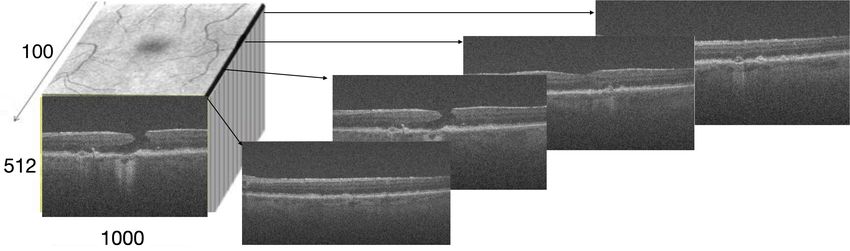
and output (label) [63]. This issue is particularly notable        mines the label. If we were provided with an image of a
in small-sample-size (weak supervision) scenarios or when          bird in an environment foreign to the images in the training
the sources of non-informative variation are overwhelming,         set, the model will be unable to make a reliable prediction,
thus likely to cause severe overfitting. These can lead to         thus causing robustness concerns. This generalization issue
catastrophic failures on deployment [19, 64].                      worsens with a smaller training sample size. On the other
    A growing recognition of the issues associated with the        hand, saliency maps from our PPI-enhanced model success-
lack of interpretable predictions is well documented in re-        fully focus on the bird anatomy, and thus will be robust to
cent years [1, 26, 43]. Such phenomenon has energized re-          environmental changes captured in the input images.
searchers to actively seek creative solutions. Among these,           PPI addresses causally-informed reasoning, robust learn-
two streams of work, namely saliency mapping [68, 54, 10]          ing, and model interpretation in a unified framework. A new
and causal representation learning (CRL) [28, 65, 2], stand        saliency mapping method, named Weight Back Propagation
out as some of the most promising directions. Specifically,        (WBP), is also proposed to generate more concentrated in-
saliency mapping encompasses techniques for post hoc vi-           tervention mask for PPI training. The key contributions of
sualizations on the input (image) space to facilitate the inter-   this paper include:
pretation of model predictions. This is done by projecting            • An end-to-end contrastive representation learning
the key features used in prediction back to the input space,            strategy PPI that employs proactive interventions to
resulting in the commonly known saliency maps. Impor-                   identify causally relevant features.
tantly, these maps do not directly contribute to model learn-
                                                                      • A fast and architecture-agnostic saliency mapping
ing. Alternatively, CRL solutions are built on the princi-
                                                                        module WBP that delivers better visualization and lo-
ples of establishing invariance from the data, and it entails
                                                                        calization performance.
teasing out sources of variation that are spuriously associ-
ated with the model output (labels). CRL models, while                • Experiments demonstrating significant performance
emphasizing the differences between causation and corre-                boosts from integrating PPI and WBP relative to com-
lation, are not subject to the rigor of causal inference ap-            peting solutions, especially on out-of-domain predic-
proaches, because their goal is not to obtain accurate causal           tions, data integration with heterogeneous sources and
effect estimates but rather to produce robust models with               model interpretation.
better generalization ability relative to their naively learned
counterparts [2].                                                  2. Background
    In this work, we present Proactive Pseudo-Intervention         Visual Explanations Saliency mapping collectively refers
(PPI), a solution that accounts for the needs of causal repre-     to a family of techniques to understand and interpret black-
sentation identification and visual verification. Our key in-      box image classification models, such as deep neural net-
sight is the derivation of causally-informed saliency maps,        works [1, 26, 43]. These methods project the model un-
which facilitate visual verification of model predictions and      derstanding of the targets, i.e., labels, and their predictions
enable learning that is robust to (non-causal) associations.       back to the input space, which allows for the visual inspec-
While true causation can only be established through ex-           tion of automated reasoning and for the communication of
perimental interventions, we leverage tools from contrastive       predictive visual cues to the user or human expert, aiming
representation learning to synthesize pseudo-interventions         to shed model insights or to build trust for deep-learning-
from observational data. Our procedure is motivated by the         based systems.
causal argument: perturbing the non-causal features will not           In this study, we focus on post hoc saliency map-
change the target label.                                           ping strategies, where saliency maps are constructed given
    To motivate, in Figure 1 we present an example to illus-       an arbitrary prediction model, as opposed to relying on
trate the benefits of producing causally-informed saliency         customized model architectures for interpretable predic-
maps. In this scenario, the task is to classify two bird           tions [19, 64], or to train a separate module to explicitly
species (A and B) in the wild. Due to the differences in their     produce model explanations [19, 21, 6, 18, 53]. Popu-
natural habitats, A-birds are mostly seen resting on rocks,        lar solutions under this category include: activation map-
while B-birds are more commonly found among bulrushes.             ping [69, 51], input sensitivity analysis [53], and rele-
A deep model, trained naively, will tend to associate the          vance propagation [4]. Activation mapping based methods
background characteristics with the labels, knowing these          fail at visualizing fine-grained evidence, which is particu-
strongly correlate with the bird species (labels) in the train-    larly important in explaining medical classification mod-
ing set. This is confirmed by the saliency maps derived from       els [14, 51, 60]. Input sensitivity analysis based meth-
the layer-wise relevance propagation (LRP) techniques [4]:         ods produce fine-grained saliency maps. However, these
the model also attends heavily on the background features,         maps are generally less concentrated [10, 18] and less inter-
while the difference in bird anatomy is what causally deter-       pretable. Relevance propagation based methods, like LRP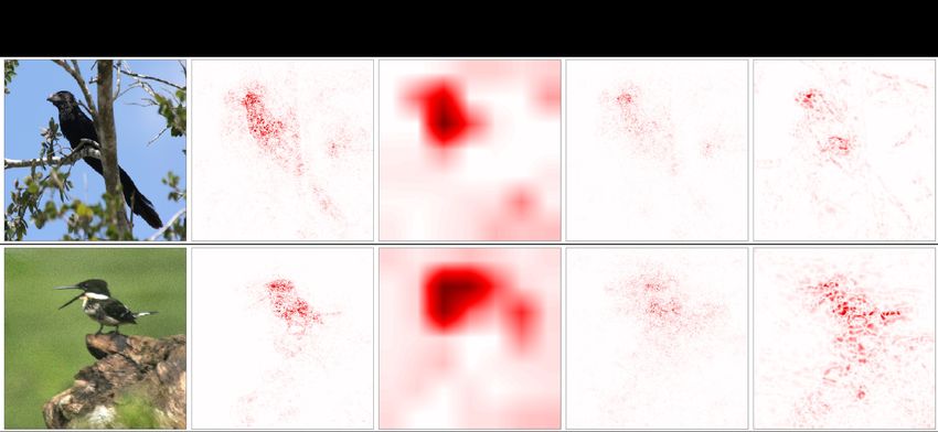
and its variants, use complex rules to prioritize positive or     the predictor and loss functions without introducing a new
large relevance, making the saliency maps visually appeal-        critic [59]. Notably, current CL methods are not immune
ing to human. However, our experiments demonstrate that           to spurious associations, a point we wish to improve in this
LRP and its variants highlight spuriously correlated features     work.
(boarderlines and backgrounds). By contrast, our WBP
backpropagates the weights through layers to compute the          Causality and Interventions. From a causality perspec-
contributions of each input pixel, which is truly faithful to     tive, humans learn via actively interacting with the environ-
the model, and WBP tends to highlight the target objects          ment. We intervene and observe changes in the outcome
themselves rather than the background. At the same time,          to infer causal dependencies. Machines instead learn from
the simplicity and efficiency makes WBP easily work with          static observations that are unable to inform the structural
other advanced learning strategies for both model diagnosis       dependencies for causal decisions. As such, perturbations
and improvements during training.                                 to the external factors, e.g., surroundings, lighting, view-
                                                                  ing angles, may drastically alter machine predictions, while
    Our work is in a similar spirit to [18, 10, 6, 60], where
                                                                  human recognition is less susceptible to such nuisance vari-
meaningful perturbations have been applied to the im-
                                                                  ations. Formally, such difference is
                                                                                                     Pbest explained with the
age during model training, to improve prediction and fa-
                                                                  do-notation [41]: P(Y |do(x)) = z P(Y |X = x, z)P(z),
cilitate interpretation. Poineering works have relied on
                                                                  where we identify x as the features, e.g., an object in the
user supplied “ground-truth” explainable masks to perturb
                                                                  image, and z as the confounders, e.g., background in the
[46, 35, 45], however such manual annotations are costly
                                                                  example above. Note that P(Y |do(x)) is fundamentally
and hence rarely available in practice. Alternatively, per-
                                                                  different from the conditional likelihood P(Y |X = x) =
turbations can be computed by solving an optimization for         P
each image. Such strategies are costly in practice and also          z P(Y |X = x, z)P(z|X = x), which machine uses for
                                                                  associative reasoning.
do not effectively block spurious features. Very recently,
exploratory effort has been made to leverage the tools from           Unfortunately, carrying out real interventional studies,
counterfactual reasoning [21] and causal analysis [40] to de-     i.e., randomized control trials, to intentionally block non-
rive visual explanations, but do not lend insights back to        causal associations, is oftentimes not a feasible option for
model training. Our work represents a fast, principled solu-      practical considerations, e.g., due to cost and ethics. This
tion that overcomes the above limitations. It automatically       work instead advocates the application of synthetic inter-
derives explainable masks faithful to the model and data,         ventions to uncover the underlying causal features from ob-
without explicit supervision from user-generated explana-         servational data. Specifically, we proactively edit x and its
tions.                                                            corresponding label y in a data-driven fashion to encourage
                                                                  the model to learn potential causal associations. Our pro-
Contrastive Learning. There has been growing interest             posal is in line with the growing appreciation for the signif-
in exploiting contrastive learning (CL) techniques for rep-       icance of establishing causality in machine learning models
resentations learning [39, 9, 24, 29, 59]. Originally devised     [49]. Via promoting invariance [2], such causally inspired
for density estimation [23], CL exploits the idea of learn-       solutions demonstrate superior robustness to superficial fea-
ing by comparison to capture the subtle features of data,         tures that do not generalize [62]. In particular, [57, 67]
i.e., positive examples, by contrasting them with negative        showed the importance and effectiveness of accounting for
examples drawn from a carefully crafted noise distribution.       interventional perspectives. Our work brings these causal
These techniques aim to avoid representation collapse, or to      views to construct a simple solution that explicitly opti-
promote representation consistency, for downstream tasks.         mizes visual interpretation and model robustness.
Recent developments, both empirical and theoretical, have
connected CL to information-theoretic foundations [59, 22],       3. Proactive Pseudo-Intervention
thus establishing them as a suite of de facto solutions for un-
supervised representation learning [9, 24].                           Below we describe the construction of Proactive
    The basic form of CL is essentially a binary classifica-      Pseudo-Intervention (PPI), a causally-informed contrastive
tion task specified to discriminate positive and negative ex-     learning scheme that seeks to simultaneously improve the
amples. In such a scenario, the binary classifier is known        accuracy, robustness, generalization and interpretability of
as the critic function. Maximizing the discriminative power       deep-learning-based computer vision models.
wrt the critic and the representation sharpens the feature en-        The PPI learning strategy, schematically summarized in
coder. Critical to the success of CL is the choice of ap-         Figure 2, consists of three main components: (i) a saliency
propriate noise distribution, where the challenging nega-         mapping module that highlights causally relevant features;
tives, i.e., those negatives that are more similar to positive    (ii) an intervention module that synthesizes contrastive
examples, are often considered more effective contrasts.          samples; and (iii) the prediction module, which is standard
In its more generalized form, CL can naturally repurpose          in recent vision models, e.g., VGG [55], ResNet [25], and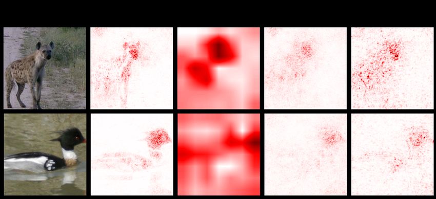
Figure 2: Illustration of the proposed PPI learning strategy. Input images are intervened by removing the saliency map based
masks, which alters the input label (e.g., negative control). For positive contrast, we use the original input as well as an input
masked with a random slaiency map. We use WBP for the generation of saliency maps.

Inception Net [58]. Motivated by the discussions from our          where σ and ω > 0 are the threshold and scaling param-
introduction, PPI establishes a feedback loop between the          eters, respectively. We set the scaling ω so that T (s) will
saliency map module and the prediction module, which is            result in a sharp transition from 0 to 1 near σ. Using (1) we
interfaced by the synthesized contrastive examples in the          define the contrastive loss as
intervention module. Under this configuration, the predic-                                      X
tion module is encouraged to modify its predictions only                           Lcon (θ) =      `(x∗i , ¬y; fθ ),          (3)
                                                                                                 i
when provided with causally-relevant synthetic interven-
tions. Note that components (i) and (ii) do not involve any        where fθ is the prediction module, `(x, y; fθ ) is the loss
additional parameters or neural network modules, which             function we wish to optimize, e.g. cross entropy, and ¬ is
makes our strategy readily applicable to the training of vir-      used to denote that the original class label has been flipped.
tually any computer vision task without major customiza-           In the binary case, ¬y = 1 − y, and in the multi-class case
tion. Details of these building blocks are given below.            it can be interpreted accordingly, e.g., using a one vs. oth-
3.1. Synthetic causal interventions for contrasts                  ers cross entropy loss. In practice, we set `(x, y; fθ ) =
                                                                   −`(x, y; fθ ). We will show in the experiments that this
   Key to our formulation is the design of a synthetic in-         simple and intuitive causal masking strategy works well in
tervention strategy that generates contrastive examples to         practice (see Tables 2 and 4, and Figure 4). Alternatively,
reinforce causal relevance during model training. Given a          we also consider a hard-masking approach in which a mini-
causal saliency map sm (x) for an input x wrt label y = m,         mal bounding box covering the thresholded saliency map is
where m = 1, . . . , M , and M is the number of classes, the       removed. See the Appendix for details.
synthetic intervention consists of removing (replacing with            Note that we are making the implicit assumption that the
zero) the causal information from x contained in sm (x),           saliency map is uniquely determined by the prediction mod-
and then using it as the contrastive learning signal.              ule fθ . While optimizing (3) explicitly attempts to improve
   For now, let us assume the causal salience map sm (x)           the fit of the prediction module fθ , it also implicitly informs
is known; the procedure to obtain the saliency map will be         the causal saliency mapping. This is sensible because if a
addressed in the next section. For notational clarity, we use      prediction is made using non-causal features, which implies
subscript i to denote entities associated with the i-th training   the associated saliency map sm (x) is also non-causal, then
sample, and omit the dependency on learnable parameters.           we should expect that after applying sm (x) to x using (1),
To remove causal information from xi and obtain a negative         we can still expect to make the correct prediction, i.e., the
contrast x∗i , we apply the following soft-masking                 true label, for both positive (the original) and negative (the
                                                                   intervened) samples.
                x∗i = xi − T (sm (xi ))     xi ,            (1)
                                                                   Saliency map regularization. Note that naively optimizing
where T (·) is a differentiable masking function and de-           (3) can lead to degenerate solutions for which any saliency
notes element-wise (Hadamard) multiplication. Specifi-             map that satisfies the causal sufficiency, i.e., encompassing
cally, we use the thresholded sigmoid for masking:                 all causal features, is a valid causal saliency map. For ex-
                                                                   ample, a trivial solution where the saliency map covers the
                                    1                              entire image may be considered causal. To protect against
        T (sm (xi )) =                             ,        (2)    such degeneracy, we propose to regularize the L1 -norm of
                         1 + exp(−ω(sm (xi ) − σ))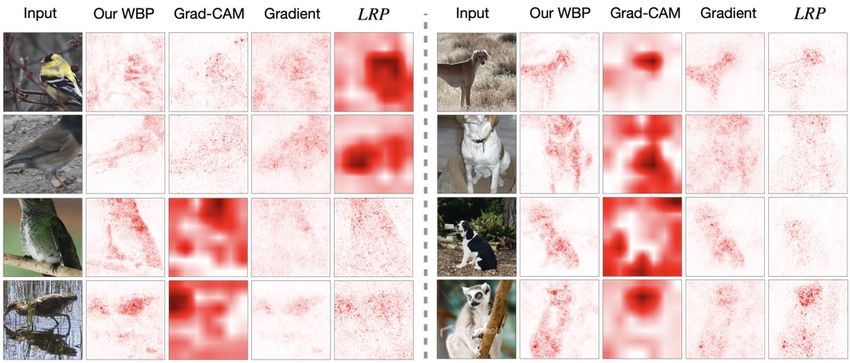
Table 1: WBP update rules for common transformations.                W̃ l , which we call the saliency matrix, satisfying,

    Transformation             G(·)                                                  xL = W̃ l xl ,   ∀l ∈ [0, . . . , L],         (6)
    Activation Layer           W̃ l = h ◦ W̃ l+1                      where xL is an M -dimensional vector corresponding to the
    FC Layer                   W̃ l = W̃ l+1 W l                      M distinct classes in y. Though presented in a matrix form
                                                     T0,1
    Convolutional Layer        W̃ l = W̃ l+1 ⊗ [W l ]f lip2,3
                                                                      in a slight abuse of notation, i.e., the instantiation of the op-
    BN Layer                   W̃ l = W̃σ γ
                                           l+1
                                                                      erator W̃ l effectively depends on the input x, thus all non-
    Pooling Layer              Relocate/Distribute W̃ l+1             linearities have been effectively absorbed into it. We posit
                                                                      that for an object associated with a given label y = m, its
                                                                      causal features are subsumed in the interactions between the
the saliency map to encourage succinct (sparse) representa-           m-th row of W̃ 0 and input x, i.e.,
tions, i.e., Lreg = ksm k1 , for m = 1, . . . , M .
                                                                                        [sm (x)]k = [W̃ 0 ]mk [x]k ,               (7)
Adversarial positive contrasts. Another concern with
solely optimizing (3) is that models can easily overfit to the        where [sm (x)]k denotes the k-th element of the saliency
intervention, i.e., instead of learning to capture causal rele-       map sm (x) and [W̃ 0 ]mk is a single element of W̃ 0 . A key
vance, the model learns to predict interventional operations.         observation for computation of W̃ l is that it can be done
For example, the model can learn to change its prediction             recursively. Specifically, let gl (xl ) be the transformation
when it detects that the input has been intervened, regard-           at the l-th layer, e.g., an affine transformation, convolution,
less of whether the image is missing causal features. So              activation, normalization, etc., then it holds that
motivated, we introduce adversarial positive contrasts:
                                                                                  W̃ l+1 xl+1 = W̃ l+1 gl (xl ) = W̃ l xl .        (8)
           x0i   = xi − T (sm (xj ))       xi ,    i 6= j,      (4)
                                                                      This allows for recursive computation of W̃ l via
where we intervene with a false saliency map, i.e., sm (xj )
is the saliency map from a different input xj , while still                         W̃ l = G(W̃ l+1 , gl ),   W̃ L = 1,            (9)
encouraging the model to make the correct prediction via
                               X                                      where G(·) is the update rule. We list the update rules for
                   Lad (θ) =       `(x0i , y; fθ ) ,            (5)   common transformations in deep networks in Table 1, with
                               i                                      corresponding derivations detailed below.
where x0i is the adversarial positive contrast. The complete
                                                                      Fully-connected (FC) layer. The FC transformation is the
loss for the proposed model, L = Lcls +Lcon +Lreg +Lad ,
                                                                      most basic operation in deep neural networks. Below we
consists of the contrastive loss in (3), the regularization loss,
                                                                      omit the bias term as it does not directly interact with the
Lreg , and the adversarial loss in (5).
                                                                      input. Assuming gl (xl ) = W l xl , it is readily seen that
3.2. Saliency Weight Backpropagation
                                                                           W̃ l+1 xl+1 = W̃ l+1 gl (xl ) = (W̃ l+1 W l )xl ,      (10)
    In order to generate saliency maps that inform decision-
driving features in the (raw) pixel space, we describe                so W̃ l = W̃ l+1 W l . Graphical illustration with standard
Weight Back Propagation (WBP), a novel computationally                affine mapping and ReLU activation can be found in the
efficient scheme for saliency mapping applicable to arbi-             appendix.
trary neural architectures. WBP evaluates individual contri-
                                                                      Nonlinear activation layer. Considering that an activa-
butions from each pixel to the final class-specific prediction,
                                                                      tion layer simply rescales the saliency weight matrices, i.e.,
and we empirically find the results to be more causally-
                                                                      xl+1 = gl (xl ) = hl ◦ xl , where ◦ is the composition opera-
relevant relative to competing solutions based on human
                                                                      tor, we obtain W̃ l = h ◦ W̃ l+1 . Using the ReLU activation
judgement.
                                                                      as a concrete example, we have h(xl ) = 1{xl ≥ 0}.
    To simplify our presentation, we first consider a vector
input and a linear mapping. Let xl be the internal repre-             Convolutional layer. The convolution is a generalized form
sentation of the data at the l-th layer, with l = 0 being             of linear mapping. In practice, convolutions can be ex-
the input layer, i.e., x0 = x, and l = L being the penul-             pressed as tensor products of the form W̃ l = W̃ l+1 ⊗
                                                                            T0,1
timate logit layer prior to the softmax transformation, i.e.,         [W l ]f lip2,3
                                                                                     , where W l ∈ RD2 ×D1 ×(2S+1)×(2S+1) is the
P(y|x) = softmax(xL ). To assign the relative importance              convolution kernel, T0,1 is the transpose in dimensions 0
to each hidden unit in the l-th layer, we notationally col-           and 1 and f lip2,3 is an exchange in dimensions 2 and 3.
lapse all transformations after l into an operator denoted by         See the Appendix for details.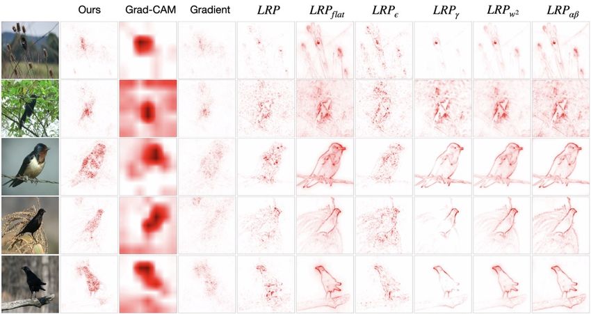
Figure 3: Visualization of the inferred saliency maps. Left: CUB dataset. Right: ImageNet dataset.

Pooling and normalization layer. Summarization and               Table 2: Performance improvements achieved by training
standardization are two other essential operations for the       with PPI on CUB, CIFAR-10, and GA dataset. We re-
success of deep neural networks, achieved by pooling and         port means and standard deviations (SDs) from 5-fold cross-
batch normalization (BN) techniques, respectively. They          validation for GA prediction.
too can be considered as special instantiations of linear op-
erations. Here we summarize the two most popular opera-            Models             CUB     Cifar-10    GA
tions in Table 1.                                                                     (Acc)   (Acc)       (AUC)
                                                                   Classification     0.662   0.881       0.877 ± 0.040
4. Experiments                                                     +PPIGradient       0.673   0.885       0.890 ± 0.035
    To validate the utility of our approach, we consider both      +PPILRP            0.680   0.891       0.895 ± 0.037
natural and medical image datasets, and compare it to ex-          +PPIGradCAM        0.683   0.895       0.908 ± 0.036
isting state-of-the-art solutions. All the experiments are im-     +PPIW BP           0.696   0.901       0.925 ± 0.023
plemented in PyTorch. The source code will be available at
https://github.com/author_name/PPI. Due to                       for details about the masking parameters σ and ω.
space limitation, details of the experimental setup and addi-
tional analyses are deferred to the Appendix.                    4.1. Natural Image Datasets
Datasets. We present our findings on five represen-              Classification Gains In this experiment, we investigate
tative datasets: (i) CIFAR-10 [31]; (ii) ImageNet                how the different pairings of PPI and saliency mapping
(ILSVRC2012) [47]; (iii) CUB [61], a natural image               schemes (i.e., GradCAM, LRP, WBP) affect performance.
dataset with over 12k photos for classification of 200 bird      In Table 2, the first row represents VGG11 model trained
species in the wild, heavily confounded by the background        with only classification loss, and the following rows repre-
characteristics; (iv) GA [34], a new medical image dataset       sent VGG11 trained with PPI with different saliency map-
for the prediction of geographic atrophy (GA) using 3D op-       ping schemes. We see consistent performance gains in ac-
tical coherence tomography (OCT) image volumes, char-            curacy via incorporating PPI training on both CUB and
acterized by small sample size (275 subjects) and highly         CIFAR-10 datasets. The gains are mostly significant when
heterogeneous (collected from 4 different facilities); and       using our WBP for saliency mapping (improving the accu-
(v) LIDC-IDRI [33], a public medical dataset of 1, 085           racy from 0.662 to 0.696 on CUB, and from 0.881 to 0.901
lung lesion CT images annotated by 4 radiologists. Detailed      on CIFAR-10.
specifications are described in the Appendix.                    Model Interpretability In this task, we want to qualita-
                                                                 tively and quantitatively compare the causal relevance of
Baselines. The following set of popular saliency mapping
                                                                 saliency maps generated by our proposed model and its
schemes are considered as comparators for the proposed ap-
                                                                 competitors. In Figure 3, we show the saliency maps
proach: (i) Gradient: standard gradient-based salience map-
                                                                 produced by different approaches for a VGG11 model
ping; (ii) GradCAM [51]: gradient-weighted class activa-
                                                                 trained on CUB. Visually, gradient-based solutions (Grad
tion mapping; (iii) LRP [4]: layer-wise relevance propaga-
                                                                 and GradCAM) tend to yield overly dispersed maps, in-
tion and its variants.
                                                                 dicating a lack of specificity. LRP gives more appealing
Hyperparameters. The final loss of the proposed model is         saliency maps. However, these maps also heavily attend
a weighted summation of four losses: L = Lcls +w1 Lcon +         to the spurious background cues that presumably help with
w2 Lreg +w3 Lad . The weights are simply balanced to match       predictions. When trained with PPI, the saliency maps at-
the magnitude of Lcls , i.e., w3 = 1, w2 = 0.1 and w1 = 1        tend to birds body, and with WBP, the saliency maps focus
(CUB), = 1 (GA), and = 10 (LIDC). See Appendix Sec B             on the causal related pixels.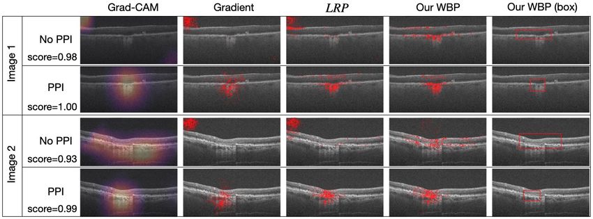
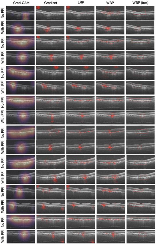
Figure 4: Saliency maps on GA dataset based on models trained with PPI and without PPI. Maps of models trained with PPI
are more clinically relevant by focusing on retinal layers likely to contain abnormalities or lesions, and more concentrated.

    To quantitatively evaluate the causal relevance of com-
peting saliency maps, we adopt the evaluation scheme pro-
posed in [26], consisting of masking out the contribut-
ing saliency pixels and then calculating the reduction in
prediction score. A larger reduction is considered better
for accurately capturing the pixels that ‘cause’ the pre-
diction. Results are summarized in Figure 5a, where we
progressively remove the top-k saliency points, with k =
100, 500, 1000, 5000, 10000 (10000 ≈ 6.6% of all pixels),                    (a) CUB                    (b) ImageNet
from the CUB test input images. Our PPI consistently out-         Figure 5: Quantitative evaluations of causal relevance of
performs its counterparts, with its lead being most substan-      competing saliency maps (higher is better).
tial in the low-k regime. Notably, for large k, PPI removes
nearly all predictive signal. This implies PPI specifically
targets the causal features. Quantitative evaluation with ad-     saliency mapping schemes (i.e., Grad, GradCAM, LRP,
ditional metrics are provided in the Appendix.                    WBP) work with PPI. For WBP, we also tested the bound-
    To test the performance of WBP itself (without being          ing box variant, denoted as WBP (box) (see the Appendix
trained with PPI), we compare WBP with different ap-              for details). In Table 2, we see consistent performance gains
proaches for a VGG11 model trained on ImageNet from Py-           in AUC score via incorporating PPI training (from 0.877 to
Torch model zoo. Figure 3(left) shows that saliency maps          0.925, can be improve to 0.937 by PPI with WBP(box)),
generated by WBP more concentrate on objects themselves.          accompanied by the reductions in model variation evalu-
Also, thanks to the fine resolution of WBP, the model pays        ated by the standard deviations of AUC from the five-fold
more attention to the patterns on the fur to identify the leop-   cross-validation. The gains are most significant when us-
ard (row 1). This is more visually consistent with human          ing our WBP for saliency mapping. We further compare the
judgement. Figure 5b demonstrates WBP identifies more             saliency maps generated by these different combinations.
causal pixels on ImageNet validation images.                      We see that without the additional supervision from PPI,
                                                                  competing solutions like Grad, GradCAM and LRP some-
4.2. OCT-GA: Geographic Atrophy Classification
                                                                  times yield non-sensible saliency maps (attending to im-
    Next we show how the proposed PPI handles the chal-           age corners). Overall, PPI encourages more concentrated
lenges of small training data and heterogeneity in medical        and less noisy saliency maps. Also, different PPI-based
image datasets. In this experiment (with our new dataset,         saliency maps agree with each other to a larger extent. Our
that we will make public), each OCT volume image con-             findings are also verified by experts (co-authors, who are
sists of 100 scans of a 512 × 1000 sized image [5]. We            ophthalmologists specializing in GA) confirming that the
use a multi-view CNN model [56] to process such 3D                PPI-based saliency maps are clinically relevant by focusing
OCT inputs, and use it as our baseline solution (see the          on retinal layers likely to contain abnormalities or lesions.
Appendix for details). We investigate how the different           These results underscore the practical value of the proposed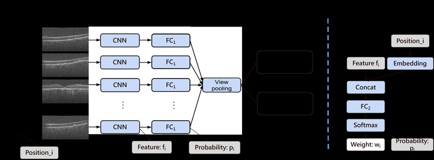
Table 3: AUC results for GA prediction with or without
PPI. Models are trained on one site and cross-validated on
the other sites. Darker color indicates better performance.

With PPI    A        B        C         D        Mean     STD
A            1.000   0.906    0.877     0.865    0.912    0.061
B           0.851    0.975    0.863     0.910    0.900    0.056
C           0.954    0.875    0.904     0.931    0.916    0.034
D           0.824    0.846    0.853     0.904    0.857    0.034
No PPI      A        B        C         D        Mean     STD
A           1.000    0.854    0.832     0.827    0.878    0.082
B           0.810    0.874    0.850     0.906    0.860    0.040
                                                                  Figure 6: Saliency maps on LIDC-IDR. Saliency maps of
C           0.860    0.779    0.873     0.862    0.843    0.043
                                                                  PPI+WBP are mostly consistent with the ground truths.
D           0.748    0.792    0.836     0.961    0.834    0.092
                                                                  setup from [50] to predict
proactive interventions.                                          lesions. We use Incep-
Cross-domain generalization. Common to medical im-                tion v3 [58] as our base model for both standard classifica-
age applications is that training samples are usually inte-       tion and PPI-enhanced training with various saliency map-
grated from a number of healthcare facilities (i.e., domains),    ping schemes. See the Appendix for details.
and that predictions are sometimes to be made on sub-
jects at other facilities. Despite big efforts to standardize     Lesion classification. We first compare PPI to other spe-
the image collection protocols, with different imaging sys-       cialized SOTA network architectures. Table 4 summa-
tems operated by technicians with varying skills, apparent        rizes AUC scores of Tensor Net-X [15], DenseNet [27],
domain shifts are likely to compromise the cross-domain           LoTeNet [50], Inception v3 [58], as well as our Incep-
performance of these models. We show this phenomenon              tion v3 trained with and without PPIW BP . The proposed
on the GA dataset in Table 3, where source samples are            PPIW BP (box) leads the performance chart by a considerable
collected from four different hospitals in different health       margin, improving Inception v3 from 0.92 to 0.94.
systems (A, B, C and D, see the Appendix for details).            Weakly-supervised image segmentation. In Figure 6,
Each cell contains the AUC of the model trained on site           we compare saliency maps generated by GradCAM, WBP,
X (row) and tested on site Y (column), with same-site pre-        WBP (box) to the ground truth lesion masks from expert
dictions made on hold-out samples. A significant perfor-          annotations. Note that we have only supplied patch-label
mance drop is observed for cross-domain predictions (off-         labels during training, not the pixel-level expert segmenta-
diagonals) compared to in-domain predictions (diagonals).         tion masks, which constitute a challenging task of weakly-
With the application of PPI, the performance gaps between         supervised image segmentation. In line with the observa-
in-domain and cross-domain predictions are considerably           tions from the GA experiment, our PPI-training enhanced
reduced. The overall accuracy gains of PPI further justify        WBP saliency maps are mostly consistent with the expert
the utility of causally-inspired modeling. Notably, site D        segmentations. Together with Table 4, Figure 6 confirms
manifests strong spurious correlation that help in-domain         that the proposed PPI+WBP improves both the classifica-
prediction but degrades out-of-site generalization, which is      tion performance and model interpretability.
partly resolved by the proposed PPI.
4.3. LIDC-IDRI: Lung Lesions Classification                       5. Conclusions
   To further examine the         Table 4: LIDC-IDRI clas-            We have presented Proactive Pseudo-Intervention (PPI),
practical advantages of the       sification AUC results.         a novel interpretable computer vision framework that organ-
proposed PPI in real-world                                        ically integrates saliency mapping, causal reasoning, syn-
applications, we bench-               Models              AUC     thetic intervention and contrastive learning. PPI couples
mark its utility on LIDC-             Tensor Net-X [15]   0.823   saliency mapping with contrastive training by creating ar-
IDRI; a public lung CT                DenseNet [27]       0.829   tificially intervened negative samples absent of causal fea-
scan dataset [3].       We            LoTeNet [50]        0.874   tures. To communicate model insights and facilitate causal-
followed the preprocess-              Inception v3 [58]   0.921   informed reasoning, we derived an architecture-agnostic
                                      +PPIGradCAM         0.933
ing steps outlined in [30]                                        saliency mapping scheme called Weight Back Propagation
                                      +PPIGradient        0.930
to prepare the data, and              +PPILRP             0.931   (WBP), which faithfully captures the causally-relevant pix-
adopted the experimental              +PPIW BP            0.935   els/features for model prediction. Visual inspection of the
                                      +PPIW BP (box)      0.941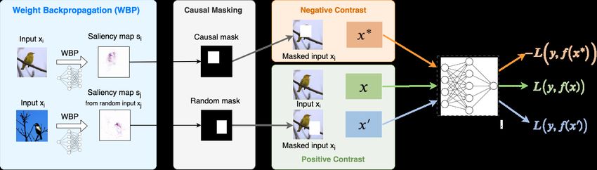
saliency maps show that WBP, is more robust to spurious                       Processing Systems, pages 6967–6976, 2017. 2, 3, 12, 13,
features compared to competing approaches. Empirical re-                      14
sults on natural and medical datasets verify the combination           [11]   Jia Deng, Wei Dong, Richard Socher, Li-Jia Li, Kai Li,
of PPI and WBP consistently delivers performance boosts                       and Li Fei-Fei. Imagenet: A large-scale hierarchical image
across a wide range of tasks relative to competing solutions,                 database. In 2009 IEEE conference on computer vision and
and the gains are most significant where the application is                   pattern recognition, pages 248–255. Ieee, 2009. 1
complicated by small sample size, data heterogeneity, or               [12]   Li Deng. The mnist database of handwritten digit images for
                                                                              machine learning research [best of the web]. IEEE Signal
confounded with spurious correlations.
                                                                              Processing Magazine, 29(6):141–142, 2012. 1
                                                                       [13]   Amit Dhurandhar, Pin-Yu Chen, Ronny Luss, Chun-Chen
References                                                                    Tu, Paishun Ting, Karthikeyan Shanmugam, and Payel Das.
 [1] Julius Adebayo, Justin Gilmer, Michael Muelly, Ian Good-                 Explanations based on the missing: Towards contrastive ex-
     fellow, Moritz Hardt, and Been Kim. Sanity checks for                    planations with pertinent negatives. In Advances in Neural
     saliency maps. In Advances in Neural Information Process-                Information Processing Systems, pages 592–603, 2018. 14
     ing Systems, pages 9505–9515, 2018. 2                             [14]   Mengnan Du, Ninghao Liu, Qingquan Song, and Xia Hu. To-
 [2] Martin Arjovsky, Léon Bottou, Ishaan Gulrajani, and David               wards explanation of dnn-based prediction with guided fea-
     Lopez-Paz. Invariant risk minimization. arXiv preprint                   ture inversion. In Proceedings of the 24th ACM SIGKDD
     arXiv:1907.02893, 2019. 2, 3                                             International Conference on Knowledge Discovery & Data
 [3] Samuel G Armato III, Geoffrey McLennan, Luc Bidaut,                      Mining, pages 1358–1367, 2018. 2, 12, 13
     Michael F McNitt-Gray, Charles R Meyer, Anthony P                 [15]   Stavros Efthymiou, Jack Hidary, and Stefan Leichenauer.
     Reeves, Binsheng Zhao, Denise R Aberle, Claudia I Hen-                   Tensornetwork for machine learning.           arXiv preprint
     schke, Eric A Hoffman, et al. The lung image database con-               arXiv:1906.06329, 2019. 8
     sortium (lidc) and image database resource initiative (idri):     [16]   Dumitru Erhan, Yoshua Bengio, Aaron Courville, and Pascal
     a completed reference database of lung nodules on ct scans.              Vincent. Visualizing higher-layer features of a deep network.
     Medical physics, 38(2):915–931, 2011. 8, 17                              University of Montreal, 1341(3):1, 2009. 13
 [4] Sebastian Bach, Alexander Binder, Grégoire Montavon,             [17]   Ruth Fong, Mandela Patrick, and Andrea Vedaldi. Un-
     Frederick Klauschen, Klaus-Robert Müller, and Wojciech                  derstanding deep networks via extremal perturbations and
     Samek. On pixel-wise explanations for non-linear classi-                 smooth masks. In Proceedings of the IEEE International
     fier decisions by layer-wise relevance propagation. PloS one,            Conference on Computer Vision, pages 2950–2958, 2019. 12
     10(7):e0130140, 2015. 2, 6, 13                                    [18]   Ruth C Fong and Andrea Vedaldi. Interpretable explanations
 [5] David S Boyer, Ursula Schmidt-Erfurth, Menno van Look-                   of black boxes by meaningful perturbation. In Proceedings
     eren Campagne, Erin C Henry, and Christopher Brittain. The               of the IEEE International Conference on Computer Vision,
     pathophysiology of geographic atrophy secondary to age-                  pages 3429–3437, 2017. 2, 3, 12, 13, 14
     related macular degeneration and the complement pathway           [19]   Hiroshi Fukui, Tsubasa Hirakawa, Takayoshi Yamashita, and
     as a therapeutic target. Retina (Philadelphia, Pa.), 37(5):819,          Hironobu Fujiyoshi. Attention branch network: Learning
     2017. 7, 15                                                              of attention mechanism for visual explanation. In Proceed-
 [6] Chun-Hao Chang, Elliot Creager, Anna Goldenberg, and                     ings of the IEEE Conference on Computer Vision and Pattern
     David Duvenaud. Explaining image classifiers by counter-                 Recognition, pages 10705–10714, 2019. 2, 13, 14
     factual generation. In International Conference on Learning       [20]   Ross Girshick, Jeff Donahue, Trevor Darrell, and Jitendra
     Representations, 2018. 2, 3, 13, 14                                      Malik. Rich feature hierarchies for accurate object detection
 [7] Aditya Chattopadhay, Anirban Sarkar, Prantik Howlader,                   and semantic segmentation. In Proceedings of the IEEE con-
     and Vineeth N Balasubramanian. Grad-cam++: General-                      ference on computer vision and pattern recognition, pages
     ized gradient-based visual explanations for deep convolu-                580–587, 2014. 1
     tional networks. In 2018 IEEE Winter Conference on Appli-         [21]   Yash Goyal, Ziyan Wu, Jan Ernst, Dhruv Batra, Devi Parikh,
     cations of Computer Vision (WACV), pages 839–847. IEEE,                  and Stefan Lee. Counterfactual visual explanations. In
     2018. 13                                                                 ICML, 2019. 2, 3, 13, 14
 [8] Chenyi Chen, Ari Seff, Alain Kornhauser, and Jianxiong            [22]   Jean-Bastien Grill, Florian Strub, Florent Altché, Corentin
     Xiao. Deepdriving: Learning affordance for direct percep-                Tallec, Pierre Richemond, Elena Buchatskaya, Carl Doersch,
     tion in autonomous driving. In Proceedings of the IEEE                   Bernardo Avila Pires, Zhaohan Guo, Mohammad Ghesh-
     International Conference on Computer Vision, pages 2722–                 laghi Azar, et al. Bootstrap your own latent-a new approach
     2730, 2015. 1                                                            to self-supervised learning. Advances in Neural Information
 [9] Ting Chen, Simon Kornblith, Mohammad Norouzi, and Ge-                    Processing Systems, 33, 2020. 3
     offrey Hinton. A simple framework for contrastive learning        [23]   Michael Gutmann and Aapo Hyvärinen. Noise-contrastive
     of visual representations. arXiv preprint arXiv:2002.05709,              estimation: A new estimation principle for unnormalized
     2020. 3                                                                  statistical models. In Proceedings of the Thirteenth Inter-
[10] Piotr Dabkowski and Yarin Gal. Real time image saliency                  national Conference on Artificial Intelligence and Statistics,
     for black box classifiers. In Advances in Neural Information             pages 297–304, 2010. 3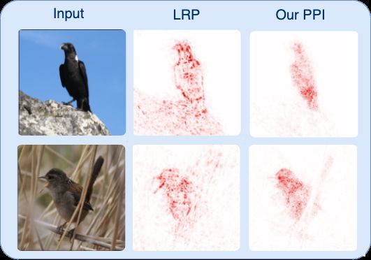
[24] Kaiming He, Haoqi Fan, Yuxin Wu, Saining Xie, and Ross                  AI: Interpreting, Explaining and Visualizing Deep Learning,
     Girshick. Momentum contrast for unsupervised visual rep-                pages 253–265. Springer, 2019. 13
     resentation learning. In Proceedings of the IEEE/CVF Con-        [38]   Grégoire Montavon, Alexander Binder, Sebastian La-
     ference on Computer Vision and Pattern Recognition, pages               puschkin, Wojciech Samek, and Klaus-Robert Müller.
     9729–9738, 2020. 3                                                      Layer-wise relevance propagation: an overview. In Explain-
[25] Kaiming He, Xiangyu Zhang, Shaoqing Ren, and Jian Sun.                  able AI: interpreting, explaining and visualizing deep learn-
     Deep residual learning for image recognition. In Proceed-               ing, pages 193–209. Springer, 2019. 13
     ings of the IEEE conference on computer vision and pattern       [39]   Aaron van den Oord, Yazhe Li, and Oriol Vinyals. Repre-
     recognition, pages 770–778, 2016. 3                                     sentation learning with contrastive predictive coding. arXiv
[26] Sara Hooker, Dumitru Erhan, Pieter-Jan Kindermans, and                  preprint arXiv:1807.03748, 2018. 3
     Been Kim. A benchmark for interpretability methods in deep       [40]   Matthew O’Shaughnessy, Gregory Canal, Marissa Connor,
     neural networks. In Advances in Neural Information Pro-                 Christopher Rozell, and Mark Davenport. Generative causal
     cessing Systems, pages 9737–9748, 2019. 1, 2, 7                         explanations of black-box classifiers. Advances in Neural
[27] Gao Huang, Zhuang Liu, Laurens Van Der Maaten, and Kil-                 Information Processing Systems, 33, 2020. 3, 13
     ian Q Weinberger. Densely connected convolutional net-           [41]   Judea Pearl. Causality. Cambridge university press, 2009. 3
     works. In Proceedings of the IEEE conference on computer         [42]   Vitali Petsiuk, Abir Das, and Kate Saenko. Rise: Random-
     vision and pattern recognition, pages 4700–4708, 2017. 8                ized input sampling for explanation of black-box models.
[28] Fredrik Johansson, Uri Shalit, and David Sontag. Learning               arXiv preprint arXiv:1806.07421, 2018. 12
     representations for counterfactual inference. In International
                                                                      [43]   Sylvestre-Alvise Rebuffi, Ruth Fong, Xu Ji, and Andrea
     conference on machine learning, pages 3020–3029, 2016. 2
                                                                             Vedaldi. There and back again: Revisiting backpropagation
[29] Prannay Khosla, Piotr Teterwak, Chen Wang, Aaron Sarna,
                                                                             saliency methods. In Proceedings of the IEEE/CVF Con-
     Yonglong Tian, Phillip Isola, Aaron Maschinot, Ce Liu, and
                                                                             ference on Computer Vision and Pattern Recognition, pages
     Dilip Krishnan. Supervised contrastive learning. arXiv
                                                                             8839–8848, 2020. 1, 2
     preprint arXiv:2004.11362, 2020. 3
                                                                      [44]   Marco Tulio Ribeiro, Sameer Singh, and Carlos Guestrin.
[30] Simon Kohl, Bernardino Romera-Paredes, Clemens Meyer,
                                                                             ” why should i trust you?” explaining the predictions of any
     Jeffrey De Fauw, Joseph R Ledsam, Klaus Maier-Hein,
                                                                             classifier. In Proceedings of the 22nd ACM SIGKDD interna-
     SM Ali Eslami, Danilo Jimenez Rezende, and Olaf Ron-
                                                                             tional conference on knowledge discovery and data mining,
     neberger. A probabilistic u-net for segmentation of ambigu-
                                                                             pages 1135–1144, 2016. 12
     ous images. In Advances in Neural Information Processing
     Systems, pages 6965–6975, 2018. 8, 17                            [45]   Laura Rieger, Chandan Singh, William Murdoch, and Bin
                                                                             Yu. Interpretations are useful: penalizing explanations to
[31] Alex Krizhevsky, Geoffrey Hinton, et al. Learning multiple
                                                                             align neural networks with prior knowledge. In International
     layers of features from tiny images. 2009. 1, 6
                                                                             Conference on Machine Learning, pages 8116–8126. PMLR,
[32] Alex Krizhevsky, Ilya Sutskever, and Geoffrey E Hinton.
                                                                             2020. 3
     Imagenet classification with deep convolutional neural net-
     works. Communications of the ACM, 60(6):84–90, 2017. 1           [46]   Andrew Slavin Ross, Michael C Hughes, and Finale Doshi-
[33] Curtis P Langlotz, Bibb Allen, Bradley J Erickson, Jayashree            Velez. Right for the right reasons: training differentiable
     Kalpathy-Cramer, Keith Bigelow, Tessa S Cook, Adam E                    models by constraining their explanations. In Proceedings
     Flanders, Matthew P Lungren, David S Mendelson, Jef-                    of the 26th International Joint Conference on Artificial Intel-
     frey D Rudie, et al. A roadmap for foundational research                ligence, pages 2662–2670, 2017. 3
     on artificial intelligence in medical imaging: from the 2018     [47]   Olga Russakovsky, Jia Deng, Hao Su, Jonathan Krause, San-
     nih/rsna/acr/the academy workshop. Radiology, 291(3):781–               jeev Satheesh, Sean Ma, Zhiheng Huang, Andrej Karpathy,
     791, 2019. 6                                                            Aditya Khosla, Michael Bernstein, Alexander C. Berg, and
[34] Jessica N Leuschen, Stefanie G Schuman, Katrina P Winter,               Li Fei-Fei. ImageNet Large Scale Visual Recognition Chal-
     Michelle N McCall, Wai T Wong, Emily Y Chew, Thomas                     lenge. International Journal of Computer Vision (IJCV),
     Hwang, Sunil Srivastava, Neeru Sarin, Traci Clemons, et al.             115(3):211–252, 2015. 6
     Spectral-domain optical coherence tomography characteris-        [48]   Paul Sajda. Machine learning for detection and diagnosis of
     tics of intermediate age-related macular degeneration. Oph-             disease. Annu. Rev. Biomed. Eng., 8:537–565, 2006. 1
     thalmology, 120(1):140–150, 2013. 6, 15                          [49]   Bernhard Schölkopf. Causality for machine learning. arXiv
[35] Kunpeng Li, Ziyan Wu, Kuan-Chuan Peng, Jan Ernst, and                   preprint arXiv:1911.10500, 2019. 3
     Yun Fu. Tell me where to look: Guided attention inference        [50]   Raghavendra Selvan and Erik B Dam. Tensor networks for
     network. In Proceedings of the IEEE Conference on Com-                  medical image classification. In Medical Imaging with Deep
     puter Vision and Pattern Recognition, pages 9215–9223,                  Learning, 2020. 8, 17
     2018. 3, 13                                                      [51]   Ramprasaath R Selvaraju, Michael Cogswell, Abhishek Das,
[36] Aravindh Mahendran and Andrea Vedaldi. Salient decon-                   Ramakrishna Vedantam, Devi Parikh, and Dhruv Batra.
     volutional networks. In European Conference on Computer                 Grad-cam: Visual explanations from deep networks via
     Vision, pages 120–135. Springer, 2016. 13                               gradient-based localization. In Proceedings of the IEEE In-
[37] Grégoire Montavon. Gradient-based vs. propagation-based                ternational Conference on Computer Vision, pages 618–626,
     explanations: an axiomatic comparison. In Explainable                   2017. 2, 6, 13
[52] Dasom Seo, Kanghan Oh, and Il-Seok Oh. Regional multi- [65] Tan Wang, Jianqiang Huang, Hanwang Zhang, and Qianru
scale approach for visually pleasing explanations of deep Sun. Visual commonsense representation learning via causal
neural networks. IEEE Access, 8:8572–8582, 2019. 12 inference. In Proceedings of the IEEE/CVF Conference on
[53] Avanti Shrikumar, Peyton Greenside, and Anshul Kundaje. Computer Vision and Pattern Recognition Workshops, pages
Learning important features through propagating activation 378–379, 2020. 2
differences. In International Conference on Machine Learn- [66] Matthew D Zeiler and Rob Fergus. Visualizing and under-
ing, pages 3145–3153, 2017. 2, 13 standing convolutional networks. In European conference on
[54] Karen Simonyan, Andrea Vedaldi, and Andrew Zisserman. computer vision, pages 818–833. Springer, 2014. 12
Deep inside convolutional networks: Visualising image [67] Cheng Zhang, Kun Zhang, and Yingzhen Li. A causal
classification models and saliency maps. arXiv preprint view on robustness of neural networks. arXiv preprint
arXiv:1312.6034, 2013. 2 arXiv:2005.01095, 2020. 3
[55] Karen Simonyan and Andrew Zisserman. Very deep convo- [68] Yitian Zhao, Yalin Zheng, Yifan Zhao, Yonghuai Liu, Zhili
lutional networks for large-scale image recognition. arXiv Chen, Peng Liu, and Jiang Liu. Uniqueness-driven saliency
preprint arXiv:1409.1556, 2014. 3 analysis for automated lesion detection with applications to
[56] Hang Su, Subhransu Maji, Evangelos Kalogerakis, and Erik retinal diseases. In International Conference on Medical Im-
Learned-Miller. Multi-view convolutional neural networks age Computing and Computer-Assisted Intervention, pages
for 3d shape recognition. In Proceedings of the IEEE in- 109–118. Springer, 2018. 2
ternational conference on computer vision, pages 945–953, [69] Bolei Zhou, Aditya Khosla, Agata Lapedriza, Aude Oliva,
2015. 7, 16 and Antonio Torralba. Learning deep features for discrimina-
[57] Raphael Suter, Djordje Miladinovic, Bernhard Schölkopf, tive localization. In Proceedings of the IEEE conference on
and Stefan Bauer. Robustly disentangled causal mecha- computer vision and pattern recognition, pages 2921–2929,
nisms: Validating deep representations for interventional ro- 2016. 2
bustness. In International Conference on Machine Learning,
pages 6056–6065. PMLR, 2019. 3
[58] Christian Szegedy, Vincent Vanhoucke, Sergey Ioffe, Jon
Shlens, and Zbigniew Wojna. Rethinking the inception archi-
tecture for computer vision. In Proceedings of the IEEE con-
ference on computer vision and pattern recognition, pages
2818–2826, 2016. 4, 8, 17
[59] Yonglong Tian, Dilip Krishnan, and Phillip Isola. Con-
trastive multiview coding. arXiv preprint arXiv:1906.05849,
2019. 3
[60] Jorg Wagner, Jan Mathias Kohler, Tobias Gindele, Leon Het-
zel, Jakob Thaddaus Wiedemer, and Sven Behnke. Inter-
pretable and fine-grained visual explanations for convolu-
tional neural networks. In Proceedings of the IEEE Con-
ference on Computer Vision and Pattern Recognition, pages
9097–9107, 2019. 2, 3, 12, 13
[61] C. Wah, S. Branson, P. Welinder, P. Perona, and S. Belongie.
The Caltech-UCSD Birds-200-2011 Dataset. Technical Re-
port CNS-TR-2011-001, California Institute of Technology,
2011. 6
[62] Haohan Wang, Zexue He, Zachary C Lipton, and Eric P
Xing. Learning robust representations by projecting super-
ficial statistics out. InInternational Conference on Learning
Representations, 2019. 3
[63] Haofan Wang, Zifan Wang, Mengnan Du, Fan Yang, Zijian
Zhang, Sirui Ding, Piotr Mardziel, and Xia Hu. Score-cam:
Score-weighted visual explanations for convolutional neural
networks. In Proceedings of the IEEE/CVF Conference on
Computer Vision and Pattern Recognition Workshops, pages
24–25, 2020. 2, 15
[64] Lezi Wang, Ziyan Wu, Srikrishna Karanam, Kuan-Chuan
Peng, Rajat Vikram Singh, Bo Liu, and Dimitris N Metaxas.
Sharpen focus: Learning with attention separability and con-
sistency. In Proceedings of the IEEE International Confer-
ence on Computer Vision, pages 512–521, 2019. 2, 14A. Weight Backpropagation (WBP) soft masking, we set ω to 100 and σ to 0.25. We have also
experimented with image-adaptive thresholds instead of a
A.1. Graphical illustration of WBP fixed σ for all inputs, i.e., set the threshold as mean value
See Figure 7 for a graphical illustration with standard plus k times of the standard deviation of WBP weights of
affine mapping and ReLU activation. the whole image. We repeat the experiments a few times
and the results are consistent. The experiment comparison
A.2. Derivation of Convolutional Weight Backprop- of these masking methods mention above is conducted on
agation LIDC dataset.
Let’s denote the input variable as I ∈ RH×W , the Table 5: Different causal masking methods on LIDC
convolutional filter weight as W ∈ R(2S+1)×(2S+1) , the
output variable as O ∈ RH×W , and the weight back- Models AUC
propagate to O as Ŵ ∈ RH×W . We omit the bias here
because it does not directly interact with the input vari- WBP-soft (fixed σ) 0.931
ables. We denote ⊗ as the convolutional operator. We have WBP-soft (adaptive σ) 0.941
WBP-hard (point) 0.935
O =I ⊗W WBP-hard (box) 0.941
S
X S
X
Oi,j = Ii+i0 ,j+j 0 Wi0 +S,j 0 +S
i0 =−S j 0 =−S
XX S
XX X S
X
C. Related Work
Oi,j W̃i,j = Ii+i0 ,j+j 0 Wi0 +S,j 0 +S W̃i,j
In this work, we propose a contrastive causal represen-
i j i j i0 =−S j 0 =−S
S S
tation learning strategy, i.e., Proactive Pseudo-Intervention
(PPI), that leverages proactive interventions to identify
XX XX X X
Oi,j W̃i,j = Ii,j W̃i+i0 ,j+j 0 W−i0 +S,−j 0 +S
i j i j i0 =−S j 0 =−S causally-relevant image features. This approach is com-
XX
Oi,j W̃i,j =
XX
Ii,j (W̃ ⊗ [W ]f lipi,j )i,j plemented with a novel causal salience map visualization
i j i j module, i.e., Weight Back Propagation (WBP), that identi-
Hence the weight backpropagate through a convolu- fies important pixels in the raw input image, which greatly
tional layer is W̃ l = W̃ l+1 ⊗ [W l ]f lip . For the 3D facilitates interpretability of predictions.
cases, I l ∈ RD1 ×H×W ,the weight back propagates to Ol Prior related works will be discussed in this section.
is W̃ l+1 ∈ RD2 ×H×W and the convolutional weight is Compared with alternative post-hot saliency mapping meth-
W l ∈ RD2 ×D1 ×(2S+1)×(2S+1) . To match the depth of ods, WBP outperforms these methods as both a standalone
W̃ l+1 , the W l is transposed in the first two dimensions. causal saliency map and a trainable model for model in-
T0,1
So W̃ l = W̃ l+1 ⊗ [W l ]f lip 2,3
. If the convolutional layer terpretation. Compared with other trainable interpretation
l+1
is downsizing the input variable (i.e., strides), the W̃ijk models, the proposed PPI+WBP improves both model per-
is padded with zeros around the weights (left,right,up, and formance and model interpretations.
down) to for the input elements that the convolutional filter C.1. Post-hoc Saliency Maps
strides over. The number of padding zeros is equal to the
number of strides minus 1. We compare WBP with other post-hoc saliency map-
ping methods to show why WBP is able to target the causal
B. Details on Causal Masking features, and generate more succinct and reliable saliency
maps.
In this work, we consider three types of causal masking: Perturbation Based Methods These methods make per-
(i) the point-wise soft causal masking defined by Equation turbations to individual inputs or neurons and monitor the
(2) in the main text, (ii) hard masking, and (iii) box mask- impact on output neurons in the network. [66] occludes dif-
ing. For the hard masking, for each image, we keep points ferent segments of an input image and visualized the change
with WBP weight larger than k times of the standard devia- in the activations of subsequent layers. Several methods fol-
tion of WBP weights of the whole image. We test k from 1 low a similar idea, but use other importance measures or oc-
to 7 and achieve similar results. As k = 7 performs slightly clusion strategies [42, 44, 52]. More complicated works aim
better, we set k as 7 for all experiments. For the box mask- to generate an explanation by optimizing for a perturbed
ing, we use the center of mass for these kept points as the version of the image [18, 17, 10, 14]. [60] proposes a new
center to draw a box. The height and width of this box adversarial defense technique which filters gradients during
is defined as centerh/w ± 1.2stdh/w . In this way at least optimization to achieve fine-grained explanation. However,
90% of filtered points are contained in the box. For the such perturbation based methods are computationally inten-Figure 7: Illustration of the Weight Backpropagation (WBP) through a fully connected layer with ReLU activation layer.
sive and involve sophisticated model designs, which make it Table 6: A list of commonly used LRP rules.[38]
extremely hard to be integrated with other advance learning
strategies. Rules Formula
a w
Backpropagation Based Methods Backpropagation
P
LRP Rj = k P j ajk Rk
0,j j wjk
based methods (BBM) propagate an importance signal from P aj w jk
LRP Rj = k +P aj wjk Rk
an output neuron backwards through the layers to the in- 0,j
+
aj (wjk +γwjk )
put. These methods are usually fast to compute and pro-
P
LRPγ Rj = k P a (w +γw + Rk
0,j j jk jk )
duce fine-grained importance/relevancy maps. WBP is one P (a w ) +
(a w )−
of such method. LRPαβ Rj = k (α P j(ajjkwjk )+ − β P j(ajjkwjk )− )Rk
0,j 0,j
Rj = k P1 1 Rk
P
The pioneer methods in this category backpropagate LRPf lat
j
a gradient to the image, and branches of studies extend P w2
LRPw2 Rj = j P ijw2 Rj
this work by manipulating the gradient. These methods i ij
P xi wij −li wij +
−hi w− ij
are discussed and compared in [36, 16]. However, these LRPZ β Rj = j P x w −l w+ −h w− ij Rj
i i ij i ij i
maps are generally less concentrated [10, 18] and less in-
terpretable. Other BBMs such as Layer-wise Relevance
Propagation [4], DeepLift [53] employ top-down relevancy
propagation rules. DeepLift is sensitive to the reference gory (such as CAM, Grad-CAM, guided Grad-CAM, Grad-
inputs, which needs more human efforts and background CAM++) use a linear combination of class activation maps
knowledge to produce appealing saliency maps. The nature from convolutional layers to derive a saliency map. The
of depending on reference inputs limits its ability on model main difference between them is how to the linear combina-
diagnosis and couple with learning strategies to continu- tion weights are computed. The generation of saliency maps
ously improving models’ performance. LRP decomposes is easy and these methods can be coupled with advanced
the relevance, R, from a neuron, k, in the upper layer to ev- training strategies to improve training [35]. However, they
ery connected neurons, j, in the lower layer. The decompo- fail at visualizing fine-grained evidence, which is particu-
sition is distributed through gradients under the suggested larly important in explaining medical classification models.
implementation [38]. Our experiments on GA and CUB Additionally, it is not guaranteed that the resulting expla-
datasets show that vanilla LRP performs similar to gradi- nations are faithful and reflect the decision making process
ent based methods, which is also demonstrated in [37]. The of the model [14, 51, 60]. Grad-CAM++ [7] proposes to
variants of LRP use complex rules to prioritize positive or introduce higher-order derivatives to capture pixel-level im-
large relevance, making the saliency map visually appeal- portance, while its high computational cost in calculating
ing to human. However, our experiments demonstrate the the second- and third-order derivatives makes it impractical
unfaithfulness of LRP and its variants as they highlight spu- for training purposes.
riously correlated features (boarderlines and backgrounds).
By contrast, our WBP backpropagates the the weights of C.2. Interpretable Models
through layers to compute the contributions of each input Unlike the post hoc saliency map generation described
pixel, which is truly faithful to the model, and WBP tends above, an alternative approach is to train a separate module
to highlight the target objects themselves rather than the to explicitly produce model explanations [19, 21, 6, 18, 53].
background. At the same time, the simplicity and effi- Such post hoc causal explanations can be generated with
ciency makes WBP easily work with other advanced learn- black-box classifiers based on a learned low-dimensional
ing strategies for both model diagnosis and improvements representation of the data [40] . Related to our work is
during training. adversarial-based visual explanation method is developed
Activation Based Methods Methods under this cate- in [60], highlighting the key features in the input image forYou can also read