PIV Investigation of the Turbulent Boundary Layer Response to Active Control Actuator

AIAA SciTech Forum 10.2514/6.2022-0053
 January 3-7, 2022, San Diego, CA & Virtual
 AIAA SCITECH 2022 Forum

 PIV Investigation of the Turbulent Boundary Layer
 Response to Active Control Actuator

 Mitchell Lozier1, Flint O. Thomas2, Stanislav Gordeyev3
 University of Notre Dame, Notre Dame, IN, 46556

 It has been established that the dynamics of large-scale structures (LSS) in the
 outer region of turbulent boundary layers (TBL) and the near-wall small-scale
 turbulence are correlated. In the study reported here, a plasma-based active
 flow control device was placed within the TBL to introduce periodic motions
 into the outer region. The boundary layer Reynolds number was low
Downloaded by Stanislav Gordeyev on December 30, 2021 | http://arc.aiaa.org | DOI: 10.2514/6.2022-0053

 enough, = that no naturally occurring energetic coherent large-scale
 structure was present. Via actuation, a periodic synthetic large-scale structure
 was introduced into the TBL, and the TBL’s response to this structure in the
 near-wall region was studied using both hot-wire anemometry and planar
 PIV. In previous experiments, it was shown that this large-scale structure had
 a strong modulating effect on the near-wall turbulence downstream of the
 actuator. In this study an optimized actuator design is tested, and changes to
 the modulating effect are discussed. In addition, planar PIV is implemented to
 measure the spatially and temporally resolved two-dimensional velocity field
 downstream of the actuator. The PIV measurements are shown to be
 consistent with the hot-wire measurements and capable of capturing the
 synthetic LSS dynamics and their modulating effect on the near wall
 turbulence. Ongoing PIV work and the benefits of supplementing the original
 hot-wire measurements with PIV are discussed.

 I. Introduction
 The large-scale structures (LSS) in the turbulent boundary layer (TBL) and their effect on
 relevant flow properties such as skin friction drag, noise, aero-optical distortion, and the structure
 of the turbulent boundary layer have been investigated extensively [1] [2] [3] [4]. The term LSS
 refers in general to the coherent and energetic motions with a streamwise extent on the order of
 the boundary layer thickness that exist in high enough Reynolds number flows ( > 2000) [4].
 In the outer region of the TBL the LSS take the form of spanwise-oriented vortices that contain
 most of their coherent energy around the geometric center of the log-linear region of the TBL
 ( + = 3.9 0.5 ) [2][3]. Closer to the wall the coherent structure is associated with streamwise
 vortices located in the buffer region that have a typical spanwise extent on the order of the
 boundary layer thickness [4]. These near wall streamwise vortical structures are responsible for
 the production of turbulence and have a significant effect on the global boundary layer dynamics
 as noted in many studies [1][4].

 1
 Graduate student, Department of Aerospace and Mech. Eng AIAA Student member.
 2
 Professor, Department of Aerospace and Mech. Eng., AIAA Associate Fellow
 3
 Associate Professor, Department of Aerospace and Mech. Eng., AIAA Associate Fellow

 1

 Copyright © 2022 by Lozier, Thomas and Gordeyev. Published by the American Institute of Aeronautics and Astronautics, Inc., with permission.

In canonical boundary layers, thin shear layers, separating low-speed and high-speed regions
 (so-called uniform momentum regions), have been observed and studied in the last few years [4]
 [5] These thin shear layer structures, combined with the low momentum flow underneath them,
 are parts of a coherent structure, referred to as the Attached Eddy. A more recent investigation of
 adverse pressure gradient TBLs demonstrated that the local flow physics is largely dominated by
 an embedded shear layer associated with the inflectional instability of the outer mean velocity
 profile inflection point [6]. Using scaling laws developed for free shear-layers but applied to the
 adverse pressure gradient (APG) TBL, profiles of mean velocity and turbulence quantities
 exhibited a remarkable collapse. The generic applicability of the embedded shear layer scaling was
 demonstrated by collapsing multiple APG turbulent boundary layer data sets from the AFOSR-
 IFP-Stanford Conference compiled by Coles and Hirst [7]. Further support for the influence of the
 shear layer structure on the near-wall TBL dynamics was recently provided by a study
Downloaded by Stanislav Gordeyev on December 30, 2021 | http://arc.aiaa.org | DOI: 10.2514/6.2022-0053

 demonstrating that the presence of a free shear layer just outside the TBL has a significant effect
 on the near-wall bursting/sweep events [8].
 Collectively, the results described above strongly suggest that embedded shear layers are a
 generic feature of all TBLs irrespective of whether the mean velocity profile is inflectional.
 Although more apparent in APG boundary layers with inherent inflectional mean velocity profiles,
 transient and non-localized inflectional instabilities could well account for the enhancement of
 outer large-scale boundary layer structure that has been documented in previous studies of high
 Reynolds number zero pressure gradient TBLs. These shear-layer-like structures likely play an
 important role in determining LSS dynamics and ultimately in the global properties of the TBL.
 An intriguing aspect of the presence of shear layers in the TBL is that they are very amenable
 to control. The ability to independently control outer layer LSS in the TBL offers new possibilities
 for uncovering their underlying dynamics. This aspect has been largely unexplored since most
 studies and models regarding the relationship between the small- and the large-scale structures
 deal with natural un-manipulated TBLs and apply various conditional-averaging techniques to
 study their interactions [2]. Only a small number of studies investigated modifying the LSS
 directly. In [9] an oscillating vertical plate was used to introduce a controlled traveling wave into
 the log-region of the boundary layer, and triadic interactions between the induced periodic
 structure and various scales in the boundary layer were studied. In [8] the turbulent boundary layer
 was externally forced by a shear layer and the turbulence inside the boundary layer was found to
 be both amplified and modulated by the external forcing.
 Inspired by the results in [8], active flow control is used in this study to introduce periodic
 disturbances into the wake region of the turbulent boundary layer using a plasma-based actuator
 [10] [11] [12]. The boundary layer Reynolds number was low enough, so there is no energetic
 natural large-scale structure present. By introducing periodic motions, a synthetic large-scale
 structure was introduced into the outer region of the boundary layer It was demonstrated that this
 periodic active flow control device had sufficient authority within the boundary layer to produce
 a synthetic large-scale structure with a measurable modulation effect on the near wall small-scale
 structures.
 In this paper, we will extend the analysis of our initial hot-wire measurements and introduce
 preliminary PIV measurements that explore the development of the synthetic large-scale structures
 introduced by the actuator. At the time of writing, PIV measurements are ongoing to provide

 2

detailed spatially and temporally resolved measurements to further study the amplitude modulating
 effect on the small-scale structures near the wall in more detail. The preliminary results presented
 here show the effect of the actuator quantified by the PIV measurements compared to the previous
 hot-wire measurements and spatial input-output numerical results [13].

 II. Experimental Set-Up
 The experiments in this study were performed in a low-turbulence, subsonic, in-draft wind tunnel
 located at the Hessert Laboratory for Aerospace Research at the University of Notre Dame. The
 wind tunnel has an inlet contraction ratio of 6:1 and a series of turbulence-management screens at
 the inlet which give rise to tunnel freestream turbulence levels of less than 0.1%. Experiments
 were performed in a test section of 0.610 m square cross section and 1.82 m length. For this study,
 a 2-meter-long boundary layer development plate with a distributed roughness element attached
Downloaded by Stanislav Gordeyev on December 30, 2021 | http://arc.aiaa.org | DOI: 10.2514/6.2022-0053

 to the elliptic leading edge was installed along the center height of the tunnel test section. A set of
 representative turbulent boundary layer characteristics were measured with a hot-wire within the
 field of interest for these experiments ( = 3 downstream of the actuator trailing edge). These
 parameters are summarized in Table 1 for reference. In all the experiments described in this study,
 the wind tunnel free stream velocity was 7 / and was measured to be within 1% of the
 expected free stream velocity before each test.
 Table 1. Turbulent boundary layer parameters at = 3
 ∞ 
 33.2 mm 6.95 m/s 0.304 m/s 0.0039 1.368 1,770 683

 A plasma actuator device was attached to the top side of the boundary layer development plate
 at a fixed streamwise location of 140 from the leading edge of the boundary layer development
 plate, as shown in Figure 1. This plasma-based Active Large-Scale Structure Actuator (ALSSA)
 device was used in this study to modify the dynamics of the outer layer of the boundary layer with
 periodic plasma–induced forcing. The plasma actuator was supported above the boundary layer
 development plate by two end-mounted vertical NACA0010 airfoils which were 4 mm thick, and
 which had a height, H, of = 10 (0.3 ). The plasma actuator was = 25 (8 ) wide
 in the spanwise direction and = 32 (~1 ) long in the streamwise direction. The actuator
 plate was made of a 2 mm thick sheet of Ultem dielectric polymer. An upper surface electrode of
 0.05 mm thick copper foil tape was located 15 mm from the plate leading edge and was 4 mm in
 length and 22 cm in width. On the lower surface a second copper foil electrode was located 15 mm
 from the leading edge in line with the top electrode and was 12 mm in length and 22 cm in width.
 The corners of the electrodes were radiused, and they were mounted in alignment to reduce
 extraneous plasma generation or regions of highly concentrated plasma. The leading edge of the
 actuator plate was elliptically rounded, and the last 10 of the trailing edge were linearly
 tapered to reduce the separation region at the trailing edge of the plate.
 The alternating current dielectric barrier discharge (AC-DBD) plasma formed on the actuator
 was produced using a high voltage AC source which consisted of a waveform generator, power
 amplifiers and a transformer [14]. The electrodes placed on the top and bottom of the actuator were
 connected to the high voltage AC source which provided a 40kV peak-to-peak sinusoidal

 3

waveform excitation to the electrodes at a frequency of 4 kHz. The peak-to-peak voltage was
 maintained within ±5% of expected excitation voltage during the experiments. As shown in Figure
 1, plasma is formed on the top surface of the plate above the lower surface electrode. At the 4 kHz
 actuation frequency, the plasma actuator operates in a quasi-steady mode, essentially creating a
 spanwise-uniform steady wall jet in the streamwise direction. To introduce periodic forcing, the
 sinusoidal waveform was modulated by a square wave with a fifty percent duty cycle. This gave
 rise to periodic streamwise forcing at a frequency of = 80 ( = 0.24 ∞ / ).

 Hot-Wire Experiment
 The hot-wire experimental setup is shown schematically in Figure 1. A constant temperature
 anemometer (CTA) with a single boundary layer hot-wire probe (Dantec 55P15) with wire
 diameter 5 and length = 1.5 ( + = 30) was used to collect time-series of the
Downloaded by Stanislav Gordeyev on December 30, 2021 | http://arc.aiaa.org | DOI: 10.2514/6.2022-0053

 streamwise velocity component. At this hot-wire length, the measured turbulence intensity near
 the wall, and specifically at its peak value, will be attenuated as described by [15]. A computer
 controlled traversing stage was inserted through the top wall of the tunnel along the midpoint of
 the tunnel span to allow the hot-wire probe to traverse the test section and make measurements at
 different wall normal (y) locations. To measure the development of the TBL response, the
 streamwise position of the hot-wire probe traverse system was made adjustable so the probe could
 be positioned at four x-locations as measured downstream of the plasma actuator’s trailing edge.
 The locations selected for this portion of the study were 51 mm, 102 mm, 170 mm, and 272 mm,
 which correspond to = 1.5, 3, 5, 8, respectively, based on the experimentally measured
 boundary layer thickness, , at the actuator location.

 Figure 1. Schematic of experimental set-up with picture of plasma based ALSSA device.

 A pitot probe was also inserted into the test section upstream of the plasma actuator through
 the side wall of the tunnel to properly set the free stream velocity of the tunnel to calibrate the hot-
 wire probe. Hot-wire voltages, pitot probe pressure transducer voltages and the output of the
 waveform generator to the ALSSA device were digitally recorded simultaneously in each
 experiment. The data was sampled at = 30 kHz which corresponds to ∆ + = (1⁄ ) 2 ⁄ = 0.2
 for a total period of 150 seconds, or about 25,000 ⁄  in each test. With this sampling frequency
 and sampling time there should be no loss of turbulence information as described in [15].

 4

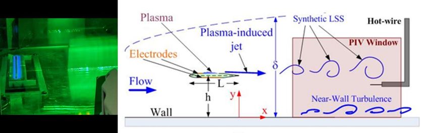
PIV Experiment
 The PIV experimental setup is shown schematically in Figure 2. Planar PIV was used to
 measure the streamwise and wall-normal velocity fields downstream of the plasma actuator along
 the mid-span plane of the test section. The flow was seeded with DEHS particles (diameter <
 1 ) and illuminated with a 532nm laser sheet. The laser sheet was expanded through the top of
 the test section had a nominal thickness of 1 (0.03 or 20 + ) at the boundary layer
 development plate surface. Images were captured with a Phantom v1840 high-speed camera at a
 resolution of 1280 × 720 2 . The camera was fitted with an AF NIKKOR 50mm f/1.4D lens
 attached to a 2x telephoto converter. The lens was positioned perpendicular to the measurement
 plane, just outside of the test section, resulting in a 70 × 40 (2 × 1.2 or
 1400 + × 800 + ) streamwise by wall normal field of view (FOV). The overlap between FOVs
 was 17 (0.5 or 340 + ) in the streamwise direction. Using this spacing, images were
Downloaded by Stanislav Gordeyev on December 30, 2021 | http://arc.aiaa.org | DOI: 10.2514/6.2022-0053

 acquired at 6 streamwise locations where the FOVs were centered at = 1, 2, 3.5, 5, 6.5, 8 .
 The frame rate of the camera was 12 ( = 60 ∞ / or ∆ + = 0.5 or 150 ). The image
 acquisition and plasma forcing were triggered simultaneously so that the images collected were
 phase-locked to the plasma actuation cycle. The images were acquired using the Phantom Camera
 Control software and the images were processed using LaVision’s DaVis software. The vector
 fields were calculated using a single-pass correlation method with an interrogation window size of
 64 × 64 2 with no overlap between windows. The resulting spatial resolution of the resulting
 vector fields in the wall-normal direction was 0.09 or 60 + .

 Figure 2. Schematic of experimental set-up with picture of PIV laser sheet downstream of
 ALSSA device.

 III. Data Reduction
 The data reduction for these experiments started with properly converting the measured hot-
 wire probe voltages and PIV images into velocities using the methods described earlier. After the
 time series of velocities were obtained, the time mean, U, and root mean square (RMS) of the
 velocity, were calculated at every point using standard methods. Since the actuator
 introduced periodic forcing into the flow, it is convenient to phase-lock the results to the actuation
 frequency. To do so, a triple phase-locked Reynolds decomposition of the velocity was considered,
 as shown in Equation 1,
 ( , , ) = ( , ) + ̃( , , ) + ′( , , , ) (1)

 5

where is the instantaneous velocity, U is the time mean component of velocity, ̃ is a phase
 dependent or modal velocity component, ′ is a residual fluctuating turbulent component, φ is the
 phase, defined by the relationship in Equation 2, and n is the number of realizations as described
 below.
 
 = ( + ) (2)
 2 
 Here is a time in the ℎ realization or cycle, which is related to the phase angle, φ, by the period
 of the forcing repetition cycle, = 1/ . The output of the function generator was used to ensure
 the hot-wire data was phase locked with the forcing of the plasma. These n realizations were then
 ensemble averaged to determine the modal component of velocity as a function of the phase angle.
 The remaining fluctuating component of the velocity, ′ was used to quantify an ensemble-
Downloaded by Stanislav Gordeyev on December 30, 2021 | http://arc.aiaa.org | DOI: 10.2514/6.2022-0053

 averaged RMS of the residual fluctuating turbulence.
 1
 ′
 ( , , ) = (⟨[ ′ ( , , , )]2 ⟩ )2 (3)

 ′ ′
 ( , ) = ′
 ( , ) − ⟨ ( , )⟩ 
 (4)

 Here the square brackets denote ensemble averaging over all realizations. Later we will refer to
 this quantity as a residual turbulence level. A so called ϕ-coefficient which was introduced in [8]
 and is shown in Equation 4. This so-called modulation coefficient relates changes in the modal
 velocity component to those in the residual fluctuating turbulence that was described above. The
 modulation coefficient is essentially a quantification of the phase between the modal velocity and
 residual turbulence fluctuations.
 ′
 ⟨ ̃( , , ) ( , , )⟩ 
 Φ( , ) =
 (5)
 √⟨ ̃( , , )2 ⟩ √⟨ 
 ′ ( , , )2 ⟩ 

 IV. Hot-Wire Results
 In earlier hot-wire experiments [10] the forcing frequency of the actuator was set to 50 Hz
 (0.23 ∞ / ). This frequency was used initially because it produces synthetic large-scale motions
 that match the size of naturally occurring large-scale structures in higher Reynolds number
 canonical boundary layers, as shown in Equation 5. The streamwise wavelength of coherent large-
 scale motions in canonical boundary layers were estimated to be between = 3 − 6 based on
 measurements of higher Reynolds number TBLs [1].

 ∞ / = (6)

 It was suspected that because this forcing frequency was based on outer variable scaling
 there may exist other forcing frequencies, potentially scaled by inner variables, which would lead
 to a preferred response in the near wall region. To test this hypothesis, the hot-wire probe was
 placed in the near wall region at + = 20 and the frequency of the plasma forcing cycle was varied

 6

from 20 – 200 . The modal velocity and residual turbulence were measured so that the
 modulation coefficient near the wall could be computed for each frequency. The results of this
 study are presented in detail in references [12] [11]. The highest modulation coefficient was
 observed for a band of frequencies centered around 80 Hz which is closely related to characteristic
 near-wall frequencies. Further experimentation with a forcing frequency of 80 Hz revealed that
 the modulation coefficient across the entire log-region and in the near-wall region was higher with
 the increased forcing frequency. Based on these results the forcing frequency was increased to 80
 Hz for all the experiments discussed here.
 Along with the forcing frequency, it was expected that variations in the wall normal position
 of the actuator would change the modulating influence of the plasma forcing in the near-wall
 region. A wall normal position of ℎ = 0.6 was chosen in earlier studies based on observations of
 near-wall turbulence modulation in [8] where this wall-normal location was shown to be an
Downloaded by Stanislav Gordeyev on December 30, 2021 | http://arc.aiaa.org | DOI: 10.2514/6.2022-0053

 effective location for forcing. A second wall normal position of ℎ = 0.3 which is just above the
 log region, was considered because it is much closer to the location of the naturally occurring
 coherent spanwise oriented large-scale structures. At this actuator location, the modulation
 coefficient was not changed significantly, but the turbulence intensity and skewness near the wall
 were decreased suggesting there was a stronger interaction between the large and small scales
 when the forcing was moved closer to the wall. The full results of this study are presented in [12].
 Because of these results the actuator height above the plate was decreased to ℎ = 0.3 for the
 experiments discussed here.
 Studies of the spanwise variation in forcing across the actuator were also conducted to ensure
 the actuator produced two-dimensional motions across an appropriately large spanwise region.
 The full results of this study are also presented in [12]. It was found that within one boundary layer
 thickness of either end of the plate, there are significant three-dimensional motions associated with
 the finite length of the actuator plate and plasma electrodes. To simulate natural large-scale
 structures more appropriately, the region of two-dimensional forcing should be on the order of 6 
 [1]. Based on these observations the plate was widened to = 8 . The plate was also shortened
 in the streamwise direction to reduce the wake effect from the actuator plate itself, making the
 effect of the plasma forcing more distinguishable.
 With the updated actuator design, a set of experiments were conducted in the same manner as
 the preliminary experiments presented in [12]. The canonical boundary layer was measured with
 the hot-wire at each measurement location to establish a baseline before introducing the physical
 actuator plate or applying plasma forcing. The premultiplied streamwise energy spectra for a single
 measurement location is presented in Figure 3(a). The near-wall or inner energy peak aligns well
 with the expected location of + = 15, + = 1000 marked by the white cross. At the relatively
 low Reynolds number of = 690 in this experiment, there is no discernable energetic coherent
 large-scale structure that normally shows up as an outer peak in the premultiplied spectra [1].
 Large-scale motions are still present in the boundary layer but result in a diffuse lobe in the spectra
 extending away from the wall. This lobe is consistent with the predicted location that natural LSS
 would exist as indicated by the open circle in Figure 3(a). The streamwise wavelength of the
 natural coherent LSS has been reported on the order of 3 − 6 [16] [1], and was chosen to
 nominally be = 4 for this analysis. In addition to the quantitative agreement of the

 7

premultiplied spectra, there is also qualitative agreement with other experiments at similar
 Reynolds numbers [1].
 The canonical mean velocity profile and turbulence intensity profiles can be seen in Figure
 3(b). There is a well-defined log-linear region in the mean velocity profile from + = 40 − 200
 and near the wall the velocity profile approaches the linear scaling of the viscous sublayer, though
 the measurements do not extend into the sublayer in this case. The peak in the turbulence intensity
 occurs near + = 16 and has an error in normalized amplitude of approximately 20% [15].
 The actuator was subsequently introduced, and velocity data were collected for the plasma off
 case, to quantify the passive effect of the actuator plate, and plasma on case. The premultiplied
 spectra for both cases can be seen in Figure 4. In Figure 4(b) the coherent structure produced by
 the plasma forcing can be seen as a peak in the premultiplied spectra in the outer region. With the
 improvements to the actuator forcing frequency and wall-normal actuator location, the synthetic
Downloaded by Stanislav Gordeyev on December 30, 2021 | http://arc.aiaa.org | DOI: 10.2514/6.2022-0053

 structure signature is near the predicted naturally occurring structure indicated by the black circle.
 The mean velocity, turbulence intensity and skewness profiles were not significantly altered by
 the changes in actuator properties. The results can be found in previous studies where the plasma
 on and off cases were analyzed statistically [12].

 (a) (b)

 Figure 3. (a) Premultiplied streamwise energy spectra for the canonical
 boundary layer at = 5 . Cross marks inner peak ( + = 15, + =
 1/2
 1000). Open circle marks predicted outer peak ( + = 3.9 , + ≈
 3 ) for = 690. (b) Mean velocity and turbulence intensity profiles.

 To further characterize the isolated effect of the plasma forcing, measurements for the
 actuator plate alone (plasma off case) were subtracted from the cases where the plasma forcing
 was active. The difference in premultiplied spectra between the plasma on and off cases at two
 different streamwise locations can be seen in Figure 5. There is a clear contribution to the energy
 spectra at the wavelengths associated with the plasma forcing frequency across the boundary layer.
 The strongest contribution at the location x = 1.5 is at the actuator height as shown in Figure 5(a),
 but there is an additional elongated peak that extends though the log region and into the near wall
 region. This signature of the large-scale motions from the actuator is similar to the signature of

 8

dynamic roughness perturbations presented in [2] which originate within the log-region closer to
 the wall. At the farther downstream location of x = 5, the peak in energy in Figure 5(b) has shifted
 and is more concentrated within the log-region. There are also changes in the near wall energy
 peak at both downstream locations which is an indication that the actuator-induced large-scale
 motions are interacting with the near-wall small-scale structures. Like the results of [2], the
 discrepancies in the pre-multiplied spectra seen here show the receptivity of the TBL to large-scale
 perturbations. In this case, energy introduced through the synthetic large-scale motions in the outer
 layer is also changing the organization of structures near the wall through some outer-inner
 interaction mechanism.
Downloaded by Stanislav Gordeyev on December 30, 2021 | http://arc.aiaa.org | DOI: 10.2514/6.2022-0053

 Figure 4. (a) Plasma off and (b) plasma on premultiplied spectra at = 1.5 . ℎ+ = 200. Cross
 marks inner peak ( + = 15, + = 1000). Open circle marks predicted outer peak ( + =
 1/2
 3.9 , +
 ≈ 3 ).

 (a) (b)

 Figure 5. Discrepancy between plasma on, = 80 , and plasma off premultiplied spectra at
 (a) = 1.5 and (b) = 5 . ℎ+ = 200. Cross marks inner peak ( + = 15, + = 1000). Open
 1/2
 circle marks predicted outer peak ( + = 3.9 , + ≈ 3 ).

 The phase-locking method described earlier was implemented to analyze the effect on the
 near wall turbulence associated with the LSS introduced by the plasma forcing. To start, maps of
 the modal velocity and residual turbulence were computed for each streamwise measurement

 9

location. The results of the phase-locked analysis of the hot-wire data is shown in Figure 6 and
 Figure 7. The modal velocity results for x = 1.5 and 3 are shown in Figure 6(a,b) and Figure
 7(a,b) presents the results for x = 5 and 8. At each streamwise location, there is a strong modal
 velocity signature at the actuator location attributed to the large-scale motions produced by the
 actuator convecting downstream. Below the actuator there is also a significant modal velocity
 signature that extends towards the wall. Downstream the modal fluctuations near the wall lag
 slightly behind the phase of the signature in the outer region. As seen earlier when inspecting the
 premultiplied spectra, as the large-scale motions produced by the actuator are convecting
 downstream the strongest modal fluctuations are spreading and moving downwards into the log
 region.
 The residual turbulence fluctuations at the locations x = 1.5 and 3 are shown in Figure
 6(c,d) and locations x = 5 and 8 are shown in Figure 7(c,d). At farther downstream locations,
Downloaded by Stanislav Gordeyev on December 30, 2021 | http://arc.aiaa.org | DOI: 10.2514/6.2022-0053

 see Figure 6(c,d) there is a strong residual turbulence signature at the actuator height due to the
 plasma forcing. By analyzing the 2 criteria, related to the vorticity, it was found that the strong
 positive fluctuations in residual turbulence are convecting with the center of the synthetic large-
 scale structures produced by the actuator. There is also an important region of residual turbulence
 fluctuation which occurs directly below the convecting LSS and extends towards the wall. The
 positive fluctuations in this region are aligned with the positive fluctuations at the actuator height
 meaning they occur directly below the convecting LSS. Within this region, near the wall the small-
 scale turbulent structures have been modulated by the large-scale motions introduced by the
 actuator. Moving downstream the intensity, shape, and inclination of this region of modulated
 turbulence are all changing as the synthetic large-scale structures convect downstream. These
 developments will be discussed in more detail later.

 10

Downloaded by Stanislav Gordeyev on December 30, 2021 | http://arc.aiaa.org | DOI: 10.2514/6.2022-0053

 Figure 6. (a,b) Phase maps of modal velocity (c,d) phase maps of residual turbulence (e,f)
 modulation function Ф. (a,c,e) = 1.5 (b,d,f) = 3 . ℎ+ = 200, = 80 . The horizontal
 dashed line represents the actuator location.

 11

Downloaded by Stanislav Gordeyev on December 30, 2021 | http://arc.aiaa.org | DOI: 10.2514/6.2022-0053

 Figure 7. (a,b) Phase maps of modal velocity (c,d) phase maps of residual turbulence (e,f)
 modulation function Ф. (a,c,e) = 5 (b,d,f) = 8 . ℎ+ = 200, = 80 . The horizontal
 dashed line represents the actuator location.

 12

The modulation coefficient described earlier is presented in Figure 6(e,f) and Figure 7(e,f)
 in order to characterize the development of the phase relationship between the modal velocity and
 the residual turbulence fluctuations at various streamwise locations. At the downstream location
 nearest the actuator, Figure 6(e), the modulation coefficient is nearly one at the wall and decreases
 moving away from the wall until it reaches zero at the geometric center of the log region ( + =
 100). By the farthest downstream measurement station, shown in Figure 7(f), the modulation
 coefficient at the wall has reduced to zero, but throughout the log region the modulation coefficient
 is nearly one. This shift in the modulation coefficient shows that the boundary layer is gradually
 adjusting to the presence of the synthetic LSS.
 To visualize the streamwise development of the fluctuations in modal velocity and residual
 turbulence it is possible to reconstruct the hot-wire results along a pseudo-spatial streamwise
 coordinate. The modal velocity component just above the actuator is well defined and continuous
Downloaded by Stanislav Gordeyev on December 30, 2021 | http://arc.aiaa.org | DOI: 10.2514/6.2022-0053

 between downstream locations. By looking at the periodic signature of the modal velocity, the
 phase of the measurement can be transformed into a spatial coordinate using an appropriate
 convective velocity, as shown in Equation 7. The convective velocity parameter was adjusted until
 the modal velocity component measured at + = 300 was continuous between each streamwise
 measurement locations as expected.

 1
 = − 2 (7)
 
 Applying this convective velocity and Taylor’s frozen field hypothesis, the phase of
 previous measurements was converted into a pseudo spatial streamwise coordinate at each
 measurement location. The convective velocity parameter changes with both wall-normal and
 streamwise position. A pseudo-spatial reconstruction of the residual turbulence for the whole flow
 field downstream of the actuator can be seen in Figure 8. The reconstruction was limited to a single
 period of measurement to avoid violating the assumptions that the flow can be considered frozen.
 The accuracy of using this reconstruction method will be discussed later.

 Figure 8. Pseudo spatial map of residual turbulence. ℎ = 0.3 , = 80 .

 Looking at Figure 8, the spatial development of the regions of modulated residual turbulence
 near the wall and at the actuator location is clarified. At any streamwise location where the
 synthetic large-scale structures are convecting past, strong positive fluctuation is present around
 and above = 0.3 . But there is also a region of positive fluctuation in the log region and near
 the wall. There are clear differences in the extent and inclination of the regions of modulated
 turbulence with downstream distance. Specifically, the inclination of these regions with respect to

 13

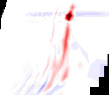
the wall are changing and becoming closer to the inclination of structures measured in higher
 Reynolds number canonical boundary layers [2].

 V. PIV Results
 After the hot-wire results were established, planar PIV was used to make spatially resolved,
 and time resolved, measurements of the streamwise and wall-normal velocity components over the
 same field downstream of the actuator. By directly measuring these quantities in space and time,
 the analysis of the interaction between the synthetic large-scales and modulated near-wall
 structures can be improved. Here the preliminary PIV results will be compared to the hot-wire
 measurements presented earlier and the spatially resolved numerical simulation presented in [13].
 The mean velocity and turbulence intensity profiles for a single x-location are shown in Figure 9.
 The mean velocity results match the hot-wire results well except for the point nearest the wall. The
Downloaded by Stanislav Gordeyev on December 30, 2021 | http://arc.aiaa.org | DOI: 10.2514/6.2022-0053

 spatial averaging effect of the large PIV interrogation window size contributes to the discrepancy.
 The measurements in this region are also highly sensitive to small errors in the wall-normal
 position. It should also be noted that for the PIV measurement there are only a few points in the
 log region of the boundary layer. Because of the importance of this region, it would be beneficial
 to increase the spatial resolution of the measurement in future experiments. In the turbulence
 intensity profile these errors are more exaggerated. Just as the hot-wire length caused a loss of
 measured turbulence intensity the low spatial resolution of the PIV measurements will cause an
 even greater loss of measured turbulence intensity, as shown by the underestimate of the PIV
 profile compared to the hot-wire. However, this figure demonstrates that the PIV measurements
 are statistically consistent with the hot-wire results, but they present new experimental errors that
 must be quantified or corrected.

 (a) (b)

 Figure 9. Comparison of (a) mean velocity and (b) turbulence intensity
 profiles for the hot-wire and PIV measurements of plasma on case.
 = 5 , ℎ = 0.3 , = 80 .

 In addition to statistical quantities, the modal components of both the streamwise and wall-
 normal velocities have been computed and are presented in Figure 10 and Figure 11 respectively.
 The hot-wire results have been reconstructed in the pseudo-spatial coordinate for a more direct

 14

comparison. The wall-normal velocity was not directly measured by the hot wire but was estimated
 using the phase-locked velocity signal. After converting the phase-locked velocity signal into the
 pseudo spatial coordinate, as described in Equation 7, the spatial derivatives were estimated
 numerically, and the continuity relationship was used to determine the wall-normal velocity
 component. This resulted in an estimation of the pseudo-spatial wall-normal modal velocity for
 each measurement location.
 The streamwise component modal velocity fields are shown in Figure 10. From the actuator
 trailing edge up to = 5 , there is a strong agreement between the hot-wire reconstruction, the
 PIV measurement, and the numerical results, presented in [13]. The phase of the periodic
 fluctuations matches well across the entire boundary layer height and the magnitude of the
 fluctuations are nearly identical. Farther downstream there are some discrepancies between the
 experimental and numerical results. The numerical results show very periodic fluctuations, while
Downloaded by Stanislav Gordeyev on December 30, 2021 | http://arc.aiaa.org | DOI: 10.2514/6.2022-0053

 the experimental results show regions of less regular fluctuation around = 6 as the synthetic
 large-scale motions diffuse across the boundary layer. There is a gap in the hot-wire data around
 this location as well as a phase mismatch near the wall starting at a streamwise location of = 7 .
 This is a result of the pseudo-spatial reconstruction method where measurements at a single point
 are used to estimate the behavior upstream. Looking at the PIV results, the periodic behavior at
 = 8 does not match well with the less simple behavior seen between = 5 − 6 so the
 assumptions necessary for reconstruction may only be valid for a smaller region upstream of the
 measurement location. The PIV and numerical results have good agreement in the phase and
 intensity of the fluctuations near the wall at the farther downstream locations. The PIV
 measurements are not as spatially resolved near the wall as the hot-wire and numerical results, but
 experiments are currently underway to resolve this region and specifically the turbulence
 fluctuations. The wall-normal modal velocity fields are shown in Figure 11. The same phase
 mismatch is seen between the PIV and hot-wire as expected. Outside of this region, the phase and
 intensity of the wall-normal modal velocity fluctuations match well between each method.
 In addition to the modal velocity components, the PIV measurements can be used to
 calculate the residual turbulence component. A comparison of the residual turbulence results can
 be seen in Figure 12. Due to the spatial resolution of the PIV measurements, we are not yet able to
 make comparisons in the region below = 0.05 or above = 0.8 . In the region between =
 0.1 − 0.4 there is a clear region positive fluctuation which has been referred to as the region of
 modulated turbulence. This region also appears in the PIV measurement at the same phase and
 over the same wall-normal extent. In the region between = 0.4 − 0.6 there is again agreement
 between the hot-wire and PIV results, but the PIV measurements show a slightly higher amplitude
 than the hot-wire measurements. Above = 0.6 there appears to be a slight phase shift between
 the PIV and hot-wire results. Without having the PIV results for higher wall-normal locations it is
 difficult to determine if this shift is an error in the phase or an error in the amplitude of the tail of
 the fluctuations the extend down from the outer region which is seen faintly in the hot-wire results.

 15

(a)
Downloaded by Stanislav Gordeyev on December 30, 2021 | http://arc.aiaa.org | DOI: 10.2514/6.2022-0053

 (b)

 (c)

 Figure 10. Streamwise modal velocity component measured by (a) hot-wire (b) PIV and (c)
 simulated numerically. ℎ = 0.3 , = 80 .

 16

(a)
Downloaded by Stanislav Gordeyev on December 30, 2021 | http://arc.aiaa.org | DOI: 10.2514/6.2022-0053

 (b)

 (c)

 Figure 11. Wall-normal modal velocity component (a) estimated using
 hot-wire data (b) measured by PIV and (c) simulated numerically. ℎ =
 0.3 , = 80 .

 Figure 12. Phase plot of residual turbulence at = 5 measured by (a)
 hot-wire and (b) PIV. ℎ = 0.3 , = 80 .

 17

VI. Conclusions a Future Work

 The plasma-based actuator design was updated based on previous experimental results [12]
 and analyzed using a single hot-wire probe. The results presented here for the improved actuator
 were found to be statistically consistent with the original results. Using a modal decomposition, it
 was found that the synthetic LSS produced by the improved actuator still has a strong modulating
 effect on the turbulence near the wall. This modulating effect is similar to the effects described in
 [3] where large-scale motions were introduced to the TBL at the wall. In the current study the
 region of turbulence modulated by the presence of the synthetic LSS changes in shape and extent
 as the LSS convect downstream. The changes demonstrate the receptivity of the TBL to large-
 scale forcing as the TBL adjusts to the presence of a synthetic LSS. Planar PIV was used to
 measure the spatially and temporally resolved two-dimensional velocity field downstream of the
Downloaded by Stanislav Gordeyev on December 30, 2021 | http://arc.aiaa.org | DOI: 10.2514/6.2022-0053

 actuator. The PIV measurements were found to be statistically consistent with the hot-wire
 measurements. It was also shown that through modal decomposition the PIV measurements could
 capture the dynamics of the synthetic LSS consistent with both the hot-wire results and spatially
 resolved numerical simulations [13]. The PIV measurements also captured some of the turbulence
 modulating effect but were limited by spatial resolution in the current experiments.
 The planar PIV measurements are ongoing. Having spatially and temporally resolved
 measurements of the two-dimensional field will allow for improved analysis of the correlation
 between the synthetic LSS and the modulated near-wall turbulence. These measurements will
 supplement and provide additional support to the conclusions from the original hot-wire
 experiments. The immediate goal with the planar PIV is to improve the spatial resolution of the
 PIV field to better capture turbulence fluctuations. Planar PIV will be used to measure the entire
 field downstream of the actuator as well as across different spanwise planes for a more complete
 measurement of the effect of the synthetic LSS. The measurement plane can also be made normal
 to the wall in order to measure a spanwise-streamwise field near the wall to complete the
 characterization of the effect of the outer-inner interaction mechanism.

 References

 [1] N. Hutchins and I. Marusic, "Large-scale influences in near-wall turbulence," Phil. Trans.
 R. Soc. A, vol. 365, pp. 647-664, 2007.
 [2] S. Duvuuri and B. McKeon, "Phase relations in a forced turbulent boundary layer:
 implications for modelling in high Reynolds number wall turbulence," Phil. Trans. A, vol.
 375, 2017.
 [3] S. Duvuuri and B. McKeon, "Triadic scale interactions in a turbulent boundary layer," J.
 Fluid Mech., vol. 767, p. R4, 2015.
 [4] S. K. Robinson, "Coherent Motions in the Turbulent Boundary Layer," Ann. Rev. Fluid
 Mech., vol. 23, pp. 601-639, 1991.
 [5] C. M. de Silva, N. Hutchins and I. Marusic, "Uniform momentum zones in turbulent
 boundary layers," J. Fluid Mech., vol. 786, pp. 309-331, 2016.

 18

[6] R. J. Adrian, C. D. Meinhart and C. D. Tomkins, "Vortex organization in the outer region of
 the turbulent boundary layer," J. Fluid Mech., vol. 422, pp. 1-53, 2000.
 [7] D. E. Coles and E. A. Hirst, "Comutation of Turbulent Boundary Layers: Compiled Data,"
 in AFOSR-IFP, Stanford University, 1968.
 [8] P. Ranade, S. Duvuuri, B. McKeon, S. Gordeyev, K. Christensen and E. J. Jumper,
 "Turbulence Amplitude Amplification in an Externally Forced, Subsonic Turbulent
 Boundary Layer," AIAA Journal, vol. 57, pp. 3838-3850, 2019.
 [9] Z. Tang and N. Jiang, "The effect of a synthetic input on small-scale intermittent bursting
 events in near-wall turulence," Phys. Fluids, vol. 31, 2019.
 [10] M. Lozier, S. Midya, F. Thomas and S. Gordeyev, "Experimental Studies of Boundary Layer
 Dynamics Using Active Flow Control of Large-Scale Structures," in TSPF-11,
Downloaded by Stanislav Gordeyev on December 30, 2021 | http://arc.aiaa.org | DOI: 10.2514/6.2022-0053

 Southhampton, UK, 2019.
 [11] M. Lozier, F. Thomas and S. Gordeyev, "Streamwise Evolution of Turbulent Boundary
 Layer Response to Active Control Actuator," in AIAA Scitech, 2020.
 [12] M. Lozier, F. O. Thomas and S. Gordeyev, "Turbulent Boundary Layer Repsosne to Active
 Control Plasma Actuator," in AIAA Scitech, 2021.
 [13] C. Lui, I. Guzman, M. Lozier, F. Thomas, S. Gordeyev and D. Gayme, "Spatial input–output
 analysis of large-scale structures in actuated turbulent boundary layers," AIAA Journal,
 2021*.
 [14] F. O. Thomas, T. C. Corke, M. Iqbal, A. Kozlov and D. Shatzman, "Optimization of SDBD
 Plasma Actuators for Active Aerodynamic Flow Control," AIAA Journal, vol. 47, pp. 2169-
 2178, 2009.
 [15] N. Huthcins, T. B. Nickels, I. Mausic and M. S. Chong, "Hot-wire spatial resolution issues
 in wall-bounded turbulence," J. Fluid Mech., vol. 635, pp. 103-136, 2009.
 [16] M. Guala, S. E. Hommema and R. J. Adrian, "Large-scale and very large-scale motions in
 turbulent pipe flow," J. Fluid Mech., vol. 554, pp. 521-542, 2006.
 [17] T. S. Luchik and W. G. Tiederman, "Timescale and structure of ejections and busts in
 turbulent channel flows," J. Fluid Mech., vol. 174, pp. 529-552, 1987.
 [18] J. Jeong and F. Hussain, "On the identification of a vortex," J. Fluid Mech., vol. 285, pp. 69-
 94, 1995.
 [19] M. Wicks and F. O. Thomas, "Effect of Relative Humidity on Dielectic Barrier Discharge
 Plasma Actuator Body Force," AIAA Journal, vol. 53, 2015.
 [20] R. Mathis, N. Hutchins and I. Marusic, "Large-Scale Amplitude Modulation of the Small-
 Scale Sturcutres in Turbulent Boundary Layers," J. Fluid Mech., vol. 658, pp. 311-336, 2009.

 19