PORTABLE 512 MEMS-MICROPHONE-ARRAY FOR 3D-INTENSITY- AND BEAMFORMING-MEASUREMENTS USING AN FPGA BASED DATA-ACQUISITION-SYSTEM - BEBEC 2020
←
→
Page content transcription
If your browser does not render page correctly, please read the page content below
BeBeC-2020-D27

 Portable 512 MEMS-Microphone-Array for 3D-Intensity- and
     Beamforming-Measurements using an FPGA based
                 Data-Acquisition-System

  Daniel Ernst1 , Reinhard Geisler1 , Tobias Kleindienst1 , Thomas Ahlefeldt1 , Carsten Spehr1
     1 DLR   Institute of Aerodynamics and Flow Technology, Experimental Methods Department
                               Bunsenstr. 10, 37073 Göttingen, Germany

                                              Abstract
         In this paper a portable MEMS-Microphone-Array with integrated Data-Acquisition-
      System is presented. 512 digital MEMS-Microphones are located in a rectangular box of
      17 x 15 x 20 cm. The microphone positions are chosen for sound intensity measurements,
      but are capable of beamforming as well. Depending on the frequency, these microphones
      can be used as an array of hundreds of 3D - intensity probes. The acoustic velocity is
      estimated using a high order three dimensional finite difference stencil to overcome the
      upper frequency limit of common pp-intensity probes. At low frequencies, pairs with larger
      spacing are used to reduce the requirement of accurate phase match of the microphone
      sensors. Additionally a procedure is shown for amplitude and phase calibration of MEMS-
      Sensors.
      All microphone data is collected by an FPGA and send via the UDP-Protocol to any host
      system for beamforming and intensity calculations in real time or for storing the data to
      disk.

1 INTRODUCTION

Handheld acoustic arrays are commercially available containing up to 128 microphones. These
microphone arrays can be used for beamforming, acoustic intensity measurements or nearfield
holography. In order to calculate the acoustic intensity, all these arrays have in common that
the microphones are arranged in one or two planes which are placed in parallel to a acoustic
radiating surface. Predefined knowledge of the direction of the acoustic intensity is needed.
Another common problem is the position tracking of the microphone array itself in the three di-
mensional space. Camera based systems are available but require the microphone array to stay
in the field of view of a stationary camera. The third limitation is the time required to perform

                                                  1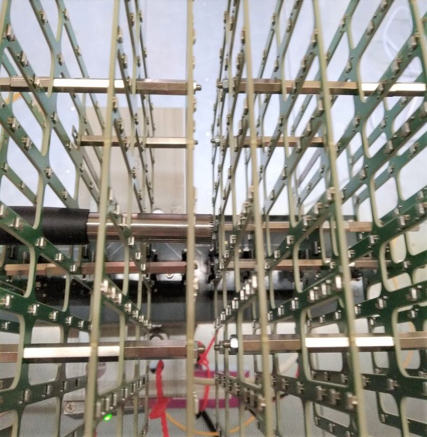
8th Berlin Beamforming Conference 2020                                                 Ernst et al.

accurate sound intensity measurement. A diffuse sound field may need treatment with acoustic
absorbing material and a high spatial resolution requires a long measurement period.
In complex environments like an aircraft cabin under flight conditions the direction of the sound
intensity is unknown, stationary tracking cameras are unavailable and a reduction of measur-
ment time is desirable. Therefor a 3D-intensity probe combined with an optical tracking system
based on Intel Realsense Cameras was designed to treat these issues. The low weight, small
size and low power consumption led to the choice of using MEMS microphones.
There are several studies on using MEMS microphones as an array for example fan mea-
surements [1], beamforming [9], real-time speech acquisition [3] or boundary layer measure-
ments [13]. Most of the digital implementations of MEMS arrays are using FPGAs (Field
Programmable Gate Arrays) for the data processing due to their flexibility in programming,
scalability regarding sensor count and power consumption.
It is possible to perform a primary calibration of MEMS microphones using the pressure reci-
procity [11] or a novel method using photon correlation spectroscopy [10]. Both methods are
complex to handle.
There are two options for secondary calibration using a reference microphone. The first method
assures that the reference microphone is placed in a tube or cavity smaller than the acoustic
wavelength [13] [9] and the second method assumes free field conditions and the device under
test and the reference microphone are placed close to each other [8]. For low frequencies the
first method is applicable and for high frequencies the second one. In this paper both types are
performed.
Kotus et. al. [6] performend the calibration of a MEMS based intensity probe in the free field
without a calibration of individual frequency response functions.
The next step in measuring the sound intensity is the calculation of the acoustic particle velocity
[2]. A PP-probe uses the 2-point finite difference stencil between the microphones to estimate
the spatial derivation of the acoustic pressure field.
Wiederhold et. al. [14] and Lawrence et. al. [7] extended these formulation to a high order
finite difference scheme in three dimensions. We will use these methods to estimate the acoustic
intensity vector in section 2.2.

2 THEORY AND METHODS

2.1 Hardware Implementation

There are 512 MEMS Microphones of the Type ICS 52000 with an 24-bit integrated AD-
conversion distributed over 8 identical PCBs (printed circuit boards). Each PCB contains there-
for 64 microphones. The spacing of the PCBs is non-equidistant to provide small spacings for
high frequencies and large spacings for low frequencies.
All digital microphone data is time synchronized collected at a sampling frequency of 48 kHz
from an FPGA (Xilinx Artix 7) and transmitted to a GigEx-Ethnernet ASIC which implements
a full network stack and sends one UDP packet per sample to a host laptop to collect all data.
The resulting datarate is ≈ 80 MB/s.
The overall power consumption of the microphone array and the FPGA is approximately
1.8 A · 3.3 V ≈ 5 W. Thus it is possible to use a LiPo battery pack with 56.5 Wh for hand-
held measurements of several hours.

                                                2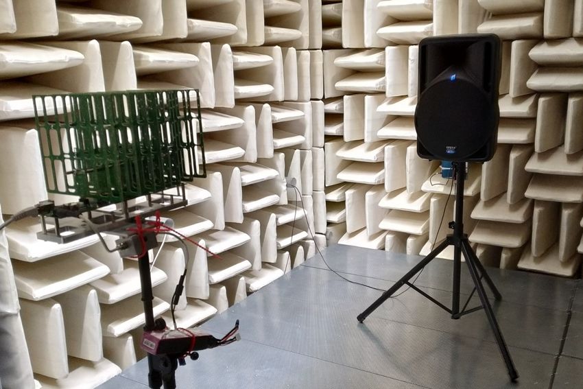
8th Berlin Beamforming Conference 2020 Ernst et al.
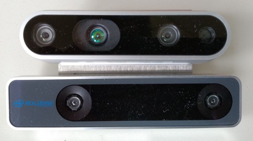
Two Intel Realsense Cameras (T265 and D435) are mounted below the microphone array and
the pose and depth information is collected from the same host laptop. The pose, containing
translation and rotation, is sampled at 200 Hz and the depth images at 30 Hz. The synchroniza-
tion of the two cameras and the microphone array is done with the hardware time stamps.
2.2 Sound Intensity
According to Fahy [2] the mean sound intensity I in the frequency domain is the cross spectra
of the acoustic pressure P and velocity U
1
I = Re(P · U∗ ) (1)
2
and by combining equation 1 with the fluid momentum equation in the frequency domain
j
U= ∇P (2)
ωρ0
results in
1
I= Re( jP · ∇P∗ ) (3)
2ωρ0
The acoustic pressure P and its spatial gradient ∇P is estimated using a multidimensional
Taylor expansion at every microphone position. A system of linear equation is set up by sum-
ming up the expansions and set all the terms proportional to a specific exponent to zero. See
Lawrence et. al. [7] for further details.
The overall approximation order M is defined as
M = Mx My Mz (4)
where Mx , My and Mz are the orders in the different spatial directions.
We denote P̂ ∈ RN as the complex pressure per microphone in the frequency domain, N as the
number of microphones, y ∈ R3 as the position where the acoustic intensity is calculated and
xn ∈ R3 as the n-th microphone position.
With these assumptions four systems of linear equations are formed:
w = A−1 b, wx = A−1 bx , wy = A−1 by , wz = A−1 bz (5)
where
(y1 − xn,1 )n1 (y2 − xn,2 )n2 (y3 − xn,3 )n3
[A]n1 +n2 M1 +M1 M2 n3 ,n = (6)
nx !ny !nz !
and
[b]m = δ (m) (7)
[bx ]m = δ (m − 1), [by ]m = δ (m − 1 − M1 ), [bz ]m = δ (m − 1 − M1 M2 ) (8)
.
3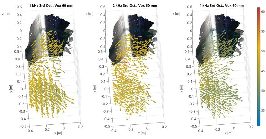
8th Berlin Beamforming Conference 2020                                                 Ernst et al.

  The acoustic pressure and its spatial derivatives at the point y are then estimated as follows:
                                   ∂ P∗            ∂ P∗            ∂ P∗
                      P ≈ wT P̂,        ≈ P̂∗ wx ,      ≈ P̂∗ wy ,      ≈ P̂∗ wz               (9)
                                    ∂x              ∂y              ∂z
Using equation 9 and 3 the acoustic intensity is calculated as follows:

                           ωρ0 Ix ≈ Re( jwT P̂P̂∗ wx ) = Re( jwT Cwx )                        (10)
                           ωρ0 Iy ≈ Re( jwT P̂P̂∗ wy ) = Re( jwT Cwy )                        (11)
                           ωρ0 Iz ≈ Re( jwT P̂P̂∗ wz ) = Re( jwT Cwz )                        (12)
                                                                                              (13)

   Here the cross spectral matrix C ∈ CN,N is introduced as known from classical beamforming
and the presented approach can be interpreted as steering on the acoustic intensity. An advan-
tage regarding processing speed compared to classical beamforming is that the steering vectors
are independent of the frequency.

2.3 Position tracking and 3D-Model of the environment

If the PP512-MEMS Array is used as a handheld device a position tracking system can be
used. This system contains two Intel Realsense cameras that are solidly attached to the micro-
phone array. The Intel Realsense T265 camera estimates the position and orientation at 200 Hz
sampling frequency and a three dimensional point cloud is given by the Intel Realsense D435
camera at 30 Hz sampling frequency. This point cloud is then rotated and translated according
to the global position retrieved by the pose camera (T265). By using the ”open3d” [15] python
package voxel downsampling is performed on the resulting point cloud. In addition the method
”poisson surface reconstruction” of the ”open3d” [15] package is used to create triangle mesh
for further visualizations.

3 MEASUREMENTS AND RESULTS

In this paper two different calibration procedures are carried out: cavitiy and freefield calibra-
tion. Both methods are second order calibrations. That means that a device under test (DUT,
here the MEMS microphone) is compared to a reference microphone.

3.1 Cavity Calibration

In order to do a cavity calibration, one has to assure that the DUT and the reference microphone
are close to each other in a cavity with lengths much smaller than the wavelength.
Here a phase calibrator 51AB from G.R.A.S. is used to calibrate the amplitude and phase
between two different MEMS microphones of the type ICS 52000. A reference microphone
(G.R.A.S. 1/2”) is placed in one side of the calibrator and a cylinder made of aluminium (di-
ameter 1/2”, height 15 mm) with a 5 mm drilling in the center is placed in the other side. This
adapter cylinder is covered with a rubber film (the drill is not covered) and is placed directly on
top of the PCB hole with the MEMS microphone at the opposite side of the PCB (see figure 2).

                                                   4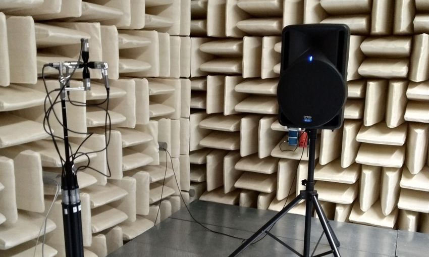
8th Berlin Beamforming Conference 2020                                               Ernst et al.

        Figure 1: Intel Realsense D435 depth- (top) and T265 pose- (bottom) camera

               Figure 2: Measurement setup of the cavity calibration procedure

   The speaker in the phase calibrator is driven with white noise between 50 Hz and 6 kHz.
Two measurements for two different MEMS microphones are conducted with a measurement
period of 60 seconds. The two transfer function between the reference sensor and the MEMS
microphones are estimated using the approach of Welch [12]. In figure 3 the resulting difference
in amplitude and phase of the transfer function between two MEMS microphones are shown.

                                               5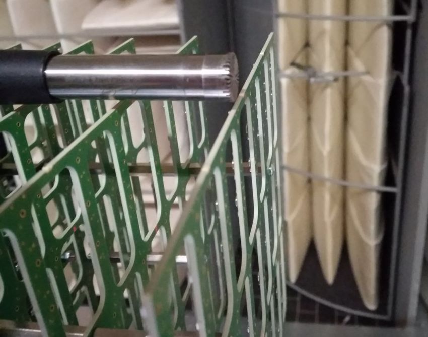
8th Berlin Beamforming Conference 2020                                             Ernst et al.

         Figure 3: Amplitude and phase difference between two MEMS microphones

The difference in amplitude between 60 Hz and 6 kHz is 0.25 dB at most whereas the difference
in phase is up to 4 degree at low frequencies below 100 Hz. Above 1 kHz, the measured phase
differences between two MEMS microphones is below ± 1 degree.

3.2 Farfield Calibration

A calibration in the free field was carried out in an anechoic room. During the measurements
a foam covered windtunnel was present in the anechoic room, which limits the free field
condition. Nevertheless a speaker was placed approximately 1.5 m above the non-reflective
ground. The reference microphone (G.R.A.S. 1/2” freefield) and the MEMS microphone array
were placed in 2 m distance to the speaker as close (≈ 12.7 mm) as possible to each other
(figure 6).
In figure 4 the difference in amplitude and phase between the reference microphone and a
MEMS microphone is shown. The amplitude is normalized at 1 kHz and is within ± 2 dB
from 50 Hz to 8 kHz and within ± 1 dB from 70 Hz up to 5 kHz. The difference in the phase is
within ± 60 degree from 50 Hz to 7 kHz.

3.3 Influence of MEMS-Array on the acoustic field

Due to the size of the PP512 MEMS array (≈ 0.2 x 0.2 x 0.2 m) which is much larger than the
wavelength at 6 kHz (≈ 0.06 m) the PCBs might have an influence on the acoustic field itsself.
Therefor a reference microphone was placed in the center of PP512 MEMS array (see figure 7)
and again a speaker is placed in 2 m distance in an anechoic room. The speaker is driven by
white noise. In the next measurement the PP512 MEMS array is removed and only the reference

                                              6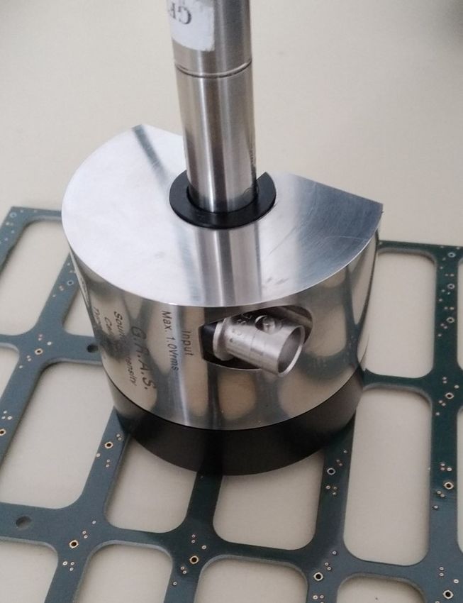
8th Berlin Beamforming Conference 2020                                               Ernst et al.

Figure 4: Amplitude and phase difference between a MEMS and a reference microphone
          (G.R.A.S. 1/2” freefield).

microphone is left. These two measurements are compared regarding the amplitude spectrum
of the reference microphone (see figure 5). Up to 3 kHz the difference in amplitude is less than
± 2 dB. Above 3 kHz the difference increases up to 8 dB and thus the influence of the presence
of the PP512 MEMS array cannot be neglected.

Figure 5: Difference in the amplitude spectrum of the reference microphone with and without
          the presence of the MEMS microphone (see figure 7).

                                               7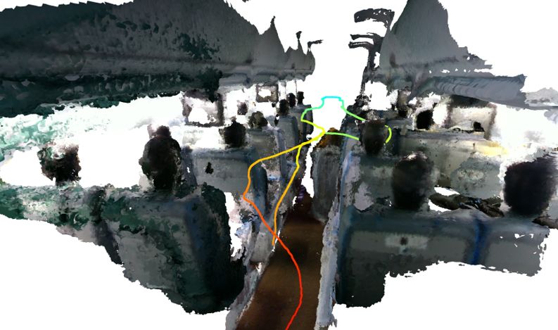
8th Berlin Beamforming Conference 2020                                                 Ernst et al.

 Figure 6: Measurement setup of the free field
           calibration procedure.             Figure 7: Measurement setup to measure the
                                                        influence of the PP512 MEMS ar-
                                                        ray on the acoustic field with a ref-
                                                        erence microphone.

3.4 Comparison to 3D-PP Probe

In this section the PP512 MEMS array is compared to a classical intensity probe from G.R.A.S.
of the type 50VI-1. Both probes were placed again 2 m in front of the loudspeaker in an anechoic
room. The speaker was driven by white noise and two different measurements were carried out.
In figure 10 the acoustic intensity normalized at 1 kHz is shown for both, the classical pp-probe
and the PP512 MEMS array. The acoustic intensity was calculated according to section 2.2
and position of the virtual intensity probe was chosen to the exact location of the pp-probe. No
phase or amplitude correction was performed. Between 200 Hz and 1.5 kHz the difference in
acoustic intensity is less than 1 dB. Below and above this frequency range the acoustic intensity
estimated by the PP512 MEMS array is up to 8 dB higher than the estimation of the pp-probe.

3.5 Aircraft Cabin - Dornier 728 ground demonstrator

The last measurement in this paper is carried out in an aircraft cabin demonstrator with inte-
grated shakers behind lining to simulate the acoustic environment inside a real aircraft ([5],[4]).
A time signal recorded during flight inside the cabin of an Airbus A320 was used to drive the
shaker. As described in section 2.3 the tracking system was used to record the position and
orientation of the PP512 MEMS array as well as an point cloud which is converted to a 3D-
Model. In figure 11 the 3D-Model and the camera position is shown for one measurement. The
quality of the 3D-Model could be improved a lot with the given information, but is not in the
field of interest of the authors. Nevertheless a 3D-Model and a position estimation of the hand-
held PP512 MEMS array is necessary to have a useful interpretation of the three dimensional
acoustic intensity quantities.

                                                8
8th Berlin Beamforming Conference 2020 Ernst et al.
Figure 8: Measurement setup to measure the Figure 9: Measurement setup to measure the
acoustic intensity with a PP-probe. acoustic intensity with the PP512
MEMS array.
Figure 10: Acoustic intensity normalized at 1 kHz for the measurement setup in figure 8 and 9
Again the acoustic intensity is calculated according to section 2.2 at 343 positions inside the
array for each timeblock of 42.66 ms and for each narrow band frequency. Each timeblock is
associated with the position an orientation given by the position tracking system at the center
time of the timeblock. Assuming a maximum velocity of array movement of 0.5 m/s the ac-
curacy of the acoustic intensity mapping is in the order of 1 cm and the acoustic frequency is
shifted due to the doppler effect by at most 0.15 %. The resulting data has a high spatial an
non-equidistant resolution. A voxel downsampling approach is performed to reduce the data
size as well as complexity and reduces the required averaging time of classical pp-probe mea-
surements. Voxel downsampling means that an equidistant grid of 60 mm resolution is created
and all the scattered position data is averaged at the nearest grid point. In figure 12 the resulting
acoustic intensity is shown for three different 3rd octave bands (1, 2 and 4 kHz) measured with
the PP512 MEMS array near the lining of the aircraft cabin at x = -0.4 m.
98th Berlin Beamforming Conference 2020 Ernst et al.
Figure 11: 3D-Model and path of the camera in the Dornier 728 ground demonstrator.
Figure 12: Acoustic intensity level at the 3rd octave bands 1, 2 and 4 kHz and a voxel down-
sampling of 60 mm.
108th Berlin Beamforming Conference 2020 Ernst et al.
4 CONCLUSION
The use of MEMS as acoustic intensity probe was shown for an arbitrary microphone layout
and implemented using a FPGA based data aquisition system. It was shown that the estimation
of the acoustic intensity can be seen as a kind of beamformer where the steering vectors are the
weighting factors of the Taylor expansion. A tracking system consisting of Intel Realsense cam-
eras was shown and found out to be very robust against fast movements and a position accuracy
below 1 mm at laboratory test in a limited field of movement of 30 cm. The calibrations proce-
dures for MEMS microphones are time consuming and requiring a precise handling regarding
positioning of the calibrator on the sound hole of the MEMS microphones. Nevertheless for
frequencies below 6 kHz a commercially available phase calibrater can be used to perform the
relative calibration of MEMS microphones to each other regarding phase and amplitude. An
absolute calibration of the amplitude and phase can be done by a measurement in the free field
and comparison with a reference microphone. The influence of the microphone array geometry
on the acoustic field is not negligible and above 3 kHz the change in amplitude can increase up
to 8 dB. But even without any frequency response calibration of the MEMS microphones the
acoustic intensity can be measured in high spatial resolution and in complex environments such
as an aircraft cabin without any preinstallations.
References
[1] L. del Val, A. Izquierdo, J. J. Villacorta, and L. Suárez. “Using a planar array of MEMS
microphones to obtain acoustic images of a fan matrix.” Journal of Sensors, 2017, 1–10,
2017. doi:10.1155/2017/3209142.
[2] F. Fahy. Sound Intensity. CRC Press, 1995. ISBN 0419198105. URL
https://www.ebook.de/de/product/6432207/frank_university_
of_southampton_fahy_sound_intensity.html.
[3] I. Hafizovic, C.-I. C. Nilsen, M. Kjølerbakken, and V. Jahr. “Design and implementation
of a MEMS microphone array system for real-time speech acquisition.” Applied Acoustics,
73(2), 132–143, 2012. doi:10.1016/j.apacoust.2011.07.009.
[4] C. S. Judith Kokavecz. “Microphone array technology for enhanced sound source locali-
sation in cabins.” AIA-DAGA 2013 Merano, 2013.
[5] C. S. Judith Kokavecz, Lasse Seemann. “Akustisch fliegen ohne abzuheben.” DAGA 2012.
[6] J. Kotus and G. Szwoch. “Calibration of acoustic vector sensor based on MEMS
microphones for DOA estimation.” Applied Acoustics, 141, 307–321, 2018. doi:
10.1016/j.apacoust.2018.07.025.
[7] J. S. Lawrence, K. L. Gee, T. B. Neilsen, and S. D. Sommerfeldt. “Higher-order estimation
of active and reactive acoustic intensity.” Acoustical Society of America, 2017. doi:
10.1121/2.0000610.
[8] C. Mydlarz, C. Shamoon, M. Baglione, and M. Pimpinella. “The design and calibration
of low cost urban acoustic sensing devices.” 2015.
118th Berlin Beamforming Conference 2020 Ernst et al.
[9] S. Orlando, A. Bale, and D. Johnson. “Design and preliminary testing of a MEMS micro-
phone phased array.” In Proceedings on CD of the 3rd Berlin Beamforming Conference,
24-25 February, 2010. 2010. ISBN 978-3-00-030027-1. URL http://bebec.eu/
Downloads/BeBeC2010/Papers/BeBeC-2010-21.pdf.
[10] B. Piper, T. Koukoulas, R. Barham, and R. Jackett. “Measuring mems microphone free
field performance using photon correlation spectroscopy.” 2015.
[11] R. P. Wagner and S. E. Fick. “Pressure reciprocity calibration of a MEMS microphone.”
The Journal of the Acoustical Society of America, 142(3), EL251–EL257, 2017. doi:
10.1121/1.5000326.
[12] P. Welch. “The use of fast Fourier transform for the estimation of power spectra: A
method based on time averaging over short, modified periodograms.” IEEE Transactions
on Audio and Electroacoustics, 15(2), 70–73, 1967. doi:10.1109/tau.1967.1161901. URL
http://dx.doi.org/10.1109/TAU.1967.1161901.
[13] R. White, J. Krause, R. D. Jong, G. Holup, J. Gallman, and M. Moeller. “MEMS mi-
crophone array on a chip for turbulent boundary layer measurements.” In 50th AIAA
Aerospace Sciences Meeting including the New Horizons Forum and Aerospace Exposi-
tion. American Institute of Aeronautics and Astronautics, 2012. doi:10.2514/6.2012-260.
[14] C. P. Wiederhold, K. L. Gee, J. D. Blotter, S. D. Sommerfeldt, and J. H. Giraud. “Com-
parison of multimicrophone probe design and processing methods in measuring acoustic
intensity.” The Journal of the Acoustical Society of America, 135(5), 2797–2807, 2014.
doi:10.1121/1.4871180.
[15] Q.-Y. Zhou, J. Park, and V. Koltun. “Open3D: A modern library for 3D data processing.”
arXiv:1801.09847, 2018.
12You can also read