Preliminary Walking Experiments with Underactuated 3D Bipedal Robot MARLO
←
→
Page content transcription
If your browser does not render page correctly, please read the page content below
2014 IEEE/RSJ International Conference on
Intelligent Robots and Systems (IROS 2014)
September 14-18, 2014, Chicago, IL, USA
Preliminary Walking Experiments with Underactuated 3D Bipedal
Robot MARLO
Brian G. Buss1 , Alireza Ramezani2 , Kaveh Akbari Hamed1 , Brent A. Griffin1 ,
Kevin S. Galloway3 , Jessy W. Grizzle1,2
Abstract— This paper reports on an underactuated 3D biped [13]. The robot PETMAN is fully actuated but re-
bipedal robot with passive feet that can start from a quiet alizes an underactuated gait that includes heel strike, foot
standing position, initiate a walking gait, and traverse the roll, and toe off, while responding impressively to lateral
length of the laboratory (approximately 10 m) at a speed
of roughly 1 m/s. The controller was developed using the shoves; its control system is based on capture-points
method of virtual constraints, a control design method first [10]. The bipedal robots M2V2 and COMAN are both
used on the planar point-feet robots Rabbit and MABEL. underactuated due to series elastic actuation, and both
For the preliminary experiments reported here, virtual have feet with ankles that are actuated in pitch and roll.
constraints were experimentally tuned to achieve robust M2V2 excels at push recovery using capturability-based
planar walking and then 3D walking. A key feature of the
controller leading to successful 3D walking is the particular control [15]. While COMAN uses ZMP style walking, it
choice of virtual constraints in the lateral plane, which is demonstrating improved energy efficiency and handles
implement a lateral balance control strategy similar to significant perturbations while standing. BIPER-3 was
SIMBICON. To our knowledge, MARLO is the most highly an early 3D biped which demonstrated dynamic balance;
underactuated bipedal robot to walk unassisted in 3D. its feet made only point contact with the ground, so the
I. INTRODUCTION
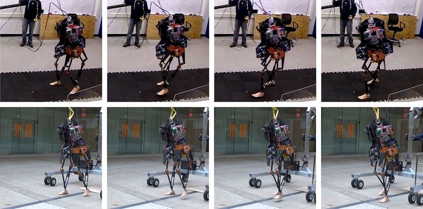
This paper presents experimental results on underac-
tuated 3D bipedal walking. The robot MARLO shown in
Fig. 1 has walked both indoors and outdoors on passive
prosthetic feet.
This research uses a 3D ATRIAS-series biped [1], [2]
to inspire the development of control laws that naturally
accommodate underactuation in bipedal locomotion. An
important reason for studying underactuation is that even
a fully actuated 3D robot can become underactuated
when walking. The source of underactuation may be
planned (as when seeking to execute a human-like
rolling foot motion) or unanticipated (such as when an
uneven walking surface precludes three non-collinear
points of contact, or even “worse”, when the object
under the foot rolls or causes slipping [3]). Traditional
ZMP-based walking control strategies explicitly try to
avoid such underactuation [4].
The vast majority of 3D bipedal robots use locomotion
algorithms that require full actuation [5]–[9]. Important
exceptions include PETMAN [10], M2V2 [11], CO-
MAN [12], Denise [13], Biper-3 [14], and the Cornell
1 Dept. of Electrical Engineering and Computer Science, 2 Dept.
of Mechanical Engineering, University of Michigan, Ann Arbor,
MI {bgbuss,aramez,kavehah,griffb,grizzle} Fig. 1: MARLO is an ATRIAS 2.1 robot designed by
@umich.edu
3 Dept. of Electrical and Computer Engineering, United States Naval
Jonathan Hurst and the Dynamic Robotics Laboratory at
Academy, Annapolis, MD kgallowa@usna.edu Oregon State University. (Photo: Joseph Xu)
978-1-4799-6934-0/14/$31.00 ©2014 IEEE 2529
Authorized licensed use limited to: Northeastern University. Downloaded on January 25,2021 at 22:34:07 UTC from IEEE Xplore. Restrictions apply.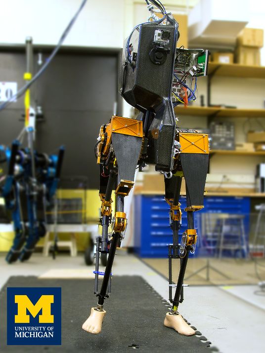
zT
machine was never statically stable. The Cornell biped                                                    yT
and Denise are quasi-passive robots that use specially                                                    xT
shaped feet to achieve lateral stability. It is hoped that
                                                                                           q2L                 q3R
the ATRIAS-series robots will prove to be significantly
more energy efficient than PETMAN, and capable of                                                    p0
more agile gaits than the other robots cited. This early-                                   q3L                               q1R
                                                                                                                     q2R             q2R
stage paper is far less ambitious, focusing on preliminary
                                                                                           qKA,L
control results for 3D walking.
   The feedback control law used here builds on previous
work by the authors and colleagues for underactuated                                  zW                                     zW                qKA,R
                                                                                                                     qKA,R
bipedal robots [16]. The method of virtual constraints                                     yW                                       yW
has been extended to the 3D setting in [2], [17]–[19] and                                  xW
others. Extensive experimental work had been performed                                             (a)                                   (b)
for underactuated planar gaits [16], [20]–[23], and refer-
ence [19] reported on the use of virtual constraints for an                  Fig. 2: Mechanical structure and coordinates for
experimentally-realized fully actuated (flat-footed) 3D                      MARLO. (a) Conceptual diagram of rigid body model.
walking gait. This paper reports for the first time on                       (b) Each leg is physically realized by a four-bar linkage.
underactuated walking in 3D using the method of virtual                      The knee angle qKA,R is related to the angles of the upper
constraints.                                                                 links as qKA,R = q2R − q1R .
   The remainder of the paper is organized as follows.
Section II provides a brief description of the robot
used in the experiments. Section III summarizes the                             Each leg consists of a four-bar linkage driven by
concept of virtual constraints as a control and gait design                  brushless DC (BLDC) motors connected to the upper
methodology; further details on these topics are available                   two links through 50:1 harmonic drives and series
in [2], [24]. Section IV presents experiments in 2D                          springs. The legs connect to the torso through coaxial
locomotion that are aimed at using leg retraction [25],                      pin joints. Two BLDC motors in the torso actuate the
[26] to augment the robustness of the gait to perturba-                      hips in the lateral plane.
tions. Section V describes a method for gait initiation                         In single support the robot model has 13 degrees of
in 3D; it allows the robot to stand quietly on passive                       freedom and 6 actuators. Figure 2 illustrates a choice
prosthetic feet and then take a first step without any                       of coordinates. The orientation of the torso with respect
external assistance. Section VI presents experiments on                      to an inertial world frame is represented by ZYX Euler
3D walking, where the gait is initiated from a standing                      angles qzT , qyT and qxT (yaw, roll, and pitch, respec-
position and achieves an average walking speed of 1                          tively). As shown in Fig. 2 (b), the relative angles of the
m/s. Conclusions are given in Sect. VII.                                     upper links of the right leg are denoted by q1R and q2R .
                                                                             Not shown in the figure are the coordinates at the output
            II. HARDWARE DESCRIPTION                                         shafts of the corresponding harmonic drives, denoted
                                                                             by qgr1R and qgr2R . The difference qgr1R − q1R is the
   MARLO is an ATRIAS-series robot designed and
                                                                             spring deflection. Coordinates for the left leg are defined
built at Oregon State University. The robot is 1 meter tall
                                                                             analogously. The coordinate vector q is defined as
at the hips and has a mass of 55 kg. The torso accounts
for approximately 40% of the total mass of the robot and
                                                                                q := (qzT , qyT , qxT , q1R , q2R , q1L , q2L ,
has room to house1 the onboard real-time computing,
LiPo batteries, and power electronics for the motors.                                           qgr1R , qgr2R , q3R , qgr1L , qgr2L , q3L )> , (1)
Most of the remaining mass is concentrated in the two                        in which the first seven components are unactuated and
hips, leaving the legs very light. For these experiments,                    the last six components are actuated. The input torques
the nominal point feet of the robot were replaced with                       at the actuated coordinates are defined as
commercial passive prosthetic feet. For the purposes of
control design, a point-foot model is assumed, with the                                u := (u1R , u2R , u3R , u1L , u2L , u3L )> .                    (2)
caveat that the feet do provide some anti-yaw torque;
                                                                               Encoders measure the angles of all internal joints.
see [2, Eqn. (5)].
                                                                             An IMU measures the orientation of the torso relative
  1 For the experiments reported here, the real-time computer and the        to the world frame. MARLO does not use a camera,
batteries were off board. The associated cables are visible in the videos.   and it presently lacks contact sensors at the leg ends to

                                                                         2530

Authorized licensed use limited to: Northeastern University. Downloaded on January 25,2021 at 22:34:07 UTC from IEEE Xplore. Restrictions apply.
detect impacts. Impacts are detected by measuring the where, for i ∈ {R, L}, qgrLA,i is equal to the angle
spring deflection in the series-elastic actuators driving between the torso and the line segment between the hip
the sagittal coordinates of the legs. A major upgrade in and the leg end and qgrKA,i is equal to the knee angle
sensing is planned. when the leg springs are not deflected. qHip,i is the angle
For a more detailed description of the hardware, see of hip i relative to the torso in the lateral plane. With
[2], [24]. this choice, the virtual constraints have vector relative
degree two [16].
III. CONTROL METHODOLOGY
The desired evolution of the controlled variables
Virtual constraints are holonomic output functions de- h0 (q) is chosen as
fined in the configuration space of a mechanical system
and zeroed through the action of a feedback control law. hd (θ) = B(s(θ), α) (7)
Virtual constraints are used to coordinate the links of the
where B(s, α) is a vector of Bézier polynomials in s
legged robot during a step, with the goal of inducing
with coefficients α = α0 · · · αM .
an asymptotically stable periodic walking gait. In its
preferred implementation, the constraints are determined B. Zeroing the outputs to impose the constraints
through model-based parameter optimization [2], [16], Inverse dynamics may be used to zero the outputs
[18], [19]. Here, because the model of MARLO is not (3) and thereby enforce the virtual constraints. Due
yet fully identified, they are designed by hand; see also to uncertainty in the position of the torso center of
[27] and [20]. A brief summary of the methodology mass, unmodeled dynamics in the harmonic drives, and
follows. a limited ability to determine ground contact, these pre-
A. Forming the constraints liminary experiments use a more classical feedforward
The most basic form of the virtual constraints is and PD control action
KD KP
y := h(q) := h0 (q) − hd (θ(q)), (3) u(q, q̇) = uFF (q, q̇) + T ẏ + 2 y . (8)
ε ε
where h0 (q) specifies the vector of variables to be The feed forward term uFF (q, q̇) primarily implements
controlled and hd (θ) is the desired evolution of the an approximate form of gravity compensation. The in-
controlled variables as a function of θ(q). The gait- vertible matrix
timing variable θ(q) replaces time in parameterizing the −1
motion of the robot. Consequently, θ(q) is selected to 1/2 1/2 0 0 0 0
be strictly monotonic (increasing or decreasing) along 0 0 0 1/2 1/2 0
nominal walking gaits. −1 1 0 0 0 0
T = (9)
As in Rabbit and MABEL, θ(q) is chosen as the 0 0 0 −1 1 0
absolute angle of the line connecting the stance leg end 0 0 1 0 0 0
to the hip in the sagittal plane, i.e., 0 0 0 0 0 1
relates the components of the output function y(q) to the
(
π
− qxT − q1R +q 2R
in right stance
θ(q) := π2 2
q1L +q2L (4) input variables u. The diagonal gain matrices KP and
2 − qxT − in left stance.
2
KD and the scalar ε were chosen such that the matrix
It is convenient to normalize θ(q) to the interval [0, 1] s2 I + KεD s + Kε2P is Hurwitz.
and call it s(q), as
IV. PLANAR WALKING AND LEG
θ(q) − θ+ RETRACTION
s(q) := , (5)
θ− − θ+
Initial testing was performed with the robot attached
where θ+ and θ− represent the values of θ at the to a boom which constrains the lateral motion of the
beginning and end of a typical walking step. torso. An encoder measuring the pitch angle of the torso
A nominal set of controlled variables is was used instead of the IMU-derived pitch angle for
some of the planar experiments. The purpose of these ex-
1
qgrLA,R 2 (qgr1R + qgr2R )
qgrLA,L 1 (qgr1L + qgr2L )
2 periments was to identify and correct hardware issues, to
form an idea of the quality of the model, and to develop
qgrKA,R qgr2R − qgr1R
h0 (q) = =
, (6)
a robust planar gait as a basis for 3D locomotion. The
qgrKA,L qgr2L − qgr1L
qHip,R q3R control design in this section uses the nominal controlled
qHip,L q3L variables (6), with the desired (lateral) hip angles set to
2531
Authorized licensed use limited to: Northeastern University. Downloaded on January 25,2021 at 22:34:07 UTC from IEEE Xplore. Restrictions apply.Leg angle (deg) 1.6
Step Speed (m/s)
200
1.4
1.2
180
nominal 1
enhanced 0.8
160
0 0.2 0.4 0.6 0.8 1 0.6
s 1.6
Step Speed (m/s)
Fig. 3: Desired swing leg angles with and without 1.4
enhanced swing leg retraction. 1.2
1
0.8
constants. The desired evolution of the virtual constraints
0.6
in the sagittal plane was initially designed as in [2] 0 20 40 60
on the basis of the CAD model of the robot, and Step Number
then subsequently adjusted by hand to improve foot
clearance; see the video [28]. The process of improving Fig. 4: Step speed during two experiments where the
the robustness of this gait led to leg retraction, which is boom was pushed. Both experiments used point feet. In
described next. each plot, the heavy red stems indicate steps where the
experimenter was in contact with the boom. Significant
A. Swing leg retraction left-right asymmetry due to the boom appears in the
Humans and animals often brake or reverse the swing period two oscillation in the step speed. (Top) Without
leg just before impact. This behavior, termed swing enhanced swing leg retraction, the velocity increased
leg retraction, has been shown to improve stability after the push and remained higher than normal for
robustness in spring-mass models of running [25]. multiple steps until the robot tripped and eventually fell.
We implement swing leg retraction by increasing the (Bottom) With enhanced swing leg retraction, the step
desired swing leg angle near the end of a step while velocity returns to nominal within one or two steps after
leaving the final desired swing leg angle unchanged. Fig- the push. In this experiment the robot rejected multiple
ure 3 compares the Bézier polynomials for the nominal pushes before falling.
and modified swing leg angle virtual constraints. The
modified evolution was selected by adjusting a single
Bézier coefficient and running a series of walking exper- A second set of experiments was conducted in a new
iments during which the boom was occasionally pushed. laboratory for 3D locomotion. In this set up, the boom
More exaggerated leg retraction tended to cause the was limited to a half circle. The desired knee angles
robot to “stomp” without noticeably improving stability were further modified to accommodate the prosthetic
robustness. feet without scuffing. We verified that the control design
remained stable and robust when the torso pitch encoder
B. Experimental results measurement was replaced with the lower bandwidth
Planar walking experiments confirmed that swing leg IMU-derived pitch angle, and when prosthetic feet were
retraction enhanced disturbance rejection when walking used instead of point feet. The robot successfully walked
with point feet. External disturbances were induced over slightly uneven terrain while subjected to external
by pushing on the boom as MARLO walked. The disturbances; a video is available online [28].
initial experiments were conducted on a circular boom,
V. 3D GAIT INITIATION
previously used for the robot MABEL [21]. Figure 4
shows the step speeds during two experiments (without Walking in 3D requires a method for transitioning
and with enhanced swing leg retraction) where the from a standing position to a periodic orbit correspond-
boom was pushed from behind while the robot walked. ing to a walking gait. Our strategy for gait initiation
With the nominal virtual constraint, the robot became consists of two parts, namely standing still, referred to
unstable and eventually fell after a single mild push. here as quiet standing, and a transition step from quiet
With enhanced swing leg retraction, the robot rejected standing to a sustained walking motion. The strategy
multiple pushes roughly increasing in intensity. used here was developed in [24].
2532
Authorized licensed use limited to: Northeastern University. Downloaded on January 25,2021 at 22:34:07 UTC from IEEE Xplore. Restrictions apply.A. Quiet standing per second, the joint commands switch from constant
Imagine the robot standing on flat ground, in a fixed set points to the virtual constraints. The robot rolls onto
posture, with the torso upright and the legs parallel the right leg and steps forward with the left leg (see
to the torso. Suppose further that the knees are bent curves in [24] and video at [28]). At leg impact, control
approximately 20◦ and the feet are flat on the ground. is passed to the steady-state walking controller described
In this posture, the width of the stance is approximately next.
30 cm, and the approximate left-right symmetry of the VI. 3D WALKING
robot ensures that the lateral component of the CoM is We now describe key modifications to the planar
between the feet, providing lateral static stability. Static walking controller which led to successful 3D walking.
stability in the sagittal plane is based on the following The essential change is in the choice of virtual con-
observation. Due to the feet being rigidly attached to straints defining the lateral hip control.
the shin (i.e., lower front link of the 4-bar linkage), It was known that the controlled variables defined in
increasing the knee bend “raises” the heel, that is, it (6) give rise to a periodic gait which is unstable [2], [18].
moves the CoP of the feet forward; on the other hand, To stabilize the lateral motion we designed alternative
straightening the knee “raises” the toe, that is, it moves virtual constraints inspired by the SIMBICON balance
the CoP backward. control strategy [29]. We first summarize the original
It follows that as long as the nominal knee angle is SIMBICON algorithm, then describe the modified ver-
not near the locking point, knee angle adjustment can be sion used in our experiments.
used to achieve a statically stable posture. This “passive”
method of quiet standing was used in the experiments A. Nominal SIMBICON algorithm
reported in Sect. VI. It is noted that active feedback SIMBICON is a framework for the control of bipedal
stabilization of quiet standing was used in [24]. walking or running. Variations of the algorithm have
To exit quiet standing, it is enough to straighten the been used in simulation of a variety of legged creatures
knees. The robot then pitches forward, rotating about [30], [31] and in experiments with a quadrupedal robot
the toes in the sagittal plane. The transition step can be [32]. It is based on a finite-state machine having a
triggered on the basis of pitch angular velocity. fixed target pose for each state. Within each state, PD
control is used to drive individual joints toward the
B. Transition step
corresponding target angles. The swing hip and the torso
A nominal standing posture is assumed, with the angle are controlled relative to the world frame. The
robot’s CoM initially moving forward at 0.17 m/s stance hip torque τA is computed from the torso torque
(roughly equivalent to the rotating about its toe at 10 τtorso and the swing hip torque τB as τA = −τtorso −τB .
degrees per second). The mechanical phase variable One additional element is needed to provide feedback
(5) is used to parameterize a set of virtual constraints for balance. The desired swing hip angle is updated
(3), with the controlled variables h0 (q) given by (6). continuously by a feedback law of the form
The desired evolution hd (θ) of the virtual constraints
is chosen to join “as closely as possible” the standing ψsw,d = ψsw,d0 + cp d + cd d˙ (10)
posture at s = 0 to the final posture at s = 1 of a where ψsw,d is the instantaneous target swing hip angle,
periodic walking gait having an average walking speed ψsw,d0 is the nominal target swing hip angle specified
of 0.75 m/s. In [24], this was posed as an optimization by the state machine, and d is the horizontal distance
problem for choosing the coefficients in a set of Bézier between the CoM and the stance ankle. The midpoint
polynomials in hd (θ). Starting from the nominal poly- between the hips is used as an approximation of the
nomials reported in [24], we found it straightforward to CoM. In 3D, the nominal algorithm uses the same
adjust the final swing foot position on the first step in balance strategy in both the frontal and sagittal planes.
order to accelerate the robot into a forward walk.
B. Virtual constraints for the swing hip
C. Sequencing The experiments reported in this paper use a modified
The transition step is initiated by the operator sending form of SIMBICON to compute the desired swing hip
a ramp command to rapidly straighten the knees by angle in the lateral plane. We do not use SIMBICON in
a fixed amount, which pitches the robot forward. The the sagittal plane. We define absolute hip angles
commanded change in left knee angle is greater than the
ψR = −qyT − q3R (11)
right so as to initiate a roll onto the right leg. When the
IMU registers the torso pitching forward at 10 degrees ψL = qyT − q3L (12)
2533
Authorized licensed use limited to: Northeastern University. Downloaded on January 25,2021 at 22:34:07 UTC from IEEE Xplore. Restrictions apply.so that both increase as the foot moves outward. We set C. Virtual constraints for the torso
ψst = ψR and ψsw = ψL in right stance; in left stance Our method for controlling the torso also differs
these definitions are reversed. slightly from the SIMBICON strategy. Absolute torso
Instead of adjusting the desired swing hip angle based angle control is easily accomplished by substituting
on the distance d as in (10), we use the absolute stance a virtual constraint on the torso roll in place of the
hip angle ψst . This angle can be thought of as a linear constraint on the stance hip. However, this may lead to
approximation of d. The desired angle is large stance hip angles. We make the tradeoff between
ψsw,d = ψsw,d0 + cp ψst , (13) torso and (relative) hip control explicit by defining a new
controlled coordinate
where ψsw,d0 and cp are control parameters.
This strategy causes the swing leg to approximately h0,st (q) = aγqyT + (1 − γ)(q3,st − bst ), (15)
mirror the stance leg in the lateral plane. One conse- where bst is the desired stance hip angle, and γ ∈ R.
quence of this strategy is that the swing foot generally Note that γ = 0 corresponds to relative hip angle control
moves inward during the beginning part of each step, (the nominal output), while γ = 1 corresponds to pure
and outward near the end. This is undesirable, as it torso control (as in SIMBICON). The quantity h0,st (q)
brings the feet closer together during the middle of the replaces q3R (in right stance) or q3L (in left stance) in
step, increasing the likelihood that the feet will collide. (6); the corresponding element of hd (θ) is set to zero.
It also increases tracking errors, particularly near the end The swing hip feedback torque is treated as a known
of the step where they result in poor foot placement. We disturbance on the torso. Its effect is canceled though
wish to modify (13) to reduce this inward motion. disturbance feedforward, which can be implemented by
It is also helpful to ensure that errors near the begin- changing a single element of the matrix T in (9). The
ning of each step are relatively small. Doing so reduces same result is achieved in SIMBICON by the choice of
unwanted yawing caused by large corrective torques τstance .
before the new “swing” foot is off the ground.
We do not modify the controlled coordinates (6) to
We address both of these issues simultaneously. To implement torso control in the sagittal plane as in the
reduce the inward motion of the swing foot we add lateral. However, adjusting the desired leg angles has
a term to the right hand side of (13) which depends the effect of biasing the torso forward or backward. In
on the gait phase variable s. We also add a correction several experiments the sagittal torso offset was updated
term which zeroes the error at s = 0 and vanishes as s in a step-to-step manner to regulate the walking speed.
approaches one. The resulting expression for the desired
swing hip angle is given by D. Experimental results
ψsw,d = (1 − s)3 ψsw − 3(1 − s)2 s (bsw + aqyT ) The goal of these preliminary 3D experiments was to
obtain a baseline walking controller, and to let the robot
+ 3(1 − s)s2 + s3 (ψsw,d0 + cp ψst ) (14)
walk as far as possible. Without the modified virtual
where a = −1 in right stance and a = 1 in left stance. constraints, the robot could take only six or seven steps.
The parameter bsw biases the value of ψsw,d in the Improved lateral stability resulting from the new virtual
middle of a step in order to keep the feet apart. When constraints resulted in numerous experiments in which
s = 0 this equation gives ψsw,d = ψsw , and when MARLO walked to the end of the laboratory, a distance
s = 1 it reduces to (13). Note that (14) defines ψsw,d as of roughly 10 meters. Several walking experiments were
cubic Bézier polynomial in s. It differs from the desired also performed outdoors, where MARLO was chal-
evolutions introduced in Section III as the coefficients lenged with mild slopes and ground variation. Snapshots
of the polynomial in (14) are updated continuously. To from videos of both indoor and outdoor walking are
write the virtual constraint 0 = ψsw,d − ψsw in the form shown in Fig. 6.
(3) we define Model uncertainty (particularly uncertainty in the
mass distribution of the torso) necessitated experimental
h0,sw (q) = 1 − (1 − s)3 q3,sw − 3(1 − s)2 sbsw tuning of the control parameters cp , bsw , γ, and of
+ 3s2 − 2s3 (a(1 + cp )qyT + ψsw,d0 − cp q3,st ) .
various torso offsets. We found that controlling torso
roll improves lateral swing foot placement. However,
This quantity replaces q3L (in right stance) or q3R (in with pure torso control (γ = 1), the hip angles were
left stance) in (6); the corresponding element of hd (θ) excessively large; setting γ = 0.7 led to a better
is set to zero. compromise. The robot successfully walked with cp
2534
Authorized licensed use limited to: Northeastern University. Downloaded on January 25,2021 at 22:34:07 UTC from IEEE Xplore. Restrictions apply.10 search Fellowship under Grant No. DGE 1256260.
Angle (deg) A A. Ramezani, B. A. Griffin, and J. W. Grizzle were
5
Torso Roll
B supported by NSF grants ECCS-1343720 and ECCS-
0 1231171. K. Akbari Hamed and K. S. Galloway were
−5 supported by DARPA Contract X0130A-B. Dennis
Schweiger and Dennis Grimard contributed greatly to
−10 the design of the robotics laboratory used in this work.
15 Jill Petkash, University of Michigan Orthotics and Pros-
Hip Angle (deg)
Absolute Stance
thetics Center, and Todd Salley, College Park, assisted
10
with the Tribute prosthetic feet used on the robot. Xingye
5 (Dennis) Da assisted with the outdoor experiments. J.
Grizzle thanks Russell Tedrake of MIT for hosting his
0
sabbatical in early 2013, which gave rise to some of the
−5 ideas in this paper.
0 5 10 15 20
Step Number R EFERENCES
Fig. 5: Beginning-of-step torso and hip angles during [1] J. Grimes and J. Hurst, “The design of ATRIAS 1.0 a unique
two 3D walking experiments. In (A), a fixed torso offset monopod, hopping robot,” Climbing and walking Robots and
was used. Adjusting the torso angle to control walking the Support Technologies for Mobile Machines, International
Conference on, 2012.
speed improved stability. [2] A. Ramezani, J. W. Hurst, K. Akbari Hamed, and J. W. Grizzle,
“Performance Analysis and Feedback Control of ATRIAS,
A Three-Dimensional Bipedal Robot,” Journal of Dynamic
Systems, Measurement, and Control, vol. 136, no. 2, Dec. 2013.
between 0.5 and 1.1, though the higher gains tended [3] IHMC Robotics Lab, “Atlas walking over randomness,” Online:
to cause more leg splay. http://www.youtube.com/watch?v=d4qqM7 E11s, Nov 2013.
Figure 5 illustrates the difference in torso and hip [4] A. Goswami, “Postural stability of biped robots and the foot-
angles resulting from different parameter choices. In the rotation indicator (FRI) point,” International Journal of Robotics
Research, vol. 18, no. 6, pp. 523–33, Jun. 1999.
experiment labeled (A), the SIMBICON gain cp was set [5] K. Hirai, M. Hirose, Y. Haikawa, and T. Takenake, “The de-
to 1.1 and the mid-stride swing hip bias bsw was -8 velopment of Honda humanoid robot,” in Proc. of the IEEE
degrees. In the experiment labeled (B), cp was set to International Conference on Robotics and Automation, Leuven,
Belgium, May 1998, pp. 1321–1326.
0.5 and bsw was -4 degrees during the transient steps [6] J.-Y. Kim, I.-W. Park, and J.-H. Oh, “Experimental realization
following gait initiation and was then set to -3 degrees. of dynamic walking of the biped humanoid robot KHR-2
Additionally, in (B) the torso offset was adjusted step- using zero moment point feedback and inertial measurement,”
Advanced Robotics, vol. 20, no. 6, pp. 707–736, Jan. 2006.
to-step to control walking speed. [7] H. Yokoi, Kazuhito and Kanehiro, Fumio and Kaneko, Kenji
and Fujiwara, Kiyoshi and Kajita, Shuji and Hirukawa,
VII. CONCLUSIONS “Experimental Study of Biped Locomotion of Humanoid Robot
An experimentally-tuned control law based on vir- HRP-1S,” in Experimental Robotics VIII, ser. Springer Tracts
in Advanced Robotics, B. Siciliano and P. Dario, Eds. Berlin,
tual constraints was demonstrated to induce unassisted Heidelberg: Springer Berlin Heidelberg, Jun. 2003, vol. 5, ch.
walking in a 3D bipedal robot having 13 degrees of Experiment, pp. 75–84.
freedom in single support and 6 actuators. Robustness [8] T. Takenaka, “The control system for the Honda humanoid
robot.” Age and ageing, vol. 35 Suppl 2, pp. ii24–ii26, 2006.
in the sagittal plane was enhanced through swing leg [9] H.-o. Lim and A. Takanishi, “Biped walking robots created at
retraction. Lateral control using virtual constraints based Waseda University: WL and WABIAN family.” Philosophical
on SIMBICON allowed the planar gait to be extended transactions. Series A, Mathematical, physical, and engineering
sciences, vol. 365, pp. 49–64, 2007.
to 3D walking. [10] G. Nelson, A. Saunders, N. Neville, B. Swilling, J. Bondaryk,
Planned improvements in sensing (including force- D. Billings, C. Lee, R. Playter, and M. Raibert, “PETMAN: A
torque sensors in the ankles and motion capture) will humanoid robot for testing chemical protective clothing,” Journal
facilitate identification of the torso mass distribution, of the Robotics Society of Japan, vol. 30, no. 4, pp. 372–377,
2012.
allowing for model-based control design. The robot will [11] J. Pratt and B. Krupp, “Design of a bipedal walking robot,” pp.
be challenged with difficult outdoor environments. 69 621F–69 621F–13, 2008.
[12] F. Moro, N. Tsagarakis, and D. Caldwell, “A human-like walking
ACKNOWLEDGMENT for the COmpliant huMANoid COMAN based on CoM trajec-
tory reconstruction from kinematic motion primitives,” in Hu-
This material is based upon work supported by manoid Robots (Humanoids), 2011 11th IEEE-RAS International
the National Science Foundation Graduate Student Re- Conference on, 2011, pp. 364–370.
2535
Authorized licensed use limited to: Northeastern University. Downloaded on January 25,2021 at 22:34:07 UTC from IEEE Xplore. Restrictions apply.Fig. 6: Video snapshots from two 3D walking experiments. Frames are 200 ms apart. Videos of indoor (top row)
and outdoor (bottom row) experiments are available online [28].
[13] S. H. Collins, A. Ruina, R. Tedrake, and M. Wisse, “Efficient controller with active force control for running on MABEL,” in
bipedal robots based on passive-dynamic walkers,” Science, vol. Int. Conf. on Robotics and Automation (ICRA), May 2012.
307, pp. 1082–85, 2005. [23] H.-W. Park, K. Sreenath, A. Ramezani, and J. Grizzle, “Switch-
[14] H. Miura and I. Shimoyama, “Dynamic walk of a biped,” ing control design for accommodating large step-down distur-
International Journal of Robotics Research, vol. 3, no. 2, pp. bances in bipedal robot walking,” in Int. Conf. on Robotics and
60–74, 1984. Automation (ICRA), May 2012.
[15] J. Pratt, T. Koolen, T. de Boer, J. Rebula, S. Cotton, J. Carff, [24] A. Ramezani, “Feedback control design for MARLO, a 3D-
M. Johnson, and P. Neuhaus, “Capturability-based analysis and bipedal robot,” PhD Thesis, University of Michigan, 2013.
control of legged locomotion, Part 2: Application to M2V2, a [25] A. Seyfarth, H. Geyer, and H. Herr, “Swing leg retraction: A sim-
lower-body humanoid,” The International Journal of Robotics ple control model for stable running,” Journal of Experimental
Research, vol. 31, no. 10, pp. 1117–1133, Aug. 2012. Biology, vol. 206, pp. 2547–2555, 2003.
[16] E. R. Westervelt, J. W. Grizzle, C. Chevallereau, J. Choi, [26] D. G. E. Hobbelen and M. Wisse, “Swing-leg retraction for limit
and B. Morris, Feedback Control of Dynamic Bipedal Robot cycle walkers improves disturbance rejection,” Robotics, IEEE
Locomotion, ser. Control and Automation. Boca Raton, FL: Transactions on, vol. 24, no. 2, pp. 377–389, 2008.
CRC Press, June 2007. [27] J. Grizzle, J. Hurst, B. Morris, H. Park, and K. Sreenath,
[17] A. D. Ames and R. D. Gregg, “Stably extending two-dimensional “MABEL, a new robotic bipedal walker and runner,” in American
bipedal walking to three,” in American Control Conference, New Control Conference, St. Louis, Missouri, June 2009.
York, U.S.A., Jul. 2007, pp. 2848–2854. [28] B. G. Buss, A. Ramezani, K. Akbari Hamed, B. A. Griffin,
[18] C. Chevallereau, J. Grizzle, and C. Shih, “Asymptotically stable K. S. Galloway, and J. W. Grizzle. Preliminary walking experi-
walking of a five-link underactuated 3D bipedal robot,” IEEE ments with MARLO. Youtube Playlist: http://www.youtube.com/
Transactions on Robotics, vol. 25, no. 1, pp. 37–50, February playlist?list=PLFe0SMV3hBCBQ-ZnDmCwczGECMUtI0WAg.
2009. [29] K. Yin, K. Loken, and M. van de Panne, “SIMBICON: Simple
[19] A. D. Ames, E. A. Cousineau, and M. J. Powell, “Dynamically biped locomotion control,” ACM Transactions on Graphics,
stable robotic walking with NAO via human-inspired hybrid vol. 26, no. 3, 2007.
zero dynamics,” in Hybrid Systems, Computation and Control [30] S. Coros, A. Karpathy, B. Jones, L. Reveret, and M. van de
(HSCC), Philadelphia, April 2012. Panne, “Locomotion skills for simulated quadrupeds,” ACM
[20] J. W. Grizzle, G. Abba, and F. Plestan, “Asymptotically stable Transactions on Graphics, vol. 30, no. 4, pp. 59:1–59:12, 2011.
walking for biped robots: Analysis via systems with impulse [31] T. Geijtenbeek, M. van de Panne, and A. F. van der Stappen,
effects,” IEEE Transactions on Automatic Control, vol. 46, no. 1, “Flexible muscle-based locomotion for bipedal creatures,” ACM
pp. 51–64, Jan. 2001. Transactions on Graphics, vol. 32, no. 6, 2013.
[21] K. Sreenath, H. Park, I. Poulakakis, and J. Grizzle, “A compliant [32] C. Gehring, S. Coros, M. Hutter, M. Bloesch, M. Hoepflinger,
hybrid zero dynamics controller for stable, efficient and fast and R. Siegwart, “Control of dynamic gaits for a quadrupedal
bipedal walking on MABEL,” International Journal of Robotics robot,” in Robotics and Automation (ICRA), 2013 IEEE Interna-
Research, vol. 30(9), pp. 1170–1193, 2011. tional Conference on, 2013, pp. 3287–3292.
[22] K. Sreenath, H.-W. Park, and J. Grizzle, “Design and exper-
imental implementation of a compliant hybrid zero dynamics
2536
Authorized licensed use limited to: Northeastern University. Downloaded on January 25,2021 at 22:34:07 UTC from IEEE Xplore. Restrictions apply.You can also read