CO2 profiling by space-borne Raman lidar
←
→
Page content transcription
If your browser does not render page correctly, please read the page content below
CO2 profiling by space-borne Raman lidar                                 ISTP 2019,
                                                                                          Toulouse,
            Paolo Di Girolamo1, Volker Wulfmeyer2, Andreas Behrendt2,                   20-24 May 19
                         Carmine Serio1, Davide Dionisi3
                 1Scuola   di Ingegneria, Università della Basilicata, Potenza, Italia
        2Institut fuer Physik und Meteorologie, Universitaet Hohenheim, Stuttgart, Germany
                                     3ISMAR-CNR, Roma, Italy

                                                          Motivation
                              • CO2 mixing ratio in the atmosphere has substantially
                                increased from values around 300 ppm in the fifties of
                                previous century to a current value of 415-420 ppm, with an
                                annual increasing rate of approximately 2 ppm.
                              • Approximately 50 % of CO2 amount produced through
                                fossil fuel combustion and other human activities is injected
                                in the atmosphere and accumulates in it, while the remaining
                                50 % is absorbed by the oceans and the terrestrial biosphere.
                              • Forests cover ~30% of the Earth’s global land area and store
                                large amounts of carbon captured from the atmosphere.
• In order to properly quantify this sink mechanism and its contribution to the carbon
  cycle, accurate measurements of the CO2 gradients between the forest floor and the top
  of the canopy, and their temporal variations, are urgently needed.

• This ultimately translates into the capability to perform accurate and high vertical and
  horizontal resolution measurements of CO2 mixing ratio profiles.
Although the space and ground network for CO2 monitoring has regularly expanded over the
past 50 years, it does not guarantee the necessary spatial and temporal resolution needed for
a quantitative analysis of sources and sinks.

Space sensors provide CO2 measurements above forest canopies, which do not allow to
properly estimate Gross Primary Production (GPP).

These observational gaps could be addressed with an active remote sensing system in space
based on the roto-vibrational Raman lidar technique.

                                                          ISTP 2019, Toulouse, 20-24 May 2019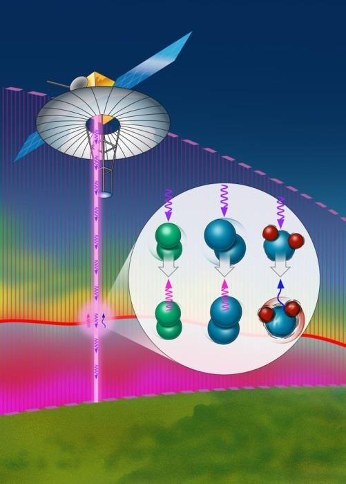
Raman lidar technique for CO2 profiling
Despite its important potential scientific impact, the CO2 vibrational Raman lidar technique has
received limited attention in the last 25 years both at theoretical and experimental level, mainly
because of the limited precision that this technique could guarantee, due to the limited cross-
sections and to the low concentration of the sounded species.

However, in the last decade, considerable technological progress has been achieved in the
design and development of solid-state laser sources with high optical power, large-aperture
telescopes and high-gain and quantum efficiency detectors.

This technological progress allows today reaching a new level of performance in the Raman
lidar measurements of CO2.

In a Raman system, CO2 profile measurements are possible, together with simultaneous
measurements of the temperature and water vapour mixing ratio profile and a variety of
additional variables (aerosol backscatter and extinction profiles, PBL depth, cloud top and base
heights, cloud optical depth).

                                                               ISTP 2019, Toulouse, 20-24 May 2019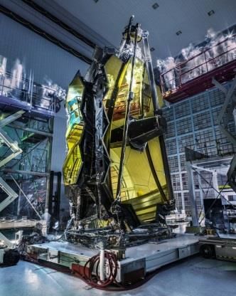
Observational requirements for CO2 profiling
In order to properly design and size a Space Raman lidar, observational requirements have to
be assessed and defined.
                                 Vertical variability in CO2
Seasonal and annual mean of CO2 vertical profiles reflect the combined influences of
surface fluxes and atmospheric mixing.
During the summer in the Northern Hemisphere, atmospheric CO2 concentrations are
generally lower near the surface than in the free troposphere, reflecting the greater impact of
terrestrial photosynthesis over industrial emissions at this time (Stephens et al., 2007).
Conversely, during the winter, respiration and fossil-fuel sources lead to high low-altitude
atmospheric CO2 concentrations at northern locations. The gradients are comparable in
magnitude in the two seasons, this being of the order of 10 ppm.

CO2 gradients between the forest floor and the top of the canopy are in the range 75-100
ppm in daytime and 10-50 ppm at night. Both ranges represented spring conditions when
canopy leaf area development is not completed.

The Space Raman lidar has to be designed                  • Vertical resolution: 200 m
and sized with the goal of allowing                       • Horizontal resolution : 50 km
measurements of these gradients.                          • Accuracy: 2-5 ppm

                                                            ISTP 2019, Toulouse, 20-24 May 2019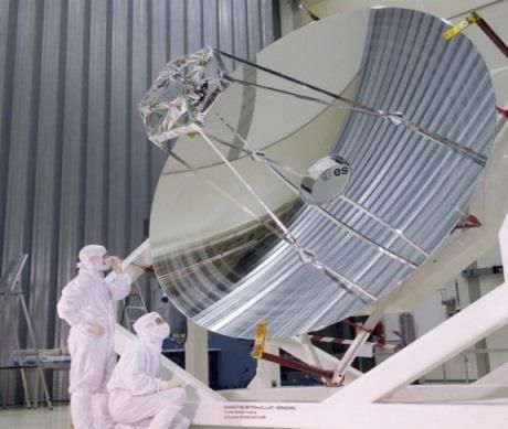
Mission Characteristics
The lidar setup considered in the present research effort heavily relies on the mission concept of
ATLAS proposed to the European Space Agency in response to the Call for Explorer-10
Mission Ideas. Simulations consider a sun-synchronous low Earth orbit, with an orbiting height
and speed of 450 km and 7 km/s, respectively. A dawn-dusk orbit with overpasses at 6/18 h
local time has been selected for the simulations.
Instrumental concept benefits from recent advances in solid-state laser, large-
aperture telescope, and detector technologies.
• frequency-tripled diode-laser pumped Nd:YAG laser
Transmitter • average power of 250 W at 355 nm
• new generation of pump chambers and diode lasers (demon. under dev. at UHOH)
• electrical-to-optical efficiency > 5 % (by improving power supply and diode
Slab amplifiers laser efficiencies, reducing electrical losses, optimizing pump chambers and
with single the laser conversion efficiency).
pulse energies of
12 J (5 times
• Inclusion of several amplification stages (3-4), each one embedding high-
higher) were density stacks of pumping diodes
demonstrated in • Use of diode laser pumping determines radiative cooling to be sufficient.
Liu et al. (2017).
A pulse energy • Far less complex Does frequency stabilization unit,
>100 J in Mason than, e.g., for ADM not beam shaping optics,
et al. (2017) . or EarthCARE. require: specific operational modes (repet. rates and bursts).
ISTP 2019, Toulouse, 20-24 May 2019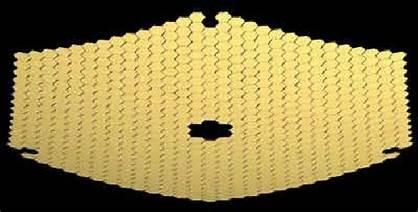
Mission Characteristics
• large-aperture, lightweight telescope, 4 m diameter
Receiver
• Different technological solution:
rigid primary mirror (single physical element or segmented
optics),
Rigid central mirror with folded deployable outer sections
inflatable optics
• several glass materials (e.g. Zerodur, SiC, etc.) with
appropriate low weight and thermal stability properties for
this type of space application
• no astronomical quality needed (no diffraction-limited
performances (swe
• In the present mission concept, the Raman lidar collects five primary
lidar signals:
CO2 vibrational Raman signal PCO2 z
water vapour roto-vibrational Raman signal PH O z
2
O2-N2 high- and low-quantum number
rotational Raman signals PloJ(z) & PHiJ(z)
elastic backscatter signal @ l0 Pl z
0
7 km s-1
7.5 m Horizontal and vertical signal averaging
7.5 m to reduce signal statistical uncertainties.
7.5 m Vertical resolution Dz=200 m
Horizontal resolution Dh=50 km
0.01 s
70 m
obtained with an time integration of 7.14 s
ISTP 2019, Toulouse, 20-24 May 2019
An Input CO2 mixing ratio profile data for the Simulator
was generated which accounts for different vertical 10000
gradients associated with the conflicting contributions of
terrestrial photosynthesis and industrial emissions, and
CO2 capturing within forest canopy. This input profile
includes a : 1000
• 10 ppm increase at an altitude of 2 km from a value of
400 ppm to one of 410 ppm, introduced in order to
Height (m)
simulate the daytime CO2 depletion taking place within 100
the mixed layer. In addition to this;
• 50 ppm decrease is considered at an altitude of 50 m
above the surface level, which is intended to represent
CO2 capturing within forest canopy. 10
• Other atmospheric quantities considered in the
simulation include:
vertical profiles of pressure, temperature, and 1
humidity from the U.S. Standard Atmosphere 1976 300 320 340 360 380 400 420 440 460 480 500
xCO2
atmospheric reference model;
Aerosol optical properties from the median aerosol
extinction data from the ESA ARMA Model.
The Space Raman lidar has to be designed
• Vertical resolution: 200 m
and sized with the goal of perfomimg
• Horizontal resolution : 50 km
measurements allowing to resolve these
• Accuracy: 2-5 ppm
gradients.
Simulation results
                                                                       5000
                                                                                         night time
An assessment of the expected system performance has                                     ZA=65°
been performed based on the application of an
                                                                       4000
analytical simulation model developed at University of
Basilicata.
                                                                       3000
Considering a vertical and horizontal resolution of 200

                                                          Height (m)
m and 50 km, respectively, the statistical uncertainty
(precision) affecting CO2 mixing ratio profile                         2000
measurements is not exceeding 5 ppm at night and 60
ppm in daytime from the surface up to an altitude of 5
km.                                                                    1000

Night-time performance is acceptable, but daytime is NOT.
                                                                          0
                                                                              1    10                 100
                                                                                  DxCO2/xCO2
However, so far we have been exploiting only the Raman                            Dx (ppm)
signal in the anti-Stokes 2v2 vibrational band.
CO2 Spectroscopy
Fermi resonance results in the splitting of two vibrational bands that have nearly the same
energy and symmetry in both IR and Raman spectroscopies. The two bands are usually a
fundamental vibration and either an overtone or combination band.
As a result, two strong bands are observed in the spectrum, instead of the expected strong and
weak bands. It is not possible to determine the contribution from each vibration because of
the resulting mixed wave function.
The three fundamental vibrations of CO2 are v1= 1337 cm-1, v2=667 cm-1, v3=2349 cm-1.
As a result of Fermi resonance, two strong bands are present, with frequencies v1=1337 cm-1
and 2v2(2 x 667 cm-1)=1334 cm-1.

              Stokes branch                                                                           Anti-Stokes branch
                                                               105
                                                                                                   Q-branch
                                                               104         Cabannes line           Total intensity of rotational Raman wings
                                                               103
                                                                                 pure-rotational Raman spectrum
                                          Relative intensity

                                                               102
                                                                                                 Vibrational Raman spectra
                                                               101

                                                               100
                                                                                                       O2
                                                                                                                       N2                      H2O (n1)
                                                               10-1

                                                               10-2
                                                                                           CO2 (n1)
                                                                    -3
                                                               10                   CO2 (2n2)
                                                                    -4
                                                               10
                                                                     520 530
                                                                          0 540 550 560 570 580 590 600 610 620 630 640 650 660 670
                                                                                             1556           2331                                 3562
                                                                           2v2=1334  cm-1        Wavelength , nm
           v1=-1337 cm-1 2v =-1334 cm-1                                                          Wave number (cm-1)
                                                                                    v =1337 cm-1
Thus, measuring the Raman lidar echoes from the two bands v1 and 2v2 both in the Stokes
and anti-Stokes branches, the intensity of the CO2 Raman lidar signal can be increased by a
factor of 4 to 5.
5000
This solution can be implemented in night time
ZA=65°
combination with a reduction of the receiving
field-of-view from 25 mrad to 10 mrad. 4000
This traslates into a statistical uncertainty
(precision) affecting CO2 mixing ratio profile 3000
Height (m)
measurements not exceeding 0.5 ppm at night
and 5 ppm in daytime from the surface up to an
2000
altitude of 5 km.
1000
0
1 10 100
0.1 1
DxCO2/xCO2 10
Dx (ppm)Measured parameters/expected performances
Clear-sky conditions
Accuracy estimated with experimentally-validated performance model (Di Girolamo et 15000
15000
al. 2006, 2018)
Resolution FOV=25 mrad
FOV=25 mrad
Variable (vertical/horizontal Precision Night time
Night time
) 12000 Daytime 12000 Daytime
Water vapor mixing ratio 200 m / 50 km 2-20 %
Temperature 200 m / 50 km 0.4-0.75 K 9000 9000
Relative humidity 200 m / 50 km 2-20 %
Height (m)
Height (m)
Planetary boundary layer height 100 m / 5 km 100 m 6000 H2O 6000 T
50-100 m / 10-50 1-3 % &
Particle backscatter & extinction
km 3-20 %
3000 3000
Cloud distribution 50-100 m / 5 km 50-100 m
Cloud optical depth 50 km 5%
0 0
0 5 10 15 20 0,2 0,3 0,4 0,5
Dq/q (%) DT (K)
• No ancillary data needed
500 profiles/hour, i.e.,
~12,000 profiles/day • Errors provided with each retrieved profile
(opposed to ~1200 • Clear air, above clouds, through broken
radiosoundings); clouds & through/below overcast thin
clouds
1st International Conference on Space Lidar Technology - (ICOSLA 2018), Beijing (China), 25-27 November 2018Summary • An accurate quantitative assessment of the various components of the carbon cycle requires accurate measurements of the different sources and sinks. • For the purpose of estimating forests’ carbon capturing capabilities, accurate measurements of CO2 gradients between the forest floor and the top of the canopy are needed, which ultimately translates into the capability to measure CO2 concentration profiles. • Simulations reveal that a space-borne Raman lidar based on the roto-vibrational technique, if properly conceived (i.e. exploiting both v1 and 2v2 vibrational bands in both the Stokes and anti-Stokes branches), may provide CO2 mixing ratio profile measurements with the level of accuracy needed to quantitatively asses the different sources and sinks • Ground-based demonstrators of the present instrument concept are under development both at Univ. of Basilicata and Univ. of Hohenheim.
carbon dioxide measurements based on the
application of the Raman lidar technique have
been carried out since the early nineties
(Riebesell, 1990; Ansmann et al., 1992). The
technique is based on the measurement of
anelastically retro-diffused laser radiation
(retro-diffusion Raman roto-vibrational) from
the carbon dioxide molecules present in the
atmosphere.

Despite its important potential scientific
applications, the Raman lidar technique for the
measurement of carbon dioxide has received
little attention in the last 25 years both at
theoretical and experimental level, mainly due
to the limited precision that characterizes this
measure, due to the limited section d impact
of the scattering phenomenon on which the
technique is based and the low concentration
of the species of interest.
Misure a carattere sperimentale del contenuto atmosferico dell’ anidride carbonica basate
sull’impiego della tecnica lidar Raman sono state realizzate sin dai primi anni novanta
(Riebesell, 1990; Ansmann et al., 1992). La tecnica si basa sulla misura della radiazione laser
retro-diffusa anelasticamente (retro-diffusione Raman roto-vibrazionale) dalle molecole di
anidride carbonica presenti in atmosfera. Nonostante le sue importanti potenziali applicazioni
scientifiche, la tecnica lidar Raman per la misura dell’ anidride carbonica ha ricevuto negli ultimi
25 anni poca attenzione sia a livello teorico che sperimentale, principalmente a causa della
limitata precisione che caratterizza questa misura, riconducibile alla limitata sezione d’urto del
fenomeno di scattering su cui la tecnica si basa ed alla bassa concentrazione della specie
d’interesse.
Ad ogni modo, nell’ultimo decennio sono stati conseguiti enormi progressi nella progettazione e
nello sviluppo sperimentale di sorgenti laser a stato solido con elevata potenza, di telescopi a
grande apertura e di rivelatori ad elevato guadagno ed efficienza quantica, progressi che
consentono di poter raggiungere oggi un nuovo livello di prestazioni nelle misure lidar Raman
dell’ anidride carbonica.
Per stimare le prestazioni potenziali di un sistema lidar è necessario far uso di un simulatore. A
tale scopo, la precisione delle misure lidar Raman del rapporto di mescolamento dell’anidride
carbonica, sia in orario diurne che notturno, è stata stimata mediante l’impiego di un simulatore
sviluppato presso la Scuola di Ingegneria dell’Università della Basilicata (Di Girolamo et al.,
2006). La grandezza misurata dal lidar Raman, sia nel caso del vapore acqueo (Whiteman et al.,
1992) che della CO2 (Ansmann et al. 1992), è il rapporto di mescolamento rispetto all'aria secca.
Per poter quantificare questa grandezza si fa uso della misura simultanea della retrodiffusione
Raman da parte dell’ azoto molecolare per normalizzare il segnale Raman retro-diffuso dalle
molecole di vapore acqueo o di anidride carbonica.
Le simulazioni sono state effettuate assumendo una integrazione temporale di misura
(risoluzione temporale) di 1 ora ed una risoluzione verticale di 75 m sotto 1.25 km, di 150 m
nella regione di quote 1.25-2.0 km, di 250 m nella regione di quote 2.0-2.5 km, di 400 m nella
regione di quote 2.5-3.0 km e di 600 m sopra 3.0 km.
I dati di ingresso del modello includono un profilo del rapporto di mescolamento dell’anidride
carbonica caratterizzato da un aumento di 10 ppm ad un'altezza di 2.2 km (da un valore di 350
ad uno di 360 ppm), introdotto per poter simulare la diminuzione della CO2 che si verifica al
tetto dello strato misto durante il corso del giorno. Questo profilo simula una possibile
condizione poco dopo il tramonto. Il carico aerosolico è stato simulato assumendo la presenza
di uno strato con un coefficiente di estinzione costante e pari a 0.05 km-1 nei primi 2 km di
quota. Le simulazioni considerano un sistema lidar, con una sorgente laser di tipo Nd:YAG in
grado di emettere una potenza ottica nell’UV (354.7 nm) di 30 W (energia di singolo impulso=3
J, frequenza di ripetizione=100 Hz) ed un telescopio per la raccolta dei segnali lidar con uno
specchio primario di diametro pari a 0.6 m. Le simulazioni considerano inoltre che la selezione
spettrale della banda Raman del CO2 (Q-branch della banda Raman roto-vibrazionale u2 della
CO2, che risulta spostata rispetto alla lunghezza d’onda laser di 1285 cm-1) venga effettuata
mediante l’impiego di un filtro interferenziale, con le seguenti specifiche: lunghezza d’onda
centrale (CWL) = 371.71 nm, larghezza spettrale di banda (BW) = 0.1 nm, trasmissione a CWL
= 40%, reiezione fuori banda = OD6 @ 200-1200 nm, OD12 @ 354.7 nm e OD7 @ 375-387
nm. Le simulazioni considerano infine una altezza di volo dell’aereo ospitante il sistema lidar di
4 km.
Le simulazioni evidenziano come la diminuzione del rapporto di mescolamento della CO2 che si
verifica al tetto dello strato misto sia ben risolto utilizzando un sistema lidar Raman
dimensionato come sopra. Più specificamente, utilizzando le risoluzioni temporali e verticali
sopramenzionate, la precisione della misurazione risulta pari a ~ 2 ppm fino a circa 3 km di
quota.
La lunghezza d'onda centrale (371,71 nm) è quasi coincidente con la ventiduesima riga spettrale
della banda anti-Stokes dello spettro roto-vibrazionale dell'ossigeno molecolare, specie che
rappresenta una potenziale fonte di contaminazione per la misura della CO2. Riebesell (1990) e
Ansmann et al. (1992) giunsero alla conclusione che le misure lidar Raman di anidride
carbonica fossero difficilmente realizzabili a causa dell’impossibilità di poter stimare in modo
accurato l’entità dell’interferenza da parte delle righe rotazionali dell’ossigeno molecolare.
Questi autori ipotizzarono inoltre che misure lidar con precisioni dell’ordine del ppm potessero
essere contaminate dall’eventuale presenza di fluorescenza generata dalle ottiche del ricevitore o
dalle particelle atmosferiche. Tuttavia, queste ricerche erano state condotte utilizzando un laser
ad eccimeri (miscela Xe:Cl), caratterizzato da uno spettro di emissione che si estende per circa
0.4 nm. L’emissione di radiazione laser su questo ampio spettro di lunghezze d’onda rende la
separazione tra lo scattering Raman di 02 e CO2 più difficile rispetto a quella realizzabile
mediante l’uso di filtri interferenziali a banda stretta, quali quelli di cui si ipotizza sull’uso in
questo prototipo, e di una sorgente laser del tipo Nd: YAG, con larghezza spettrale dell’impulso
emesso di ~ 0.02 nm.
Come accennato in precedenza, il Q-branch dello spettro di Raman u2 della CO2 è quasi
coincidente con la ventiduesima riga anti-Stokes dello spettro roto-vibrazionale dell'ossigeno
molecolare. Calcoli effettuati sulla base del valore della larghezza di banda del filtro
interferenziale considerato per il sistema proposto (0.1 nm) indicano che il contributo di
questa riga anti-Stokes dell’02 al segnale Raman della CO2 è inferiore all'1 % (-3-4 ppm).
Una opportuna modellazione della variabilità dell’intensità di questa riga rotazionale in
funzione della temperatura può consentire di stimare in modo accurato l’ampiezza dell’
interferenza in modo che questa possa essere sottratta dal segnale Raman dell’ anidride
carbonica (Whiteman et al., 2001). Whiteman et al. (2001) hanno determinato che
l’applicazione di questo approccio può consentire di ridurre a 0.3 ppm l’incertezza della
misura del CO2 causata da questa interferenza.
Nell’ambito di questo progetto si renderà necessario un accurato studio della fluorescenza
generata dalle ottiche del ricevitore o dalle particelle atmosferiche. Tuttavia, misure
preliminari ottenute utilizzando uno spettrometro accoppiato ad un ricevitore Raman
(Whiteman et al., 2001) non hanno evidenziato alcun significativo contributo della
fluorescenza nella regione spettrale di pertinenza della banda Raman del CO2, anche se la
fluorescenza dovuta agli aerosol è stata osservata a lunghezze d'onda più lunghe.
Il sistema lidar progettato e sviluppato in forma prototipale nell’ambito di questo progetto
sarà in grado di misurare oltre che i profili verticali del rapporto di mescolamento della CO2,
anche i profili verticali del rapporto di mescolamento del vapor acqueo, della temperatura e
delle proprietà ottiche del particolato atmosferico (coefficiente di backscattering ed estinzione
a 355 nm).
Il segnale lidar Raman generato dalle molecole di anidride carbonica è molto più debole
rispetto a quello generato dalle molecole di vapor acqueo, azoto ed ossigeno molecolare (questi
ultimi due usati anche per la misura della temperatura atmosferica) e del segnale lidar elastico
generato dal particolato atmosferico. Questo fa si che l’incertezza statistica che caratterizza le
misure di queste ulteriori grandezze atmosferiche sia sensibilmente inferiore rispetto a quella
che caratterizza la misura dell’anidride carbonica, rendendo quindi possibili misure accurate di
questi parametri con tempi di integrazione molto più contenuti.

Referenze

Riebesell, M., 1990: Raman lidar for the remote sensing of the water vapor and carbon dioxide
profile in the troposphere (in German). Ph.D. thesis, GKSS document 901/F/13, University of
Hamburg, 127 pp.

Ansmann, A., M. Riebesell, C. Weitkamp, E. Voss, W. Lahmann, and W. Michaelis, 1992b:
Combined Raman Elastic-backscatter lidar for vertical profiling of moisture, aerosol extinction,
backscatter, and lidar ratio. Appl. Phys., 55B, 18-28.

Whiteman, D. N., S. H. Melfi, and R. A. Ferrara, 1992: Raman lidar system for the
measurement of water vapor and aerosols in the earth's atmosphere. Appl. Opt., 31, 3068-3082.

Whiteman, D. N., G. Schwemmer, T. Berkoff, H1, Plotkln, L. Ramos-Izquierdo, and G.
Pappalardo, 2001: Performance modeling of an airborne Raman water vapor lidar, Appl. Opt.,
40,375-390.
atmosfera del rapporto di
mescolamento dell’ anidride carbonica.
Nell’ambito dell’OR4 si intende altresì
   avviare lo sviluppo prototipale di
questo sistema, nonché realizzare studi
 per l’ingegnerizzazione e la qualifica
       per volo aereo del sistema.
A tal riguardo si specifica che, nonostante le sue importanti potenziali applicazioni scientifiche la tecnica lidar Raman roto-vibrazionale per la misura dell’ anidride carbonica ha ricevuto negli ultimi 25 anni poca attenzione sia a livello teorico che sperimentale, principalmente a causa della limitata precisione che questa tecnica era in grado di garantire, riconducibile alla limitata sezione d’urto del fenomeno di scattering Raman roto-vibrazionale ed alla bassa concentrazione della specie d’interesse. Nell’ultimo decennio, però, notevoli progressi sono stati conseguiti nella progettazione e sviluppo sperimentale di sorgenti laser a stato solido con elevata potenza ottica, di telescopi a grande apertura e di rivelatori ad elevato guadagno ed efficienza quantica, progressi che consentono oggi di poter raggiungere un nuovo livello di prestazioni nelle misure lidar Raman dell’ anidride carbonica. Fruttando questi progressi, nell’ambito del progetto si intende verificare l’effettiva fattibilità e quindi progettare un sistema lidar basato su questa tecnica, By exploiting these advances, the project intends to verify the actual feasibility and therefore to design a lidar system based on this technique.
Il cambiamento climatico in atto (e.g., Working Group I Contibution to the IPCC fifth Assessement Report,
Climate Change 2013, The Physical Science Basis, http://www.ipcc.ch/report/ar5/wg1/) ed il relativo
riscaldamento globale sono conseguenza di un’alterazione dell’effetto serra naturale del pianeta. L’effetto
serra naturale è dominato per oltre il 75% dal vapore acqueo e per il restante 25% principalmente dalla CO2.
Mentre le attività antropiche aggiungono solo poche gocce al ciclo idrologico della Terra, esse hanno
sostanzialmente alterato quello del carbonio: la concentrazione della CO2 in atmosfera è passata dai circa
300 ppmv degli anni ‘50 dello scorso secolo, agli attuali 405-410 ppmv del 2017, con un incremento annuo
che sta superando la stima di 2 ppmv.
La combustione di combustibili fossili ed altre attivate umane immettono nell’atmosfera circa 40 miliardi
tonnellate di CO2 ogni anno. Le osservazioni della CO2 e della sua concentrazione in atmosfera sono
principalmente eseguite attraverso una rete globale di stazioni a terra. Le misure indicano che meno della
metà della CO2 immessa si accumula nell’atmosfera. La restante parte è evidentemente assorbita dagli
oceani e dalla biosfera terrestre (e.g. Le Quere et al 2009, 2013). Sebbene la rete di monitoraggio al suolo si
sia regolarmente espansa negli ultimi 50 anni, consentendo di avere un quadro accurato della variabilità
superficiale della concentrazione della CO2 a scala globale, essa non garantisce la dovuta risoluzione
spaziale e temporale necessaria per analisi quantitative di sorgenti (sources) e pozzi (sinkes) ed, in ultima
analisi, non è in grado di pervenire al bilancio biogenico connesso con l’attività di fotosintesi clorofilliana
della vegetazione (Gross Primary Productivity o GPP).
Allo stato attuale esiste una carenza notevole in relazione alle osservazioni di come l’attività di fotosintesi
clorofilliana e la respirazione della vegetazione risponde, a scala locale, all’incremento di temperatura e
della CO2, e ai crescenti periodi di siccità, come quelli verificatisi, e.g., nell’anno 2017. La GPP è
direttamente connessa con la salute delle vegetazione, il suo stato di stress, ed in generale tutti quegli aspetti
legati alla fenologia delle piante.
Questa problematica è di particolare rilevanza al nostro Paese, la cui superficie boschiva occupa circa il 35%
del territorio con incendi e fenomeni franosi sempre più frequenti.
Our current knowledge about atmospheric CO2 concentrations and surface fluxes at regional
scales over the globe comes primarily from ground-based in situ measurements of air sampling
networks and tall towers (Reuter et al., Atmos. Meas. Tech., 5, 1349–1357, 2012).

These measurements are used by assimilation systems like NOAA’s (National Oceanic and
Atmospheric Administration) CarbonTracker (Peters et al., 2007, 2010), modeling global
distributions of atmospheric CO2 mixing ratios and surface fluxes. Therefore, within this
publication, we consider CT2010 (Carbon-Tracker version 2010) as current knowledge and
reasonable a priori estimate for atmospheric CO2 concentrations (Reuter et al., Atmos. Meas.
Tech., 5, 1349–1357, 2012. However, due to the sparseness of measurements, there are still
large uncertainties especially on the surface fluxes (Stephens et al., 2007).
Coupling

   Coupling between the Amazonian carbon cycle, global climate and
   global greenhouse gas burdens of CO2, CH4 and N2O (Gatti et al., Tellus
   (2010), 62B, 581–594).

Previous lidar measurements

A 1.6 m differential absorption Lidar (DIAL) system for measurement of vertical CO2
mixing ratio profiles was been developed. (Yasukuni Shibata et al., Sensors 2018, 18, 4064;
doi:10.3390/s18114064).
CO2 vertical profiles in the 5–25 km altitude range with an accuracy of about 2
ppm based on Limb measurements
Major limitations of our present knowledge of the global distribution of CO2 in the
atmosphere are the uncertainty in atmospheric transport and the sparseness of in situ
concentration measurements. Limb viewing space-borne sounders such as the Atmospheric
Chemistry Experiment Fourier transform spectrometer (ACE-FTS) offer a vertical resolution
of a few km for profiles, which is much better than currently flying or planned nadir
sounding instruments can achieve (P. Y. Foucher, Atmos. Chem. Phys., 11, 2455–2470,
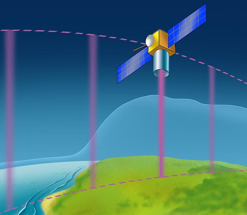
2011).Seasonal swing ranged between 20 and 35 ppm for CO2 mixing (CHUN-TA LAI, Tellus, 58B, 523–536, 2006). Studies about current spatial and temporal variations of CO2 in forest canopies provide critical information about how well a forest is coupled to the convective boundary layer (CBL) above the canopy, and therefore how susceptible this ecosystem is to increased atmospheric CO2 (Buchmann et al., Global Change Biology, 2, 421-432, 1996). CO2 gradients between the forest floor and the top of the canopy ranged between 75 and 100 ppmv at night, compared to 10-50 ppmv during the day. Both ranges represented spring conditions when canopy leaf area development had not been completed (Buchmann et al., Global Change Biology, 2, 421-432, 1996). Despite the lack of tree foliage and understorey vegetation, it is found a 5 ppmv canopy gradient during the day, but an average 23 ppmv gradient at night. (Buchmann et al., Global Change Biology, 2, 421-432, 1996) During June and July, [COj] in the upper and lower canopy (3.30-14.0 m) dropped below those of the CBL, depleting canopy air by 1-2 ppmv in June, and by 4-11 ppmv in July. Lowest canopy CO2 were reached in July, before they Increased again in fall (Buchmann et al., Global Change Biology, 2, 421-432, 1996).
Pinus        Populus        Red Butte
                  contorta    Tremuloides   Canyon Acer spp

Canopy height      13-15 m       9-13 m        13-15 m

(Buchmann et al., Global Change Biology, 2, 421-432, 1996)
As clearly reported in the IPCC fifth Assessment Report, CO2 emissions are already producing destructive effects to the plant ecosystem through the alteration of soil-atmosphere interaction mechanisms. Although the space and ground network for CO2 monitoring has regularly expanded over the past 50 years, it does not guarantee the necessary spatial and temporal resolution needed for a quantitative analysis of sources and sinks. For the purpose of estimating forests’ carbon capturing capabilities, accurate measurements of CO2 gradients between the forest floor and the top of the canopy, which ultimately translates into the capability to measure CO2 concentration profiles. Space sensors provide CO2 measurements above forest canopies, which do not allow to properly estimate Gross Primary Production (GPP). These observational gaps could be addressed with an active remote sensing system in space based on the roto-vibrational Raman lidar technique. CO2 profile measurements are possible, together with simultaneous measurements of the temperature and water vapour mixing ratio profile and a variety of additional variables (aerosol backscatter profile, aerosol extinction profile, PBL depth, cloud top and base heights, cloud optical depth). An assessment of the expected performance of the system has been performed based on the application of an analytical simulation model developed at University of Basilicata.
Space sensors provide CO2 measurements
above forest canopies, which do not allow to
properly estimate the Gross Primary Production
(GPP).

  • The estimated amount of carbon dioxide
    (CO2) in the atmosphere is equivalent to an
    amount of carbon of 8×10¹⁴ kg, while the
    amount stored in terrestrial biomass is
    5×10¹⁴ kg, 60% of which (3×10¹⁴ kg) being
    stored in forest systems.
N is the number of atoms number vibrations. The same holds true for linear molecules, however the equations 3N-5 is used, because a linear molecule has one less rotational degrees of freedom. (For a more detailed explanation see: Normal Modes). Figure 1 shows a diagram for a vibrating diatomic molecule. The levels denoted by vibrational quantum numbers v represent the potenital energy for the harmonic (quadratic) oscillator. The transition 0→10→1 is fundamental, transitions 0→n0→n (n>1) are called overtones, and transitions 1→n1→n (n>1) are called hot transitions (hot bands).
a observational requirements have to be
properly assessed.
CO2 vertical variability
The seasonal and annual mean of CO2 vertical profile reflect the combined influences of surface
fluxes and atmospheric mixing. In the Northern Hemisphere, during the summer season, midday
atmospheric CO2 concentrations are generally lower near the surface than in the free troposphere,
reflecting the higher impact of terrestrial photosynthesis over industrial emissions [5].
Conversely, during the winter, respiration and fossil-fuel sources lead to elevated low-altitude
atmospheric CO2 concentrations. The gradients are comparable in magnitude in both seasons, but
the positive gradients persist for a larger portion of the year, leading to annual-mean gradients
also showing higher atmospheric CO2 concentrations near the surface than aloft [5]. The average
midday differences in the Northern Hemisphere between 1 and 4 km, expressed in terms of CO2
mixing ratio, is –2.2 ppm in summer, +2.6 ppm in winter, while instantaneous differences may be
as large as 5-10 % [9]. The Southern Hemisphere locations show relatively constant CO2 profiles
in all seasons, with slightly higher values in the free troposphere [5]. Similar gradients are found
in the NOAA’s Carbon Tracker version 2010 [4]. CO2 gradients between the forest floor and the
top of the canopy range between 75 and 100 ppm at night, compared to 10-50 ppm during the
day. Both ranges represented spring conditions when canopy leaf area development is not
completed [10].
The central wavelength of the CO2 band is almost coincident with the twenty-first anti-Stokes
roto-vibrational O2 line, which represents a potential source of contamination for CO2 Raman
lidar measurements [11]. Riebesell [6] and Ansmann et al. [7] came to the conclusion that CO2
Raman lidar measurements were hardly feasible due to the difficulties in accurately estimating
the magnitude of the interference by O2 rotational lines. These authors also argued that
fluorescence generated by either the receiver optics or atmospheric particles could potentially
prevent from reaching a measurement accuracy at the 1 ppm level.
However, these early research efforts were conducted using excimer laser sources (Xe:Cl
mixture), which have an emission spectrum typically spanning over a spectral interval of ~0.4
nm. Such broad spectrum makes separation of CO2 and O2 lines more difficult with respect to
what is presently achievable based on the use of narrowband interference filters (0.1 nm) and
injection-seeded Nd:YAG laser sources (typical spectral width of ~0.01 nm). Whiteman et al.
[11] demonstrated that the bias affecting CO2 measurements as a result of the contamination by
the 21st O2 rotational line is not exceeding 1 % if a 0.1-nm wide IF and a narrow-band Nd:YAG
laser source (
Observational requirements for CO2 profiling - continuation
The average Northern Hemisphere midday differences between altitudes of 1 and 4 km is
–2.2 ppm in summer, +2.6 ppm in winter, and +0.7 ppm in annual mean.

The Southern Hemisphere locations show relatively constant CO2 profiles in all seasons,
with slightly higher values in the free troposphere.

Similar gradients are found in the NOAA’s (National
Oceanic and Atmospheric Administration) Carbon Tracker
version 2010 (CT2010).
An assessment of the expected performance of
the system has been performed based on the
application of an analytical simulation model
developed at University of Basilicata.
Fermi resonance results in the splitting of two vibrational bands that have nearly the same
energy and symmetry in both IR and Raman spectroscopies. The two bands are usually a
fundamental vibration and either an overtone or combination band.

As a result, two strong bands are observed in the spectrum, instead of the expected strong
and weak bands. It is not possible to determine the contribution from each vibration
because of the resulting mixed wave function.
Sistema lidar Raman per la misura
  dei profili verticali in atmosfera
del rapporto di mescolamento dell’
        anidride carbonica
For linear molecules, however the equation
3N-5 is used, because a linear molecule has
one less rotational degrees of freedom.
The Q branches of the Raman bands
associated to the
2ν1:4ν02:ν1+2ν02 Fermi resonance of 12C 16O2 ha
ve been observed in the gas phase at 2543,
2671, and 2797 cm−1 and, in addition, at 2514
cm−1,• Alternative option: Alexandrite laser source
(BeAl2O4 doped with active chromium ions,
Cr3+)
• Main advantages:
increase of laser gain with temperature which
considerable simplifies laser cooling demands.
Tuneability between 730-780 nm so that desired
wavelength can be reached by frequency-doubling (2-
times larger efficiency than frequency-tripling)
pumped by diode lasers operating in the 500-650-nm
region which are now commercially available with
high power.Although the space and ground network for CO2 monitoring has regularly expanded over the past 50 years, it does not guarantee the necessary spatial and temporal resolution needed for quantitative analysis of sources and sinks.
• The missing balance between the carbon
  released in the atmosphere through the
  combustion of fossil fuels and deforestation
  on one side, and the uptake by sinks in
  oceanic and terrestrial systems on the other
  side is responsible for the 2 ppm increasing
  rate in atmospheric CO2 concentration.
A proper definition of the CO2 observational requirements impose the assessment of CO2
time and space (vertical and horizontal) varibility
to ultimately define:
• vertical and horizontal resolution of measurements,
• measurement precision (RMS) and accuracy (bias)

                     but the positive gradients persist for a greater
                     portion of the year and the annual-mean
                     gradients also show higher atmospheric CO2
                     concentrations near the surface than aloft
                     (Stephens et al., 2007),

                   , with the only exception of the vertical region
                   from the forest floor to the top of the canopy
                   where uncertainty is 7 % (or 25 ppm) and 135
                   % (or 470 ppm), respectively
      The three fundamental vibrations of CO2 are
      v1= 1337 cm-1, v2=667 cm-1, v3=2349 cm-1.
You can also read