Reclip:century 1 Research for Climate Protection: Century Climate Simulations ACRP Project Number: A760437
←
→
Page content transcription
If your browser does not render page correctly, please read the page content below
reclip:century 1 – Uncertainty Assessment

                            reclip:century 1
               Research for Climate Protection:
                  Century Climate Simulations
                              ACRP Project Number: A760437

Expected Climate Change
and its Uncertainty in the
           Alpine Region
                          WEGC Report to ACRP Nr. 02/2011

                                               Georg Heinrich, Andreas Gobiet

                                               Wegener Center for Climate and Global Change and
                                               Institute for Geophysics, Astrophysics, and Meteor-
                                               ology/Institute of Physics,
Final Report, Part D                           University of Graz, Austria

                                               July 2011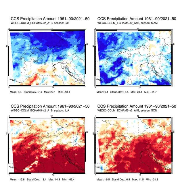
reclip:century 1 – Expected Climate Change and its Uncertainty in the Alpine Region

reclip:century -
regional climate scenarios
for the Greater Alpine Region
Funded by the Austrian Climate Research Program (ACRP)
Klima- und Energiefonds der Bundesregierung
Project number A760437

Duration: October 2008 until May 2011

Project coordinator
AIT - Austrian Institute of Technology GmbH

Project partners:
Institute of Meteorology, BOKU Wien
Wegener Center for Climate and Global Change, Graz University
Zentralanstalt für Meteorologie und Geodynamik

Georg Heinrich, Andreas Gobiet

Final Report,

Part D: Uncertainty Assessment of the reclip:century Ensemble

Wegener Center for Climate and Global Change
Graz, July 2011

                                                 2
Content
Preface................................................................................................................................................. 4

1.      Introduction................................................................................................................................ 5

2.      Uncertainties in Climate Change Projections............................................................................. 5

2.1         Natural Variability .................................................................................................................. 6

2.2         Climate Model Uncertainty.................................................................................................... 7

2.3         Emission Scenario Uncertainty .............................................................................................. 8

2.4         Downscaling uncertainty ....................................................................................................... 9

2.5         Model Weighting and Model Independence ......................................................................... 9

3.      Data and Methods.................................................................................................................... 10

3.1         Regional Climate Model Simulations ................................................................................... 10

3.2         Missing Value Reconstruction and Analysis of Variance ..................................................... 11

3.3         Representation of Uncertainty ............................................................................................ 13

4.      Results ...................................................................................................................................... 14

4.1         2-m Air Temperature ........................................................................................................... 14

4.2         Precipitation Amount........................................................................................................... 16

4.3         Summary .............................................................................................................................. 17

Annex I: IPCC Emission Scenarios...................................................................................................... 20

Annex II: Figures ................................................................................................................................ 22

References......................................................................................................................................... 45
Preface

Project goal and approach
The project reclip:century develops an ensemble of regionalized climate scenarios with 10x10 km
grid spacing until 2050 (project phase 1) and 2100 (project phase 2) for Austria and the entire
Greater Alpine Region with the aim to provide input data for climate change impact investigations.
The project is conducted in two phases. By May 2011 the project phase 1 was completed. The simu-
lation covers the period 1960 to 2000 (for validation) and future scenarios until 2050. Project phase 2
will extend the simulations till 2100 and add a scenario with higher GHG concentrations.

Project team
The project is coordinated by the Austrian Institute of Technology (AIT), project partners are the In-
stitute of Meteorology of the University of Agricultural Sciences (BOKU-Met), the Wegener Center for
Global and Climate Change (WEGC) at the University of Graz, and the Central Institute for Meteorol-
ogy and Geodynamics (ZAMG).

Report content
The complete final report (available via the project homepage http://reclip.ait.ac.at/reclip_century/)
is divided into sections according to the work package structure of the project. Below one finds the
content of the entire report.

Introduction (AIT)
A.     Models, Data and Greenhouse Gas Scenarios(AIT)
B.     Validation, Model Error Assessment (BOKU-Met, ZAMG)
B.1    Preparation observation data
B.2    Validation Temperature
B.3    Validation Radiation
B.4    Validation Precipitation
C.     Climate Scenarios - Comparative Analysis (AIT)
       ECHAM5/CCLM/A1B (WegCenter), HADCM3/CCLM/A1B (AIT)
       ECHAM5/ CCLM/B1 (ZAMG), ECHAM5/MM5/A1B (BOKU-met) – delivered in Oct.2011
D.     Expected Climate Change and its Uncertainty in the Alpine Region (WEGC, this report)
E.     Data Warehouse (AIT)

Wolfgang Loibl (AIT)
Project Coordinator

                                                  4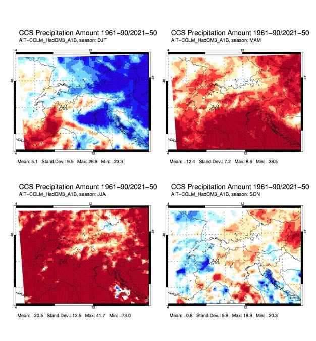
reclip:century 1 – Expected Climate Change and its Uncertainty in the Alpine Region

    1. Introduction
Regional climate simulations are subject to different sources of uncertainty stemming from the natu-
ral variability of the climate system, from emission scenarios, from errors and simplifications in the
global climate models (GCMs), and from the downscaling process with regional climate models
(RCMs).

Uncertainties can be assessed by analysing an ensemble of climate simulations which adequately
samples the various sources of uncertainty. In this report, we assess the uncertainty of the high reso-
lution climate simulations for the Alpine region produced in reclip:century 1 (see reclip:century re-
port part A) by putting them into the context of the most recent and most comprehensive ensemble
of regional climate simulations for Europe from the EU FP6 Integrated Project ENSEMBLES
(http://www.en-sembles-eu.org/). Furthermore, the relative contribution of GCMs and RCMs to total
uncertainty is investigated by a balanced analysis of variance (ANOVA).

The report is structured as follows: In Section 2 we describe the four major uncertainty sources in
climate scenarios and issues related to the construction of suitable ensembles for uncertainty analy-
sis. In Section 3 we introduce the data and methods, in Section 4 we present the results, and in Sec-
tion 5 we summarize the key findings. Parts of the analysis summarised in this report have been pub-
lished in more detail in the article by Prein et al [2011].

    2. Uncertainties in Climate Change Projections
Uncertainty in regional climate projections can be roughly divided into four components: Natural
variability, uncertainty in external forcing (mainly anthropogenic forcing due to emission of green-
house gases and land use change), uncertainty due to imperfect simulation of the climate system
(model uncertainty), and downscaling uncertainty. While model and downscaling uncertainty from
RCMs is the focus of this report and will be addressed in more detail in Section 4, we describe here
the other major uncertainty components as well. Prein et al. (2011) analysed the relative contribu-
tions of natural variability, emission scenarios and models to total uncertainty over Europe. Figure 1
gives an overview of the results and indicates the relative importance of each component. The uncer-
tainty components due to internal variability, model formulation, and emission scenario for air tem-
perature and precipitation amount over Europe until the mid and the end of the 21st century are
regarded in this study which is based on 23 different GCMs and comprises 84 simulations of the
CMIP3 ensemble. They found that uncertainty due to the formulation of the climate models is largest
for both parameters (Figure 1).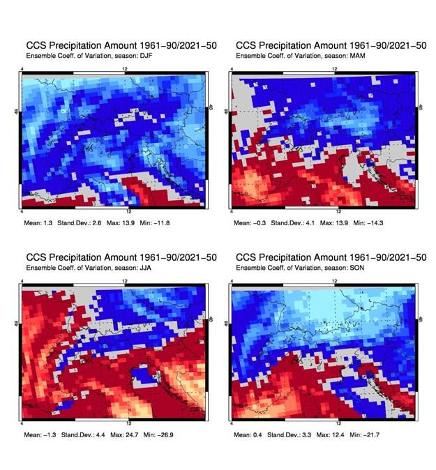
reclip:century 1 – Expected Climate Change and its Uncertainty in the Alpine Region

    Figure 1 Uncertainty components of 2-m air temperature (upper panel) and precipitation amount
                                       st
    (lower panel) for the mid of the 21 century (2021–2050 minus 1971–2000, panels a and c) and for
                       st
    the end of the 21 century (2071–2100 minus 1971–2000, panels b and d). Panels a and b show the
    fractional contribution of each uncertainty component, while panels c and d display the absolute
    values of variance. In panel c and d, the standard deviation (SD) is quoted above the bars. Source:
    Prein et al. (2011).

    2.1 Natural Variability
The term natural variability refers to deterministic and random fluctuations in the climate system,
that occur on various spatial and temporal scales. Ghil (2002) differentiates three types of phenom-
ena which cause natural variability of the climates system: (1) Variations that are directly driven by
purely periodic external forcings such as the seasonal or diurnal cycle of insolation. (2) Variations due
to the non-linear interplay of feedbacks within the climate system such as the increase of CO2 in the
atmosphere which increases surface air temperature through the greenhouse effect. The surface
warming then interacts and affects the CO2 concentration of the atmosphere directly or indirectly
through various feedback loops. (3) Variations associated with random fluctuations in physical or
chemical factors such as aerosol emissions through volcanic eruptions or weather.

Although the shorter-term weather fluctuations are of chaotic nature, they are of minor relevance on
the long term climate time scales. Since many of these chaotic variations average out on longer peri-
ods, natural variability has a larger influence on shorter than on longer averaging periods.

Uncertainty due to natural variability is typically estimated by starting and running a dynamical cli-
mate model several times with slightly different initial conditions. The difference between the results
                                                    6
reclip:century 1 – Expected Climate Change and its Uncertainty in the Alpine Region

    Figure 2 Changes in 2-m air temperature over Europe until 2100 with respect to the reference period
    1971–2000 of 23 CMIP3 global climate models under the A1B emission scenario. The thick black line
    represents the multi-model mean (from Prein, 2009).

of such experiments quantifies internal variability of the model. Since dynamical climate models are
simplified three dimensional mathematical representations of the climate system, involving its most
important components (atmosphere, ocean, land surface, and cryosphere) and allowing interactions
and feedbacks between them, internal model variability can be regarded as a measure of uncertainty
due to natural climate variability. However, uncertainties remain since it is not possible to model
future variations in solar radiation or aerosol input from volcanic eruptions. For 30-year average cli-
mate over Europe, the contribution of internal variability to total uncertainty in climate simulations
ranges from 5 % to 25 %, depending on season and meteorological parameter (Figure 1, Prein et al.,
2011). These values are strongly dependent on the length of the averaging period and are signifi-
cantly higher for single decades (e.g., Ref Hawkins and Sutton, 2009; 2011).

    2.2 Climate Model Uncertainty
Uncertainties due to climate models arise from incomplete understanding and simplified formulation
of climate processes in the models (Stainforth, 2007). In order to quantify these uncertainties, en-
sembles of different or modified climate models are used. Uncertainty related to non-physical model
parameters, which are used in parameterization schemes to describe the bulk effect of sub-grid scale
processes, can be explored by simulations with one model but different parameter choices (per-
turbed physics ensemble, PPE). Structural model uncertainty can be estimated by applying different
models with different structural design. For example, climate models can differ in the number of
climate processes which they describe, and even if they describe the same processes, different
parameterisation schemes may be applied. Hence, an ensemble of different climate models (multi-
model ensemble, MME), can be used to quantify structural uncertainties arising from different cli-

                                                    7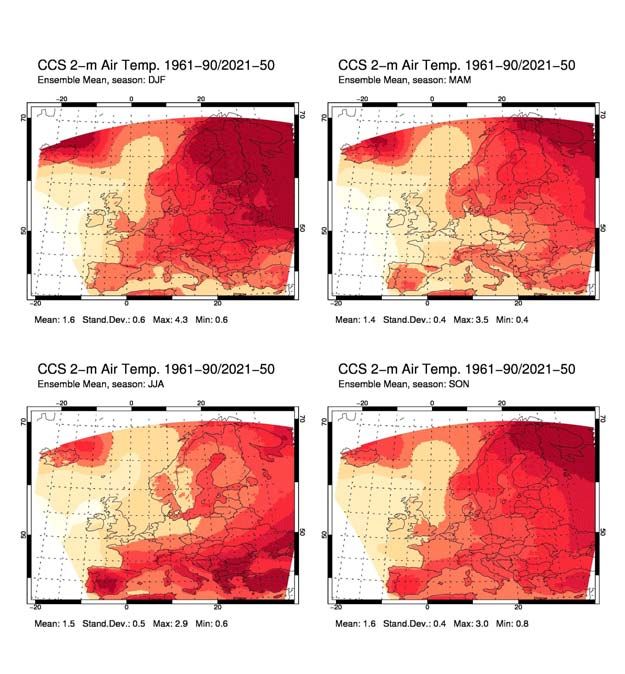
reclip:century 1 – Expected Climate Change and its Uncertainty in the Alpine Region

    Figure 3 Changes in 2-m air temperature over Europe until 2100 with respect to the reference period
    1971–2000 of 23 CMIP3 global climate models under the B1, A1B and A2 emission scenario (from
    Prein, 2009).

mate models together with parameter uncertainty. Figure 2 shows the temporal evolution of 2-m air
temperature over Europe until the end of the 21st century of 23 global climate models under the A1B
emission scenario with respect to the present-day climate, provided by the Program for Climate
Model Diagnostics and Intercomparison (PCMDI) and further referred to as CMIP3 ensemble (Meehl
et al., 2007). Although all models indicate warming, the spread of projected temperature rise until
the end of the 21st century is substantial and ranges from +1.8 K to +4.4 K (Prein, 2009). Since the
ensemble consists of different models started from different initial conditions, this range implicitly
includes natural variability along with model uncertainty. However, model uncertainty is dominant
and contributes between 45 % and 85 % to overall uncertainty in 30-year averages, depending on
lead time, season, and meteorological parameter (Figure 1, Prein et al., 2011).

    2.3 Emission Scenario Uncertainty
GHG emissions depend on many factors including population, cultural and social interactions, envi-
ronmental and economic structures, and technological development. Since it is impossible to strictly
predict the future development of these factors, the pathway of future emissions remains uncertain.
The IPCC Special Report on Emission Scenarios (SRES) (Nakicenovic et al., 2000) provides different
storylines of how the world might develop and the associated trajectory of future GHG emissions. A
description of the emission scenarios can be found in Annex I. Forcing a climate model with different
emission scenarios enables the quantification of the according uncertainty range. Figure 3 shows the
uncertainty associated with the choice of three different GHG emission scenarios (B1, A1B, and A2) .
Higher emissions result in considerable stronger warming over Europe until the end of the 21st cen-
tury, but the difference is relatively small until the mid of the 21st century. This can be partly related

                                                    8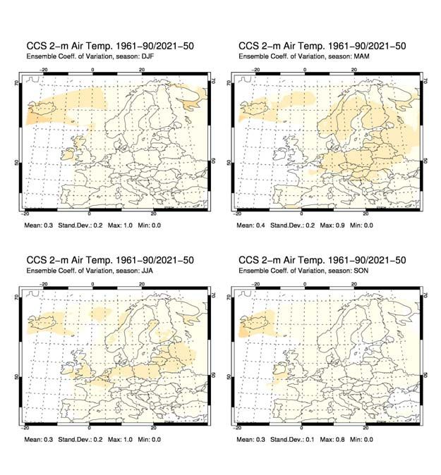
reclip:century 1 – Expected Climate Change and its Uncertainty in the Alpine Region

to the thermal inertia of the climate system and the long atmospheric lifetime of CO2 (Murphy et al.,
2009). The relative contribution of emission scenario to overall uncertainty until the mid of the 21st
century is very small (below 6 %) for both air temperature and precipitation amount. Until the end of
the 21st century, this fraction increases for air temperature to about 35 %, but remains very small for
precipitation (Figure 1, Prein et al., 2011).

    2.4 Downscaling uncertainty
GCMs operate nowadays on lattices of at about 100 km – 300 km horizontal grid spacing. Processes
related to smaller spatial scales cannot be resolved directly and therefore have to be parameterized.
Such simplifications limit the ability of GCMs to simulate effects of regional climate forcings such as
regional topography, land use, land-sea contrasts, or regional soil characteristics. Therefore, GCM
output is not representative for climate conditions at specific locations. For the analysis of regional to
local impacts of climate change additional downscaling is required.

Dynamical downscaling refers to the application of RCMs (e.g., Giorgi and Mearns, 1999), which have
the same functionality as GCMs, but are applied on limited areas and are constrained by lateral
boundary conditions (LBCs) from driving GCMs. RCMs can be operated with higher spatial resolution
than GCMs at the same computational cost. Additional regional information within the RCM domain
is introduced by regional forcings such as higher resolved orography, land-use, soil information, or
land-sea contrasts.

Downscaling methodologies such as RCMs carry their own methodological uncertainties. Déqué et al.
(2007, 2011) compared the share of uncertainty between RCMs and GCMs over Europe and found
that RCMs usually contribute a significant, but smaller part (except for precipitation in summer,
where RCMs contribute slightly over 50 %). A more comprehensive analysis of downscaling uncer-
tainty including also empirical-statistical downscaling (e.g., Benestad et al., 2009) is currently not
available.

    2.5 Model Weighting and Model Independence
In order to estimate the uncertainty of climate projections, suitable climate simulations have to be
combined and analysed with regard to their variability within the ensemble. However, the combina-
tion of different simulations is not straightforward. One of the unresolved issues in this context is
whether climate models should be weighted based on their performance in present-day climate.
Recent studies showed that there exists no single climate model which performs best across all cli-
mate variables (e.g. IPCC, 2001; Lambert and Boer, 2001). So far, there is no consensus about suit-
able performance metrics and the choice of the metric is often subjective and pragmatic (Tebaldi and

                                                    9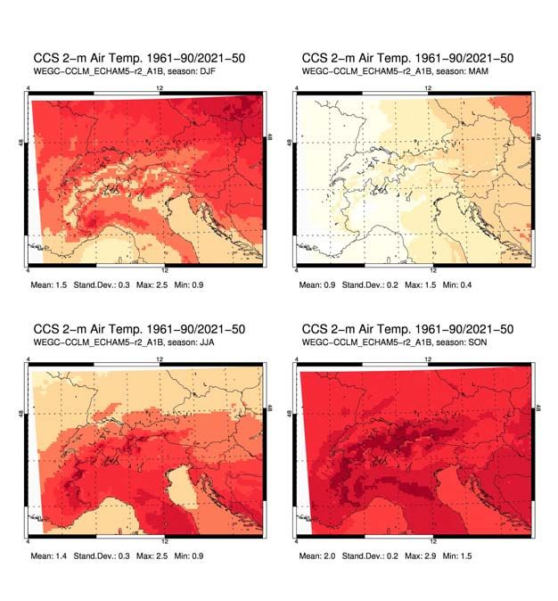
reclip:century 1 – Expected Climate Change and its Uncertainty in the Alpine Region

Knutti, 2007). In IPCC (2010), it is recommended to apply metrics which are likely to be important in
determining future climate change (e.g., metrics evaluating the simulation of key climate feedback
processes). However, such performance metrics yet have to be defined. Until now, only a few studies
indicate the potential of performance metrics to constrain the uncertainty of future climate projec-
tions in specific applications (e.g. Hall and Qu, 2006; Boe et al., 2009). In most studies only a weak
statistical relation between model performance and projected climate change has been found (e.g.
Murphy et al., 2004; Knutti et al., 2006, Sanderson et al., 2008; Knutti et al., 2009) and it couldn’t yet
be clearly demonstrated that weighted model ensembles have advantages over un-weighted ensem-
bles. For this reason, and for the subjectivity involved in the selection of performance metrics, we
don’t apply any performance weighting in this study.

Another recently discussed topic is the interdependence between different climate models. Model
interdependence could result in underestimation of variability and provoke overconfident conclu-
sions on the reliability of future climate projections. In addition, duplicate information would give too
much weight to dependent simulations and, therefore, lead to a biased estimation of the expected
change. There is reason to belief that different climate models are not independent of each other,
since model construction and setup have similarities in some state-of-the-art climate models (Pirtle,
2010). For example, Pennell and Reichler (2010) investigated the CMIP3 ensemble and found that the
amount of new information diminishes in proportion as more models are included in the ensemble.
Other studies suggest that the effective sample size of the CMIP3 ensemble is dramatically smaller
than the real number of simulations (e.g. Jun et al., 2008; Knutti et al., 2009). The issue of model
independence is even more evident in an ensemble of RCMs that are partly driven by the same GCM,
as used in our study. In this study, at least parts of the independence issue are addressed by remov-
ing potential biases which are introduced by uneven weighting of GCMs as described in Section 3.2.

    3. Data and Methods

    3.1 Regional Climate Model Simulations
The mini-ensemble of RCM simulations for the Alpine region on a 10 km grid produced in re-
clip:century and described in (reclip:century report part A) consists of three CCLM simulations: AIT-
CCLM_HadCM3_A1B which is driven by the GCM HadCM3 and forced by the A1B emission scenario,
WEGC-CCLM_ECHAM5-r2_A1B which is driven by the GCM ECHAM5 run 2 and forced by the A1B
emission scenario, and ZAMG-CCLM_ECHAM5-r2_B1 which is driven by the GCM ECHAM5 run 2 and
forced by the B1 emission scenario. This mini-ensemble is supplemented by further RCM simulations
from the EU FP6 Integrated Project ENSEMBLES (http://www.ensembles-eu.org/). In ENSEMBLES a
set of 22 high resolution RCM simulations until mid of the 21st century has been produced. The simu-

                                                   10
reclip:century 1 – Expected Climate Change and its Uncertainty in the Alpine Region
Table 1 The GCM-RCM simulation matrix of the 25 km simulations until 2050 of the EU FP6 Inte-
grated Project ENSEMBLES. The orange highlighted cells are the available simulations. The values
indicate the simulated and reconstructed changes in summer air temperature for the Greater Alpine
Region.
lations have a horizontal grid spacing of about 25 km and the LBCs were provided by eight different
GCMs. Due to limited computational resources, by far not all possible GCM-RCM combinations could
be realised in the ENSEMBLES project (cf. Table 1). The simulation matrix mainly addresses uncer-
tainty in boundary condition (GCM) and RCM uncertainty (van der Linden and Mitchell, 2009). Uncer-
tainty due to natural variability is only implicitly regarded by using different GCMs. Concerning future
GHG emissions, only the A1B emission scenario (Nakicenovic et al., 2000) was used. This means, that
three of the four major uncertainty components are covered by the ensemble. A rough estimate to
which extent the overall uncertainty is underestimated by only using one emission scenario in EN-
SEMBLES can be obtained from Prein et al. (2011), who showed that emission scenario uncertainty is
small in the first half of the 21st century (see Section 2.3).
We analyse and classify the reclip:century simulations in four subregions of the Alpine area (Figure 4)
in the framework of the A1B uncertainty range spanned by the 22 ENSEMBLES simulations. This
analysis is aims at facilitating the interpretation of the reclip:century simulations and in particular to
indicate their position within the A1B uncertainty range.
3.2 Missing Value Reconstruction and Analysis of Variance
Since RCMs are constrained by GCMs at their boundaries, the issue of model independence (Section
2.5) is even more obvious and crucial for an RCM ensemble than for a GCM ensemble. This arises
from the fact that two different RCMs driven by the same GCM are obviously not independent
through the same LBCs. The GCM-RCM simulation matrix shown in Table 1 reveals that the majority
of RCMs have been forced by the two GCMs ECHAM5-r3 and HadCM3Q0 (10 out of 22 simulations).
Therefore, those two GCMs are overweighed compared to the other GCMs and ensemble mean cli-
mate change signals are potentially biased towards the climate sensitivity of these two GCMs.
To avoid biased estimates, the missing climate change signals (CCSs) of Table 1 are reconstructed
following Déqué et al. (2007). The reconstruction method is embedded in the framework of an analy-
sis of variance (ANOVA) where the highest interaction term is neglected in order to reconstruct the
11reclip:century 1 – Expected Climate Change and its Uncertainty in the Alpine Region
Figure 4 The four HISTALP regions studied: GAR-Northwest, GAR-Northeast, GAR-Southwest, and
GAR-Southeast (picture taken from http://www.zamg.ac.at/histalp/).
actual missing value. The reconstruction algorithm assumes additive factors. In case of our ensemble
only two factors are considered, namely GCM and RCM. As a simple example, consider two RCMs,
one driven by all GCMs, the other RCM driven by all GCMs except one. Then this missing value is re-
constructed by adding the mean difference between both RCMs driven by all available GCMs to the
second RCM. Since the reconstruction of the actual missing value depends on the grand mean of the
entire GCM-RCM matrix, 100 iterations are performed to reconstruct the missing values.
A leave-one-out cross validation is computed in order to analyse the skill of the reconstruction
method. Since the algorithm requires at least one element for each row and column, only eleven
GCM-RCM combinations remain for the evaluation (cf. Table 1). In order to enlarge the sample size,
the missing values are reconstructed on monthly basis and the evaluation is carried out on the
pooled seasonal values. Table 2 shows the result of the leave-one-out cross validation on seasonal
basis by comparing the original ensemble with the purely reconstructed ensemble for 2-m air tem-
perature and precipitation amount for the Greater Alpine Region (GAR) and the four HISTALP re-
gions. It can be seen that the mean CCS is well reconstructed with deviations (original minus recon-
structed) of less than 0.1 K and 2 % for air temperature and precipitation amount, respectively. For
precipitation, large relative bias values with respect to the original mean change are obtained only if
the original CCS is close to zero. Changes in the dispersion of the distribution are quantified via the
ratio of reconstructed to original standard deviation. The reconstructed distributions mostly show an
overestimation of the standard deviation and slightly better ratios are obtained for 2-m air tempera-
ture than for precipitation. These results indicate that the reconstruction algorithm provides reason-
able distributions for both parameters considering the rather simple linearity assumptions of the
reconstruction method.
12reclip:century 1 – Expected Climate Change and its Uncertainty in the Alpine Region
Table 2 Leave-one-out cross validation of the reconstruction algorithm for 2-m air temperature (up-
per table) and precipitation amount (lower table).
The reconstruction algorithm was applied to fill the missing values in the ENSEBMLES GCM-RCM
simulation matrix (Table 1). The filled matrix is further used to calculate a balanced ANOVA concern-
ing the influence of the two factors GCM and RCM in order to quantify their relative contribution to
the total uncertainty. In addition, enhanced estimates of uncertainty in the four sub-regions (see
Section 4) are based on the filled matrix.
3.3 Representation of Uncertainty
Uncertainties of the projected changes are quantified by different measures. The multi-model mean
and different percentiles are provided as measures of location. The coefficient of variation (CV) is
calculated as a normalized measure of dispersion. The CV is defined as the ratio of intermodel stan-
dard deviation to multi-model mean change. For example, a CV of 0.5 indicates that about 96 % of
the CCSs have the same sign as the multi-model mean under the assumption of normally distributed
13reclip:century 1 – Expected Climate Change and its Uncertainty in the Alpine Region
data. More generally, low CVs correspond to lower dispersion around the multi-model mean and
indicate robustness in the sign of the multi-model mean change. Since small multi-model mean val-
ues can cause unrealistically large CVs, grid points with projected precipitation changes ≤ 1 % are
neglected and the CV is not calculated.
4. Results
All figures discussed in the following section are collectively displayed in Annex II. Concerning uncer-
tainty estimates, only the map plots are based on the original ENSEMBLES GCM-RCM matrix.
4.1 2-m Air Temperature
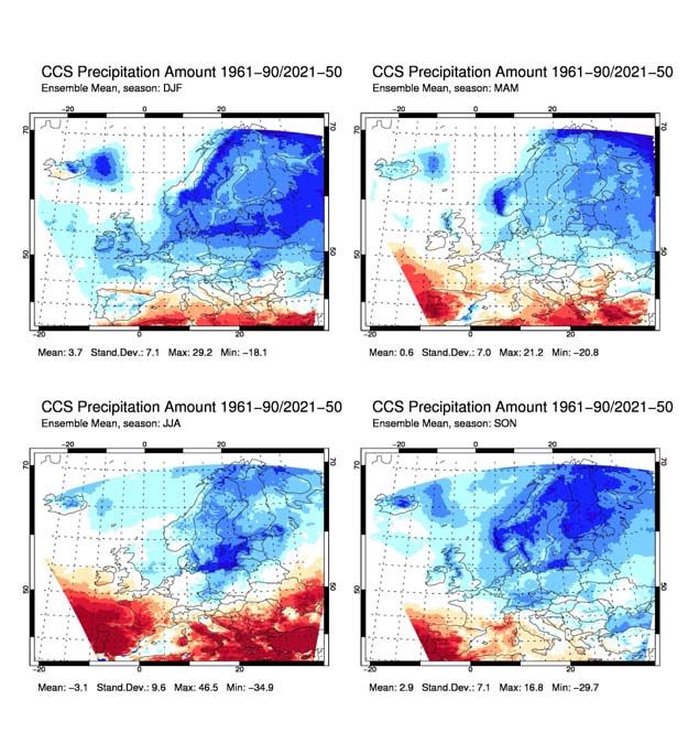
Figure 5 and Figure 7 show maps of the multi-model mean change of the original ENSEMBLES CCS
matrix over Europe and the Greater Alpine Region (GAR). The CCS is calculated as the mean differ-
ence between future period (2021-2050) and reference period (1961-1990). The projected changes
of 2-m air temperature show a positive sign in all seasons. The most responsive regions are the
north-eastern parts of Europe in winter and the southern parts of Europe in summer. The spatial
differences can be largely explained by the modest warming of the ocean, influencing the maritime
climate of western Europe in combination with altered snow-albedo feedback mechanisms in north-
ern and eastern Europe (Rowell, 2005). The high summer temperatures in the south can be related to
an earlier and more rapid reduction of soil moisture in spring (e.g. Wetherald and Manabe, 1995;
Gregory et al., 1997). The spatial averages of the multi-model mean change are seasonally varying
between +1.4 K in spring (MAM) and +1.6 K in autumn (SON) and winter (DJF). For the GAR, a
stronger warming is obtained along the Alpine ridge especially in summer (JJA). The spatial average
shows a minimum in MAM and a maximum in JJA with a warming of +1.2 K and +1.7 K, respectively.
Figure 6 and Figure 8 show the CV for the original CCS matrix over Europe and the GAR. Robust tem-
perature changes are obtained over all of Europe with CV values mostly lower than 0.5, indicating
low dispersion around the multi-model mean change.
Figure 12 to Figure 16 depict scatter plots for the unfilled ENSEMBLES CCS matrix of 2-m air tempera-
ture and precipitation amount for the GAR and the four HISTALP regions. In addition, the three re-
clip:century simulations are shown. It can be seen that temperature change in the ECHAM5-r3 driven
RCM simulations are mostly below the median of the distribution. Particularly in winter, the
ECHAM5-r3 driven simulations are at the lower bound of the distribution while for the other seasons
the CGCM3 and BCM driven RCM simulations indicate lower CCSs. In contrast, the HadCM3 simula-
tions mostly indicate larger temperature CCSs than the median of the multi-model ensemble. This is
in accordance with the projected changes of the CMIP3 ensemble shown in Figure 2 where the
14reclip:century 1 – Expected Climate Change and its Uncertainty in the Alpine Region
ECHAM5 simulation (mpi_echam5) shows lower CCSs than the HadCM3 simulation (ukmo_hadcm3).
The difference in the climate sensitivity of the driving GCMs is also subject to the three member re-
clip:century ensemble, where the CCLM simulation driven by HadCM3 (AIT_CCLM) clearly indicates
the largest CCSs for DJF, MAM, and JJA. Since the other two reclip:century simulations were driven by
ECHAM5-r2 forced with different emission scenarios (WEGC_CCLM forced by A1B and ZAMG_CCLM
forced by B1), the difference between the two simulations is mainly due to the choice of different
emission scenarios. The largest differences between the two simulations occur in DJF with larger
CCSs for WEGC_CCLM and in JJA with larger CCSs for ZAMG_CCLM. However, these differences
mostly average out in the annual mean and the A1B forced CCLM simulation reveals larger CCSs as
expected. The spatial pattern of the CCSs for the three reclip:century RCM simulations over the GAR
are shown in Figure 9 to Figure 11. In general, large differences between the simulations are ob-
tained especially at smaller spatial scales. For the GAR, the HadCM3 driven simulation AIT_CCLM
shows a maximum warming in summer with 2.6 K, while the other two ECHAM5 driven simulations
have their maximum in autumn with 2.0 K and 1.9 K for WEGC_CCLM and ZAMG_CCLM, respectively.
However, similarities are found mainly for the two ECHAM5 driven simulations with, for example, a
pronounced warming along the Alpine ridge in SON.
Figure 17 to Figure 21 depict histograms and the associated kernel density estimates of the recon-
structed ENSEMBLES CCS matrix for the GAR and the four HISTALP regions. The projected warming is
lowest in MAM for all investigated subregions, while the largest changes are obtained in DJF (JJA) in
the northern (southern) HISTALP regions. Concerning the spread of the reclip:century simulations,
the range of the reconstructed ENSEMBLES CCS matrix is better sampled in DJF and JJA than in MAM
and SON. For the GAR, the width of the histograms and the associated kernel estimates, and there-
fore the associated uncertainty, is lowest (largest) in DJF (JJA) with a difference of 1.2 K (1.5 K) be-
tween the 90th (Q.90) and 10th (Q.10) percentile of the reconstructed ENSEMBLES CCS matrix. For the
four HISTALP regions, the overall lowest (largest) uncertainty is obtained for GAR-Southwest in DJF
(GAR-Southwest in SON) with a difference of 1.2 K (1.9 K) between Q.90 and Q.10 of the recon-
structed ENSEMBLES CCS matrix. Generally large uncertainty during JJA and SON is underlined by
Figure 22 to Figure 24 which show the annual cycle and the associated uncertainty of the recon-
structed ENSEMBLES CCS matrix.
Figure 25 to Figure 27 show the results of the ANOVA for the reconstructed ENSEMBLES CCS matrix.
Again, it can be seen that the overall variation is largest in JJA and SON with standard deviations be-
tween 0.5 K and 0.7 K. The variance decomposition reveals that the choice of the GCM has the larg-
est effect on the total variation, contributing in most cases more than 70 % to the overall variance.
RCM variance contribution is largest in DJF and SON for GAR-Northwest and GAR-Southwest, indicat-
15reclip:century 1 – Expected Climate Change and its Uncertainty in the Alpine Region
ing that the choice of the RCM plays an important role in these two seasons. For GAR-Northeast and
GAR-Southeast, higher (lower) variation is introduced due to the choice of the RCM in MAM and JJA
(DJF). Here, the choice of the RCM contributes about 20-25 % and peaks up to 34.6 % in SON for
GAR-Northeast.
4.2 Precipitation Amount
Figure 5 and Figure 7 show maps of the multi-model mean change of the unfilled ENSEMBLES CCS
matrix over Europe and the GAR. The CCS is calculated as the relative difference between future and
reference period with respect to the present-day climate. The changes clearly indicate a dipolar
north-south pattern with reduced precipitation over southern Europe. Areas with reduced precipita-
tion show a northward shift from winter to summer which is identified as the European Climate
change Oscillation (ECO) and can be related to a seasonal dependent northward shift of the mid-
latitude storm track (Giorgi and Coppola, 2007). The spatial average is seasonal varying between -3.1
% in JJA and +3.7 % in DJF. For the GAR, a distinct impact of the Alpine ridge on the spatial distribu-
tion of the projected precipitation changes is obtained. For example, MAM, JJA and SON show an
increase of precipitation north of the Alps, while the southern and western parts indicate a decrease
of the multi-model mean. The spatial mean of the multi-model mean shows a minimum in summer
with -3.1 % and a maximum in winter with +3.7%.
Figure 6 and Figure 8 show the CV for the unfilled CCS matrix over Europe and the GAR. On the large
scale over Europe, robust changes are only obtained in southern and northern parts of Europe for
areas which show the most pronounced multi-model mean change. Along the transition zone from
pronounced drier conditions in the south to wetter conditions in the north the changes are highly
uncertain, indicated by CV values ≥ 2.0 for a large fraction of the domain.
Figure 12 to Figure 16 depict scatter plots for the unfilled ENSEMBLES CCS matrix of 2-m air tempera-
ture and precipitation amount for the GAR and the four HISTALP regions. In addition, the three re-
clip:century simulations are shown. It can be seen that the ECHAM5-r3 driven RCM simulations
mostly indicate positive precipitation changes in DJF while in MAM and SON the changes are mostly
located at the lower bound of the multi-model ensemble. The HadCM3 simulations mostly show
negative (positive) precipitation change signals in JJA (SON) which tend to be located at the lower
(upper) bound of the multi-model ensemble. All three reclip:century simulations indicate negative
CCSs in summer and the HadCM3 driven simulation AIT_CCLM shows the most pronounced changes.
For the other seasons, the changes of the reclip:century ensemble are more diverse and both posi-
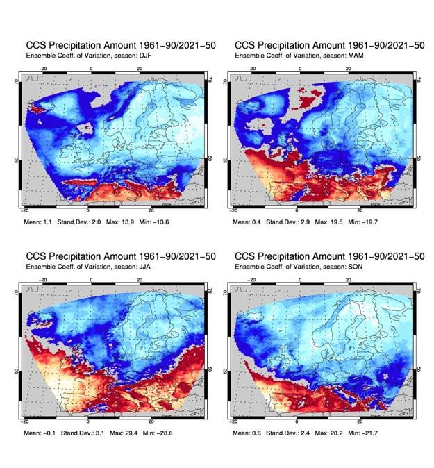
tive and negative precipitation CCSs are obtained. The spatial pattern of the CCSs for the three re-
clip:century RCM simulations over the GAR are shown in Figure 9 to Figure 11. In general, substantial
16reclip:century 1 – Expected Climate Change and its Uncertainty in the Alpine Region
differences in the spatial pattern of the precipitation changes among the simulations are obtained,
indicating the importance of sampling different driving GCMs and GHG emission scenarios. For ex-
ample, the three simulations don‘t agree in the sign of change even in the spatial average in DJF and
MAM.
Figure 17 to Figure 21 depict histograms and the associated kernel density estimates of the recon-
structed ENSEMBLES CCS matrix for the GAR and the four HISTALP regions. In most cases, the median
(Q.50) is located very close to zero in combination with large dispersion. For the GAR, GAR-
Southeast, and GAR-Southwest, the largest changes are obtained in DJF with +4.0 %, +4.7 %, and +3.7
%, respectively. For GAR-Northeast and GAR-Northwest, the largest changes are obtained in SON and
MAM with +5.1 % and +3.2 %, respectively. Concerning the spread of the reclip:century simulations,
the range of the reconstructed ENSEMBLES CCS matrix is generally better sampled in DJF and MAM
than in JJA and SON. For the GAR, the width of the histograms and the associated kernel estimates,
and therefore the associated uncertainty, is lowest (largest) in DJF (JJA) with a difference of 12.2 %
(21.3 %) between Q.90 and Q.10 of the reconstructed ENSEMBLES CCS matrix. For the four HISTALP
regions, the overall lowest (largest) uncertainty is obtained for GAR-Southwest in DJF (JJA) with a
difference of 13.8 % (30.2 %) between Q.90 and Q.10 of the reconstructed ENSEMBLES CCS matrix.
Large uncertainty of the projected changes especially in JJA and SON is also highlighted by Figure 22
to Figure 24 which show the annual cycle and the associated uncertainty of the reconstructed EN-
SEMBLES CCS matrix.
Figure 25 to Figure 27 show the results of the ANOVA for the reconstructed ENSEMBLES CCS matrix.
Again, it can be seen that the overall standard deviation is mostly largest in JJA and SON with stan-
dard deviations ranging from 7.1 % to 11.0 %. The variance decomposition reveals that the choice of
the RCM is by far more important than for 2-m air temperature. Especially in MAM and JJA the RCMs
have a larger effect on the total variation than the GCMs. Here, the choice of the RCM contributes
about 50-60 % to the total variation and peaks up to 64.9 % in JJA for GAR-Southwest, indicating that
the choice of the RCM plays the dominant role in these two seasons. In SON and DJF, the choice of
the GCM is the dominant factor and explains between 55.6 % in DJF for GAR-Southwest and 78.7 % in
SON for GAR-Northwest.
4.3 Summary
The RCM ensemble produced in reclip:century is subject to different uncertainty sources, namely
natural variability, emission scenario uncertainty, uncertainties arising from different GCMs and un-
certainties due to dynamical downscaling. We assessed the uncertainties of the reclip:century simu-
lations for air temperature and precipitation amount until the mid of the 21st century over the Alpine
17reclip:century 1 – Expected Climate Change and its Uncertainty in the Alpine Region
Region by including further RCM simulations with a coarser horizontal resolution of about 25 km
from the EU FP6 Integrated Project ENSEMBLES. This was accomplished by analysing the range of the
climate change signals of the reclip:century simulations with respect to the larger ensemble of the
ENSEMBLES project. Since the choice of the GHG emission scenario is less important until the mid of
the 21st century, only the A1B emission scenario was used to force the climate simulations in EN-
SEMBLES. The majority of RCM simulations have been forced by only two global climate models and,
therefore, an artificially caused bias of the climate change signals towards the climate sensitivity of
these two GCMs is introduced. To avoid this, the missing CCSs of the ENSEMBLES simulation matrix
were reconstructed. A leave-one-out cross validation showed that the reconstruction algorithm pro-
vides reasonable distributions for 2-m air temperature and precipitation. The reconstructed CCSs
were used to calculate a balanced ANOVA concerning the two factors GCM and RCM in order to
quantify their relative contribution to the total variance of the reconstructed GCM-RCM matrix and
to obtain an unbiased estimate of climate change over the greater Alpine region. The key findings
can be summarized as follows:
– For 2-m air temperature, a greater warming is obtained along the Alpine ridge especially in
summer and autumn. The reclip:century CCLM simulation driven by HadCM3 (AIT_CCLM)
clearly indicates the largest CCSs in DJF, MAM, and JJA. The largest differences between the
two ECHAM5-driven simulations occur in DJF with larger CCSs for WEGC_CCLM and in JJA
with larger CCSs for ZAMG_CCLM. The results of the uncertainty analysis reveal strong ro-
bustness of the projected warming in all seasons. The width of the histograms and the asso-
ciated kernel estimates, and therefore the associated uncertainty, is lowest (largest) in DJF
(JJA) with a difference of 1.2 K (1.5 K) between Q.90 and Q.10. For the four HISTALP regions,
the overall lowest (largest) uncertainty is obtained for GAR-Southwest in DJF (GAR-
Southwest in SON) with a difference of 1.2 K (1.9 K) between Q.90 and Q.10. Concerning the
spread of the reclip:century simulations, the range of the ENSEMBLES CCS matrix is better
sampled in DJF and JJA than in MAM and SON. The variance decomposition reveals that the
choice of the GCM has by far the largest effect on the total variation, contributing between
65 % and 90 % to the overall variance, dependent on season and region.
– For precipitation amount, all three reclip:century simulations indicate negative CCSs in sum-
mer and the HadCM3 driven simulation AIT_CCLM shows the most pronounced changes. For
the other seasons, the changes are more diverse and both positive and negative precipitation
CCSs are obtained. The multi-model mean of the ENSEMBLES simulations reveal a distinct
impact of the Alpine ridge on the spatial distribution of the projected changes, with an in-
crease of precipitation north of the Alps in MAM, JJA and SON while the southern and west-
18reclip:century 1 – Expected Climate Change and its Uncertainty in the Alpine Region
ern parts indicate a decrease. Along this transition the changes are highly uncertain. For the
GAR, the width of the histograms and the associated kernel estimates, and therefore the as-
sociated uncertainty, is lowest (largest) in DJF (JJA) with a difference of 12.2 % (21.3 %) be-
tween Q.90 and Q.10 of the reconstructed ENSEMBLES CCS matrix. For the four HISTALP re-
gions, the overall lowest (largest) uncertainty is obtained for GAR-Southwest in DJF (JJA) with
a difference of 13.8 % (30.2 %) between Q.90 and Q.10. Concerning the spread of the re-
clip:century simulations, the range of the ENSEMBLES CCS matrix is generally better sampled
in DJF and MAM than in JJA and SON. The variance decomposition reveals that the choice of
the RCM is by far more important than for 2-m air temperature. Particularly in MAM and JJA
the RCM contribution to the total variation is larger than that of the GCMs.
19reclip:century 1 – Expected Climate Change and its Uncertainty in the Alpine Region
Annex I: IPCC Emission Scenarios
The following description of the IPCC emission scenarios can be found in Nakićenović and Swart
(2000):
A1. The A1 storyline and scenario family describes a future world of very rapid economic growth,
global population that peaks in mid-century and declines thereafter, and the rapid introduction of
new and more efficient technologies. Major underlying themes are convergence among regions,
capacity building and increased cultural and social interactions, with a substantial reduction in re-
gional differences in per capita income. The A1 scenario family develops into three groups that de-
scribe alternative directions of technological change in the energy system. The three A1 groups are
distinguished by their technological emphasis: fossil-intensive (A1FI), non-fossil energy sources (A1T)
or a balance across all sources (A1B) (where balanced is defined as not relying too heavily on one
particular energy source, on the assumption that similar improvement rates apply to all energy sup-
ply and end use technologies).
A2. The A2 storyline and scenario family describes a very heterogeneous world. The underlying
theme is self-reliance and preservation of local identities. Fertility patterns across regions converge
very slowly, which results in continuously increasing population. Economic development is primarily
regionally oriented and per capita economic growth and technological change more fragmented and
slower than other storylines.
B1. The B1 storyline and scenario family describes a convergent world with the same global popula-
tion, that peaks in mid-century and declines thereafter, as in the A1 storyline, but with rapid change
in economic structures toward a service and information economy, with reductions in material inten-
sity and the introduction of clean and resource-efficient technologies. The emphasis is on global solu-
tions to economic, social and environmental sustainability, including improved equity, but without
additional climate initiatives.
B2. The B2 storyline and scenario family describes a world in which the emphasis is on local solutions
to economic, social and environmental sustainability. It is a world with continuously increasing global
population, at a rate lower than A2, intermediate levels of economic development, and less rapid
and more diverse technological change than in the B1 and A1 storylines. While the scenario is also
oriented towards environmental protection and social equity, it focuses on local and regional levels.
An illustrative scenario was chosen for each of the six scenario groups A1B, A1FI, A1T, A2, B1 and B2.
All should be considered equally sound.
20reclip:century 1 – Expected Climate Change and its Uncertainty in the Alpine Region
The SRES scenarios do not include additional climate initiatives, which means that no scenarios are
included that explicitly assume implementation of the United Nations Framework Convention on
Climate Change or the emissions targets of the Kyoto Protocol.
21reclip:century 1 – Expected Climate Change and its Uncertainty in the Alpine Region
Annex II: Figures
Figure 5 Multi-model mean changes in 2-m air temperature (upper panel) and precipita-
tion amount (lower panel) for the 22 ENSEMBLES simulations between 2021-2050 and
1961-1990 for Europe. Changes of precipitation amount are calculated relative with re-
spect to 1961-1990.
22reclip:century 1 – Expected Climate Change and its Uncertainty in the Alpine Region
Figure 6 Coefficient of variation of the changes between 2021-2050 and 1961-1990 for
Europe for the 22 ENSEMBLES simulations for 2-m air temperature (upper panel) and
precipitation amount (lower panel). Changes of precipitation amount are calculated rela-
tive with respect to 1961-1990.
23reclip:century 1 – Expected Climate Change and its Uncertainty in the Alpine Region
Figure 7 Multi-model mean changes in 2-m air temperature (upper panel) and precipita-
tion amount (lower panel) for the 22 ENSEMBLES simulations between 2021-2050 and
1961-1990 for the GAR. Changes of precipitation amount are calculated relative with re-
spect to 1961-1990.
24reclip:century 1 – Expected Climate Change and its Uncertainty in the Alpine Region
Figure 8 Coefficient of variation of the changes between 2021-2050 and 1961-1990 for the
GAR for the 22 ENSEMBLES simulations for 2-m air temperature (upper panel) and precipi-
tation amount (lower panel). Changes of precipitation amount are calculated relative with
respect to 1961-1990.
25reclip:century 1 – Expected Climate Change and its Uncertainty in the Alpine Region
Figure 9 Changes of 2-m air temperature (upper panel) and precipitation amount (lower
panel) for the AIT_CCLM between 2021-2050 and 1961-1990 for the GAR. Changes of
precipitation amount are calculated relative with respect to 1961-1990.
26reclip:century 1 – Expected Climate Change and its Uncertainty in the Alpine Region
Figure 10 Changes of 2-m air temperature (upper panel) and precipitation amount (lower
panel) for the WEGC_CCLM between 2021-2050 and 1961-1990 for the GAR. Changes of
precipitation amount are calculated relative with respect to 1961-1990.
27reclip:century 1 – Expected Climate Change and its Uncertainty in the Alpine Region
Figure 11 Changes of 2-m air temperature (upper panel) and precipitation amount (lower
panel) for the ZAMG_CCLM between 2021-2050 and 1961-1990 for the GAR. Changes of
precipitation amount are calculated relative with respect to 1961-1990.
28reclip:century 1 – Expected Climate Change and its Uncertainty in the Alpine Region
Figure 12 Scatter plots for the changes in 2-m air temperature and precipitation amount between 2021-2050
and 1961-1990 for the GAR for the 22 ENSEMBLES simulations. Changes of precipitation amount are calculated
relative with respect to 1961-1990. The black lines indicate the median changes.
29reclip:century 1 – Expected Climate Change and its Uncertainty in the Alpine Region
Figure 13 Scatter plots for the changes in 2-m air temperature and precipitation amount between 2021-2050
and 1961-1990 for GAR-Northwest for the 22 ENSEMBLES simulations. Changes of precipitation amount are
calculated relative with respect to 1961-1990. The black lines indicate the median changes.
30reclip:century 1 – Expected Climate Change and its Uncertainty in the Alpine Region
Figure 14 Scatter plots for the changes in 2-m air temperature and precipitation amount between 2021-2050
and 1961-1990 for GAR-Northeast for the 22 ENSEMBLES simulations. Changes of precipitation amount are
calculated relative with respect to 1961-1990. The black lines indicate the median changes.
31reclip:century 1 – Expected Climate Change and its Uncertainty in the Alpine Region
Figure 15 Scatter plots for the changes in 2-m air temperature and precipitation amount between 2021-2050
and 1961-1990 for GAR-Southwest for the 22 ENSEMBLES simulations. Changes of precipitation amount are
calculated relative with respect to 1961-1990. The black lines indicate the median changes.
32reclip:century 1 – Expected Climate Change and its Uncertainty in the Alpine Region
Figure 16 Scatter plots for the changes in 2-m air temperature and precipitation amount between 2021-2050
and 1961-1990 for GAR-Southeast for the 22 ENSEMBLES simulations. Changes of precipitation amount are
calculated relative with respect to 1961-1990. The black lines indicate the median changes.
33reclip:century 1 – Expected Climate Change and its Uncertainty in the Alpine Region
Figure 17 Histograms and kernel density estimates of the reconstructed changes in 2-m air temperature
(upper panel) and precipitation amount (lower panel) between 2021-2050 and 1961-1990 for the GAR.
Changes of precipitation amount are calculated relative with respect to 1961-1990. The dashed lines
represent Q.10, Q.50, and Q.90.
34reclip:century 1 – Expected Climate Change and its Uncertainty in the Alpine Region
Figure 18 Histograms and kernel density estimates of the reconstructed changes in 2-m air temperature
(upper panel) and precipitation amount (lower panel) between 2021-2050 and 1961-1990 for GAR.-
Northwest Changes of precipitation amount are calculated relative with respect to 1961-1990. The
dashed lines represent Q.10, Q.50, and Q.90.
35reclip:century 1 – Expected Climate Change and its Uncertainty in the Alpine Region
Figure 19 Histograms and kernel density estimates of the reconstructed changes in 2-m air temperature
(upper panel) and precipitation amount (lower panel) between 2021-2050 and 1961-1990 for GAR-
Northeast. Changes of precipitation amount are calculated relative with respect to 1961-1990. The
dashed lines represent Q.10, Q.50, and Q.90.
36reclip:century 1 – Expected Climate Change and its Uncertainty in the Alpine Region
Figure 20 Histograms and kernel density estimates of the reconstructed changes in 2-m air temperature
(upper panel) and precipitation amount (lower panel) between 2021-2050 and 1961-1990 for GAR-
Southwest. Changes of precipitation amount are calculated relative with respect to 1961-1990. The
dashed lines represent Q.10, Q.50, and Q.90.
37reclip:century 1 – Expected Climate Change and its Uncertainty in the Alpine Region
Figure 21 Histograms and kernel density estimates of the reconstructed changes in 2-m air temperature
(upper panel) and precipitation amount (lower panel) between 2021-2050 and 1961-1990 for GAR-
Southeast. Changes of precipitation amount are calculated relative with respect to 1961-1990. The
dashed lines represent Q.10, Q.50, and Q.90.
38reclip:century 1 – Expected Climate Change and its Uncertainty in the Alpine Region
Figure 22 Annual cycle of the reconstructed CCSs in 2-m air temperature (upper panel) and precipita-
tion amount (lower panel) between 2021-2050 and 1961-1990 for the GAR Changes of precipitation
amount are calculated relative with respect to 1961-1990.
39reclip:century 1 – Expected Climate Change and its Uncertainty in the Alpine Region
Figure 23 Annual cycle of the reconstructed changes in 2-m air temperature and precipitation amount between
2021-2050 and 1961-1990 for GAR-Northeast (upper panel) and GAR-Northwest (lower panel). Changes of precipitation
amount are calculated relative with respect to 1961-1990.
40reclip:century 1 – Expected Climate Change and its Uncertainty in the Alpine Region
Figure 24 Annual cycle of the reconstructed changes in 2-m air temperature and precipitation amount between
2021-2050 and 1961-1990 for GAR-Southeast (upper panel) and GAR-Southwest (lower panel). Changes of precipitation
amount are calculated relative with respect to 1961-1990.
41reclip:century 1 – Expected Climate Change and its Uncertainty in the Alpine Region
Figure 25 Analysis of variance of the reconstructed changes in 2-m air temperature (upper panel) and
precipitation amount (lower pannel) between 2021-2050 and 1961-1990 for the GAR. Changes of
precipitation amount are calculated relative with respect to 1961-1990.
42reclip:century 1 – Expected Climate Change and its Uncertainty in the Alpine Region
Figure 26 Analysis of variance of the reconstructed changes in 2-m air temperature and precipitation amount between
2021-2050 and 1961-1990 for GAR-Northeast (upper panel) and GAR-Northwest (lower panel). Changes of precipitation
amount are calculated relative with respect to 1961-1990.
43reclip:century 1 – Expected Climate Change and its Uncertainty in the Alpine Region
Figure 27 Analysis of variance of the reconstructed changes in 2-m air temperature and precipitation amount between
2021-2050 and 1961-1990 for GAR-Southeast (upper panel) and GAR-Southwest (lower panel). Changes of precipitation
amount are calculated relative with respect to 1961-1990.
44reclip:century 1 – Expected Climate Change and its Uncertainty in the Alpine Region
References
Benestad RE, Hanssen-Bauer I, Chen D. 2009. Empirical Statistical Downscaling. World Scientific Pub-
lishing Company, New Jersey, London
Boe JL, Hall A, Qu X. 2009: September sea-ice cover in the Arctic Ocean projected to vanish by 2100.
Nat. Geosci., 2: 341-343.
Déqué M, Rowell DP, Lüthi D, Giorgi F, Christensen JH, Rockel B, Jacob D, Kjellström E, de Castro M,
van den Hurk B. 2007. An intercomparison of regional climate simulations for Europe: assessing un-
certainties in model projections. Climatic Change 81: 53–70. DOI: 10.1007/s10584-006-9228-x.
Dobler A, Ahrens B. 2008. Precipitation by a regional climate model and bias correction in Europe and
South Asia. Meteorologische Zeitschrift 17: 499─509.
Frei C, Christensen JH, Déqué M, Jacob D, Jones RG, Vidale PL. 2003. Daily precipitation statistics in
regional climate models: Evaluation and intercomparison for the European Alps. Journal of Geo-
physical Research 108 (D3), 4124. DOI:10.1029/2002JD002287.
Giorgi F, Coppola E. 2007. European climate-change oscillation (ECO). Geophysical Research Letter
34: L21703. DOI:10.1029/2007GL031223.
Giorgi, F, Mearns LO. 1999. Introduction to special section: Regional climate modeling revisited, J.
Geophys. Res., 104, 6335-6352, 1999.
Ghil M. 2002. Natural Climate Variability in Encyclopedia of Global Environmental Change, Volume 1,
The Earth System: Physical and Chemical Dimensions of Global Environmental Change. John Wiley
& Sons, Ltd: Chichester.
Gregory JM, Mitchell JFB, Brady AJ. 1997. Summer Drought in Northern Midlatitudes in a Time-
Dependent CO2 Climate Experiment. Journal of Climate 10: 662–686
Hagemann S, Machenhauer B, Jones R, Christensen OB, Déqué M, Jacob D, Vidale PL. 2004. Evalua-
tion of Water and Energy Budgets in Regional Climate Models Applied Over Europe. Climate Dy-
namics 23: 547─567.
Hall A, Qu X. 2006. Using the current seasonal cycle to constrain snow albedo feedback in future cli-
mate change. Geophys. Res. Lett. 33. DOI: 10.1029/2005GL025127.
45You can also read