Relaxation Labeling Meets GANs: Solving Jigsaw Puzzles with Missing Borders
←
→
Page content transcription
If your browser does not render page correctly, please read the page content below
Relaxation Labeling Meets GANs:
                                               Solving Jigsaw Puzzles with Missing Borders

                                                       Marina Khoroshiltseva1,2[0000−0003−0424−0661] , Arianna
                                             Traviglia                    , Marcello Pelillo1,2[0000−0001−8992−9243] , and
                                                      2,1[0000−0002−4508−1540]

                                                             Sebastiano Vascon1,2[0000−0002−7855−1641]
arXiv:2203.14428v1 [cs.CV] 28 Mar 2022

                                                      1
                                                          Università Ca’ Foscari, Dorsoduro 3246, 30123 Venice, Italy
                                                        m.khoroshiltseva@unive.it, sebastiano.vascon@unive.it
                                         2
                                             Istituto Italiano di Tecnologia, CCHT, Via Torino 155, 30100 Mestre, Venice - Italy

                                                 Abstract. This paper proposes JiGAN, a GAN-based method for solv-
                                                 ing Jigsaw puzzles with eroded or missing borders. Missing borders is a
                                                 common real-world situation, for example, when dealing with the recon-
                                                 struction of broken artifacts or ruined frescoes. In this particular condi-
                                                 tion, the puzzle’s pieces do not align perfectly due to the borders’ gaps;
                                                 in this situation, the patches’ direct match is unfeasible due to the lack of
                                                 color and line continuations. JiGAN, is a two-steps procedure that tack-
                                                 les this issue: first, we repair the eroded borders with a GAN-based image
                                                 extension model and measure the alignment affinity between pieces; then,
                                                 we solve the puzzle with the relaxation labeling algorithm to enforce con-
                                                 sistency in pieces positioning, hence, reconstructing the puzzle. We test
                                                 the method on a large dataset of small puzzles and on three commonly
                                                 used benchmark datasets to demonstrate the feasibility of the proposed
                                                 approach.

                                                 Keywords: Jigsaw puzzles · Image extension · Relaxation labeling.

                                         1     Introduction
                                         The jigsaw puzzle is a well-known game where small (and often irregular) pieces
                                         must be fitted together to reconstruct the complete image or shape. Despite its
                                         entertaining and educational origins, solving a puzzle has numerous applications
                                         in different fields, such as image editing, reconstruction of broken artifacts [9],
                                         shredded documents [7], genome biology [27]. In its simplest version, which is
                                         known as the square jigsaw puzzle, the square pieces should be reordered on a
                                         2D grid to form a coherent image. Formally, one should look for a permutation
                                         matrix that encodes such reordering and represents the correct solution of the
                                         puzzle. Although demonstrated to be NP-complete [8], the automatic puzzle-
                                         solving problem puzzles the minds of researchers in computer science, math-
                                         ematics, and engineering for years. Numerous approaches tackled the problem,
                                         involving functional optimization [5,1,13], greedy algorithm [20,10,22,24,11], and
                                         machine learning [18,4,15].
                                             A more complex task concerns finding a solution when pieces are missing
                                         or eroded. Many real-world problems, such as recovering of ancient documents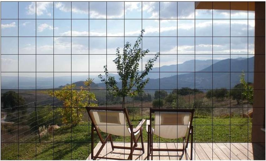
2       M. Khoroshiltseva et al.

and broken artifacts [9], can be seen as jigsaw puzzles with missing information
(boundaries or entire pieces). This task has been only partially explored in the
last year due to its complexity [4,18].
    In this paper, we propose to extend [13] for the case where the borders of the
patches are ruined. To simulate the erosion in the puzzle, we create gaps between
pieces removing pixels lying on the borders. The gaps interrupt the color and
the line continuation between patches, making compatibility functions unusable
or highly inaccurate.
    To alleviate this problem, we adopt an image extension technique; the idea
is to extend the patches borders to cover the eroded parts in the picture with
synthetically generated pixels. Image inpainting and extension are broadly stud-
ied in computer vision, and various techniques were proposed [25,26,6,16,2]. We
consider that the image extension model is more suitable for our task, as we
want to extend the images outside the original border rather than filling missing
parts inside of each patch. The GAN-based model for image extension proposed
in [25] shows impressive results, hence we adopt their model for our procedure:
first, we recover the eroded borders of each patch by extending it in all directions
and we compute the pairwise compatibility on repaired patches; then we apply
the solver [13] to reconstruct the image.
    The paper is organized as follow: in section 2 we discuss the state-of-the-art
of puzzle-solving methods; section 3 details our model, sections 3.1, 3.2 discus
the image extension model and the compatibility computation, respectively; in
section 3.3 we recipe our puzzle solver, and finally we discuss the experiments
and present our results in section 4.

2   Related works

In recent years, the image jigsaw problem has been tackled with different com-
putational approaches proposing a variety of solutions. Cho et al. [5] presented
a graphical model based on the patch transform and proposed an algorithm
that minimizes a probability function via loopy belief propagation. Pomeranz
et al. [20] introduced the first fully automatic puzzle solver proposing a greedy
placer and a novel prediction-based dissimilarity. Their approach relies on find-
ing pairs of pieces with a very high probability of being together. Sholomon et
al. [22] proposed a solver based on a genetic algorithm that can solve large puz-
zles. Paikin et al. [17] extended the work in [20] by solving puzzles with unknown
orientations and with missing pieces, introducing new affinity measures. Son et
al. [24] considerably improved solving puzzles with unknown orientation by us-
ing loop constraints. Andalo et al. [1] presented a global formulation for jigsaw
problems, optimizing the affinity between adjacent pieces by numerically solving
a constrained quadratic program. Gallagher et al. [10] represented a puzzle as a
graph, their algorithm considers edges connecting all pieces in all possible geo-
metric combinations and then trims edges by finding a Minimum Spanning Tree.
Brandao et al. [3] extended the work introduced in [10] by modeling the jigsaw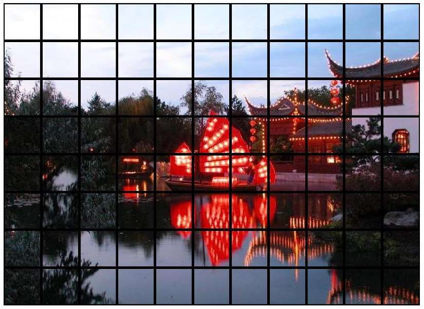
JiGAN: Jigsaw Puzzles with Missing Borders         3

problem as an edge selection problem in a graph, where the nodes represented
the various tile orientations.
     In [13] the puzzle-solving problem is tackled as a problem of finding a consis-
tent labeling that satisfies certain compatibility relations. The problem is solved
using the classical relaxation labeling algorithm coupled with the Sinkhorn-Knop
matrix normalization procedure [23], while adopting the Mahalanobis gradient
compatibility function [10] to calculate the affinity of the parts.
     Only a few papers addressed solving jigsaw puzzles when borders are missing.
Paumard et al. [18] tackled the 3x3 puzzle problem with a probabilistic model; to
emulate the erosion, they randomly cropped a fragment inside each piece; then,
given a central fragment, they used a neural network to predict the relative po-
sitions of the remaining fragments and computed the shortest path in the graph
to reassemble the puzzle. Bridger et al. [4] proposed a method to solve the puzzle
with ruined regions; first, they recovered the missing parts using a GAN-based
model and then reconstructed the image using greedy solver form [17]. Although
the method works nicely, it is computationally intensive since it considers all the
possible combinations of patches pairs and their relations. Ru Li et al. [15] intro-
duce JigsawGAN, a self-supervised GAN-based approach, that combines global
semantic information and edge information of each piece, to solve 3x3 puzzle.
The output of the model is then a permutation matrix of all the pieces.
     Similarly to Bridger et al. [4], this paper tackles the puzzle problem with
ruined regions; however, their work differs from ours in two crucial points: i) [4]
fills in the gaps in the image by applying inpainting algorithm to each pair of
patches for all possible transformations; instead, we recover the damaged borders
of each single patch using image extension algorithm. That is more convenient
from a computational point of view. ii) [4] uses a solver based on naive greedy
placer; instead, we cast the problem as a consistent labeling problem [12], and
solve the puzzle using the relaxation labeling algorithm that enjoys excellent
theoretical properties [19].
     To summarize, the contributions of this paper are three-fold:
 1. This is the first paper proposing a model that exploits generative adversarial
    networks and relaxation labeling processes together
 2. We extended a previous model to handle a more complex task, such as jigsaw
    puzzles with eroded borders
 3. We show the feasibility of our model on a variety of different datasets.

3   Model
In this section, we introduce JiGAN, our GAN-based approach to solving jig-
saw puzzles. Suppose we are given N images, that represent the patches of the
puzzle; the borders of the patches are eroded implying the gaps between parts
in the puzzle. The goal is to reassemble the original image or, saying differently,
assign a position in a 2-dimensional grid assemble plane to each patch of the
puzzle. As in previous works, we assume that the patches are of the same size,
4            M. Khoroshiltseva et al.

    1                           Border Extension       2                                Pairwise Compatibility

                    Boundless                                                     MGC
                      GAN

                     3                                           Final Solution

                                             Relaxation
                                              Labeling
                                               Solver

Fig. 1. Pipeline of the algorithm. ○
                                   1 Given a patch, we extend its borders using Bound-
less GAN [25]. ○2 We exploited the generated borders and compute pairwise compati-
bility between all the patches using Mahalanobis Gradient Compatibility (MGC) [10].
○3 Relaxation Labeling is then used to find a consistent labeling (positioning) of each
piece.

the orientation is known, and the gaps created by eroded borders are of the same
regular size. Our model is illustrated in Figure 1 and is based on three following
key ideas: 1) extending the eroded patches border using a GAN model; 2) com-
puting dissimilarity score for each pair of patches and transforming dissimilarity
scores in the matrix of compatibility coefficients; 3) given the compatibility map,
running the relaxation labeling puzzle solver and reconstructing the image.

3.1        Border Extension
The various methods for compatibility computation, discussed in previous works
[5,20,24,17], are normally based on the color gradient and the continuation of the
edge, and perform well for puzzles without erosion. However, the gaps created
by erosion, will make any of these functions inaccurate and unreliable. For this
reason we first repair the eroded edges by generating the band of new pixels all
around the given patch. To do this we use an image extension technique called
Boundless [25]. The idea is to extrapolate the image of the patch in all directions,
to cover the void created by the erosion. The Boundless is a GAN-based model
tailored to extend the image content along any direction, i.e. to fill the image
content outside the original boundaries. The extended regions are expected to
match the original area on a structural, textual, and semantic level. For our task,
we use the pre-trained model on Places [28] provided by Google3 . The limitation
of the model is that it is trained to extend the image in one direction (right). In
order to extend the images of the puzzle pieces all around, we pass each piece
through the generator four times by rotating it 90°.
    Formally, given the ĩ-th piece of a puzzle, its extended version is denoted by

                                                   i = Φ(ĩ, β, θ)                                               (1)
3
        Pretrained Boundless model from TensowrflowHub
JiGAN: Jigsaw Puzzles with Missing Borders        5

where β is the percentage of image extension, and Φ(...) is the Boundless model
parametrized by θ. Once the damaged borders get repaired, we can use the
reconstructed patches to calculate the patch compatibility.

3.2   Pairwise Compatibility
The compatibility measure quantifies the affinity between pieces and predicts the
likelihood of two patches to be neighbors. We measure the piece affinity by com-
puting the dissimilarity between the abutting boundary pixels of two adjacent
pieces; to this end, we adopt the Mahalanobis Gradient Compatibility (MGC)
developed by Gallagher [10] and further improved by Son et al. [24]. MGC consid-
ers both the color differences across pieces borders and the directional derivative
differences along the borders. Assuming that the two candidate pieces are posi-
tioned such that piece i is placed to the left of piece j, the dissimilarity measure
ΓR (i, j) is defined as:
                                                    0
               ΓR (i, j) = DR (i, j) + DL (j, i) + DR           0
                                                      (i, j) + DL (j, i).       (2)
The first two terms, DR and DL , penalize the changes in the pixel values across
the boundary in the following way:
                        S
                            (ij)     (ij)         (ij)     (ij)
                        X
                                             −1
          DR (i, j) =     (ΛR (s) − ER (s))ViR  (ΛR (s) − ER (s))>              (3)
                        s=1
        (ij)                                                        (ij)
where ER (s) is the expected change across the boundary, ΛR (s) is the pixel
intensity change across the boundary and ViR is a sample covariance calculated
from samples of the border pixels. DR 0
                                        and DL 0
                                                 are calculated by replacing i(u, v)
with the directional derivatives δ(u, v) = i(u, v) − i(u − 1, v).
    Once the pairwise dissimilarity scores are calculated for each pair of pieces
in all possible neighboring relationships (right, up, left, down), we convert them
to normalized compatibility values, as follows:

                                                ΓR (i, j)
                       CR (i, j) = max 1 −                ,0                    (4)
                                              KminR (i)
    where KminR (i) is the K-min value of the dissimilarity between all other
pieces in relation R to piece i. The smaller the value of K, the more sparse
CR (i, j) becomes, leading to a more efficient relaxation labeling process.

3.3   Relaxation Labeling Puzzle Solver
In our formulation, the puzzle pieces are considered as a set of objects and their
possible positions as a set of labels, the puzzle problem is viewed as the problem
of finding consistent labeling that satisfies certain compatibility relations, with
an additional requirement for one-to-one correspondences between the puzzle’s
tiles and their positions. We solve the puzzle using classical relaxation labeling
algorithm [19] that, starting from the uniform probability (barycentre point)
distribution, progressively updates the assignment matrix till it converges to the
consistent labeling, which in our case corresponds to a permutation matrix.
6       M. Khoroshiltseva et al.

Consistent Labeling Problem In this section we recap some basic concepts of
relaxation labeling. Suppose we are given a set of objects B = {b1 , . . . , bn } and a
set of labels Λ = {λ1 , . . . , λm }, the task is to assign a label to each object in B. To
this end two sources of information are available: (1) local measurements, which
capture the characteristic features of each object, (2) contextual information,
quantitatively expressed a matrix of compatibility coefficients R = [rijλµ ]. The
coefficient rijλµ measures the strength of compatibility between the hypotheses
“bi has label λ” and “bj has label µ”.
    The label assignments for object bi is represented by a probability distribu-
tion pi over all possible labels. Formally, pi ∈ ∆m , where where
                                  (                      m
                                                                        )
                                                         X
                      ∆   m
                              =   x∈R   m
                                            | xλ ≥ 0 ∧         xλ = 1                  (5)
                                                         λ=1

    The compatibility model R is considered “contextual” because it naturally
leads to measures of contextual support (i.e., how much the context supports the
assignment of a particular label λ to object bi ) and defined [12] as
                                     X
                               qiλ =     rijλµ pjµ .                         (6)
                                             j,µ

   A process that relaxes a given inconsistent assignment p towards a more
consistent one, will increase piλ when qiλ is high and decrease it when qiλ is
low. The best-known update rule, that guarantees the converge to a consistent
labeling [19] under non-negativity and symmetry conditions on R, is defined by
the following iterative procedure [21,19]:
                                         piλ (t)qiλ (t)
                          piλ (t + 1) = P                       ∀i, λ                  (7)
                                          µ piµ (t)qiµ (t)

    The initial labeling is a starting point of the process and corresponds to a set
of assignments for the entire set of objects. It can be initialized in different ways
depending on whether some prior knowledge exists or not. If prior knowledge is
not available, the object is assigned the same probability for all labels.
    The relaxation algorithm takes as input an initial (imperfect) labeling as-
signment and progressively updates it according to the compatibility model R.
The process continuous until the fixed point is reached, that correspond to a
consistent labeling (when every object chooses his best label).

Relaxation Labeling Algorithm for Puzzle Solving We cast jigsaw puzzle
solving as a consistent labeling problem. The set of objects B represents the
puzzle pieces, the labels Λ are the positions in the reconstruction plane (hence
m = n), and the task is to assign a different position from Λ to each puzzle piece
from B. The P ∈ ∆n×m is a soft assignment matrix (where each row represents a
probability distribution of the positions for a piece and each column represents a
probability distribution of the
                             P pieces for a position),  ∆n×m is the multi-simplex
with ∆ = {pi | piλ ≥ 0 ∧ λ piλ = 1} and ∆ = {pλ | piλ ≥ 0 ∧ i piλ = 1},
       m                                          n
                                                                     P
JiGAN: Jigsaw Puzzles with Missing Borders         7

Fig. 2. JiGAN(blue) vs RL (red) models: average Direct (a) and Perfect (b) accuracy
then increasing the erosion gaps β.

where piλ is the probability of piece
                                    Pi to choose
                                               P position λ. Thus P = piλ is
doubly stochastic matrix such that λ piλ = i piλ = 1.
    The relaxation labeling update rule guarantees that P is a stochastic matrix
(i.e., rows sum to 1) but does not enforce the same constraint for its columns.
Therefore, the optimization process can converge to a labeling that does not
represent a permutation (producing a solution with multiple pieces assigned the
same position and vice versa). To enforce one-to-one correspondence constraints,
we endow the relaxation process with matrix balancing algorithm, adopting
Sinkhorn-Knopp (SK) normalization [23] . SK algorithm transforms a given non-
negative square matrix to its related doubly stochastic version, by alternately
normalizing the rows and columns. SK is incorporated in our algorithm as an
additional balancing step in each iteration.

4   Experiments & Results

Datasets We assessed the performance considering two benchmarks. First, we
test our method on a large dataset of small (synthetic) images. Following Jig-
sawGAN [15] we create our collection of 1600 images randomly picked up from
PACS dataset [14]. Our collection is divided into 4 object categories (elephant,
guitar, person, house), each of which covers 4 image styles (paintings, photos,
cartoons, and sketches). Each of 1600 images is cut into 72x72 pixels size pieces
generating a 9-pieces puzzle (3x3). For the second test, we apply our method to
three datasets [5,20], widely used as performance benchmarks; each contains 20
images of increasing size. We cut the images into equal size pieces, generating
puzzles of 70, 88, and 150 pieces(for the 1st, 2nd, and 3rd data sets respectively).

Accuracy metrics To evaluate the performance of the algorithm we adopt
three accuracy measures, widely used in literature: Direct Comparison metric,
which measures the ratio of pieces placed in the correct position; the Neighbor
Comparison metric that measures the ratio of correctly assigned neighbors in
the solution, and the Perfect Reconstruction metric that is a binary indicator of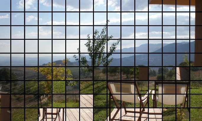
8 M. Khoroshiltseva et al.
0% Erosion gap
7% Erosion gap
14% Erosion gap
Fig. 3. Qualitative results for small puzzles from Pacs dataset (0%, 7%, 14% erosion
of piece size)
0% Erosion gap
7% Erosion gap
14% Erosion gap
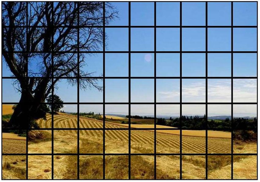
Fig. 4. Qualitative results for big puzzles from Benchmark dataset (0%, 7%, 14% ero-
sion of piece size)
whether all pieces in the puzzle are in the correct position; applied to a dataset,
the Perfect Reconstruction is a ratio of perfectly solved puzzles.
JiGAN: Jigsaw Puzzles with Missing Borders         9

Experiments We performed experiments on the two aforementioned bench-
marks considering the three different metrics and an increasing level of border
erosion, β ∈ {0%, 7%, 14%}. Without erosion (β = 0%) the performance of Ji-
GAN and RL[13] are the same.
    We compare our result to [13] that is our direct competitor, as our model is an
extension of it. Concerning [4], although the idea is similar to ours, their model
involves much more information (all possible pairing and rotation of puzzle’s
pieces), thus a direct comparison would not be fair.
    Experiments with PACS dataset (small puzzles): using the PACs dataset, we
conduct two types of experiments: first, we generate 3x3 puzzles without any gap
between pieces and run the relaxation labeling (RL) solver [13]; second, to simu-
late the erosion of the boards, we generate the puzzles with gaps between pieces
with two different levels of erosion 7% and 14% gaps. We compare two methods:
the RL algorithm without the image extension step, and our JiGAN procedure
that involves the completion of the eroded border.

              Table 1. RL [13] vs. JiGAN(our model). PACS datasets

                    Direct accuracy               Perfect reconstruction
           no gap      7% gap    14% gap      no gap   7% gap      14% gap
            RL      RL JiGAN RL JiGAN          RL RL JiGAN RL JiGAN
   house    0.92    0.57 0.74 0.41 0.60        0.90 0.46 0.64 0.26 0.42
   elephant 0.88    0.51 0.74 0.30 0.54        0.86 0.41 0.64 0.16 0.36
   guitar   0.83    0.42 0.65 0.26 0.48        0.77 0.33 0.49 0.13 0.27
   person   0.90    0.56 0.72 0.40 0.58        0.89 0.51 0.65 0.28 0.43
   mean     0.88    0.50 0.70 0.32 0.53        0.85 0.41 0.60 0.19 0.35

    Table 1 shows the results of puzzle reconstruction in terms of direct compar-
ison accuracy measure and perfect reconstruction ratio. It can be seen that, for
the case without gaps, our solver performs well in all categories. While in the
cases with erosion, the performance of the solver algorithm decreases as the level
of erosion increases. However, the image extension step is beneficial to puzzle
reconstruction concerning the algorithm without extension.
    Nevertheless, the performance of the model degrades with a larger gap and
negatively influences the accuracy of the solver. To further investigate this degra-
dation effect, we perform the experiments by gradually increasing the erosion
gaps and observing the accuracy of the algorithm with and without extension
steps. The plots in figure 2 illustrate the performances of the solver applied to
400 randomly selected puzzles with different levels of erosion. As expected, the
larger the erosion, the less accurate the results.
    Experiments with Benchmark datasets: for further evaluation, we apply our
method to the large puzzles generated from the three benchmark datasets. As
before, we conduct two experiments applying erosion of 7% and 14% of piece size.
Tables 2 shows the results of the RL solver run without reconstruction of the
eroded border and the results of the puzzle solver after the GAN image extension
algorithm is applied. As in the case with small puzzles, the larger erosion gaps,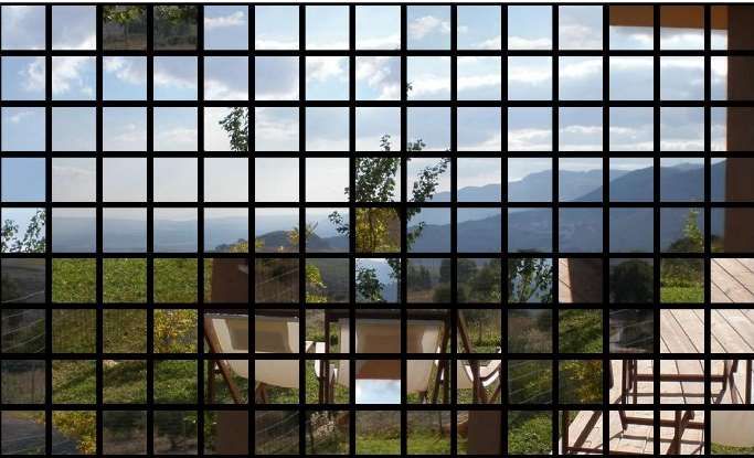
10        M. Khoroshiltseva et al.

             Table 2. RL [13] vs. JiGAN(our model). Benchmark datasets

                        Direct accuracy             Neighbour accuracy
               no gap      7% gap    14% gap   no gap   7% gap    14% gap
                RL       RL JiGAN RL JiGAN      RL RL JiGAN RL JiGAN
     70 pieces  0.97    0.22 0.51 0.11 0.32     0.97 0.46 0.66 0.35 0.45
     88 pieces  0.99    0.23 0.59 0.07 0.31     1.00 0.46 0.65 0.30 0.40
     150 pieces 0.99    0.12 0.38 0.06 0.15     0.99 0.41 0.54 0.28 0.33
     mean       0.98    0.19 0.49 0.08 0.26     0.98 0.45 0.62 0.31 0.39

the lower the accuracy of the puzzle solution. The performance of the GAN
model gradually degrades with the larger area of generated pixels. However,
applying the inpainting algorithm significantly increases the accuracy of puzzle
reconstruction concerning the results of the solver without image extension.
    Figure 4 illustrates some qualitative results of reconstruction results for puz-
zles with different levels of erosion. It can be seen that without erosion we obtain
the perfect reconstruction in most of the cases; for images with 7% of erosion
gap, the overall result is good, however, the images have some errors most of
which are minor and negligible to human eyes. As it can be expected, the results
of reconstruction of images with 14% of erosion are less accurate than those
with 7% of erosion. Though in some examples the misplaced patches make it
difficult the perception the image; in other cases, the reconstruction results are
acceptable for the human eye.

5      Conclusion
In this paper, we extend the method proposed in [13] to handle the challenging
task of solving a puzzle with ruined borders. The previous methods, based on
the compatibility calculated on the color gradient across the edges, effectively
solve the puzzles without gaps, but the performance immediately drops in the
presence of erosion gaps.
    We introduce the idea of repairing damaged patches by involving the GAN
model for image extension. We apply the extension procedure on each patch
separately, thus avoiding expensive inpainting for all combinations in pairs. The
main idea is to regenerate the missing pixels around each patch. Then we calcu-
late the compatibility between the repaired patch and apply the puzzle-solving
algorithm.
    We show that combining of solving algorithm and deep learning model can
be a viable solution to the problem of a puzzle with ruined regions. Our two-step
procedure produces better results compared to the previous method. However,
the quality of the final reconstruction depends on the level of degradation; the
larger the erosion gap, the worse the final result. However, the overall results
with a moderate level of erosion are generally acceptable to human eyes.

Acknowledgements This work has received funding from the European Union’s
Horizon 2020 research and innovation programme under grant agreement No 964854.
JiGAN: Jigsaw Puzzles with Missing Borders 11
References
1. Andaló, F.A., Taubin, G., Goldenstein, S.: PSQP: puzzle solving by quadratic
programming. IEEE TPAMI 39(2), 385–396 (2017)
2. Barnes, C., Shechtman, E., Finkelstein, A., Goldman, D.B.: PatchMatch: A ran-
domized correspondence algorithm for structural image editing. ACM Transactions
on Graphics (Proc. SIGGRAPH) 28(3) (Aug 2009)
3. Brandão, S., Marques, M.: Hot tiles: A heat diffusion based descriptor for automatic
tile panel assembly. In: Hua, G., Jégou, H. (eds.) ECCV Workshops. vol. 9913, pp.
768–782. Springer (2016)
4. Bridger, D., Danon, D., Tal, A.: Solving jigsaw puzzles with eroded boundaries
(2019)
5. Cho, T.S., Avidan, S., Freeman, W.T.: A probabilistic image jigsaw puzzle solver.
In: Proc. CVPR. pp. 183–190 (2010)
6. Clevert, D.A., Unterthiner, T., Hochreiter, S.: Fast and accurate deep network
learning by exponential linear units (elus) (2016)
7. Deever, A., Gallagher, A.: Semi-automatic assembly of real cross-cut shredded
documents. In: Proc. ICIP. pp. 233–236 (2012)
8. Demaine, E.D., Demaine, M.L.: Jigsaw puzzles, edge matching, and polyomino
packing: Connections and complexity. Graphs Comb. 23(Suppl. 1), 195–208 (2007)
9. Derech, N., Tal, A., Shimshoni, I.: Solving archaeological puzzles. CoRR
abs/1812.10553 (2018)
10. Gallagher, A.C.: Jigsaw puzzles with pieces of unknown orientation. In: Proc.
CVPR. pp. 382–389 (2012)
11. Gur, S., Ben-Shahar, O.: From square pieces to brick walls: The next challenge in
solving jigsaw puzzles. In: ICCV. pp. 4029–4037 (2017)
12. Hummel, R.A., Zucker, S.W.: On the foundations of relaxation labeling processes.
IEEE TPAMI 5(3), 267–287 (1983)
13. Khoroshiltseva, M., Vardi, B., Torcinovich, A., Traviglia, A., Ben-Shahar, O.,
Pelillo, M.: Jigsaw puzzle solving as a consistent labeling problem. In: Computer
Analysis of Images and Patterns. pp. 392–402. Springer International Publishing
(2021)
14. Li, D., Yang, Y., Song, Y.Z., Hospedales, T.M.: Deeper, broader and artier domain
generalization. In: Proceedings of the IEEE International Conference on Computer
Vision (ICCV) (Oct 2017)
15. Li, R., Liu, S., Wang, G., Liu, G., Zeng, B.: Jigsawgan: Self-supervised learn-
ing for solving jigsaw puzzles with generative adversarial networks. CoRR
abs/2101.07555 (2021)
16. van den Oord, A., Kalchbrenner, N., Kavukcuoglu, K.: Pixel recurrent neural net-
works (2016)
17. Paikin, G., Tal, A.: Solving multiple square jigsaw puzzles with missing pieces. In:
Proc. CVPR. pp. 4832–4839 (2015)
18. Paumard, M., Picard, D., Tabia, H.: Deepzzle: Solving visual jigsaw puzzles with
deep learning and shortest path optimization. CoRR abs/2005.12548 (2020)
19. Pelillo, M.: The dynamics of nonlinear relaxation labeling processes. J. Math. Imag.
Vis. 7(4), 309–323 (1997)
20. Pomeranz, D., Shemesh, M., Ben-Shahar, O.: A fully automated greedy square
jigsaw puzzle solver. In: Proc. CVPR. pp. 9–16 (2011)
21. Rosenfeld, A., Hummel, R.A., Zucker, S.W.: Scene labeling by relaxation opera-
tions. IEEE Trans. Syst. Man & Cybern. 6, 420–433 (1976)12 M. Khoroshiltseva et al.
22. Sholomon, D., David, O.E., Netanyahu, N.S.: A generalized genetic algorithm-
based solver for very large jigsaw puzzles of complex types. In: Proc. AAAI. pp.
2839–2845 (2014)
23. Sinkhorn, R., Knopp, P.: Concerning nonnegative matrices and doubly stochastic
matrices. Pacific J. Math. 21(2), 343–348 (1967)
24. Son, K., Hays, J., Cooper, D.B.: Solving square jigsaw puzzle by hierarchical loop
constraints. IEEE TPAMI 41(9), 2222–2235 (2018)
25. Teterwak, P., Sarna, A., Krishnan, D., Maschinot, A., Belanger, D., Liu, C., Free-
man, W.T.: Boundless: Generative adversarial networks for image extension (2019)
26. Yu, J., Lin, Z., Yang, J., Shen, X., Lu, X., Huang, T.: Free-form image inpainting
with gated convolution (2019)
27. Zhao, F., He, X., Zhang, Y., Lei, W., Ma, W., Zhang, C., Song, H.: A jigsaw puzzle
inspired algorithm for solving large-scale no-wait flow shop scheduling problems.
Appl. Intell. 50(1), 87–100 (2020)
28. Zhou, Lapedriza, Khosla, Oliva, Torralba: Places: A 10 million image database for
scene recognition 40 (Jun 2018). https://doi.org/10.1109/tpami.2017.2723009You can also read