Robust Object Classification Approach Using Spherical Harmonics
←
→
Page content transcription
If your browser does not render page correctly, please read the page content below
Received January 27, 2022, accepted February 7, 2022, date of publication February 14, 2022, date of current version March 2, 2022.
Digital Object Identifier 10.1109/ACCESS.2022.3151350

Robust Object Classification Approach Using
Spherical Harmonics
AYMAN MUKHAIMAR 1 , (Member, IEEE), RUWAN TENNAKOON                                                          2,   CHOW YIN LAI              3,

REZA HOSEINNEZHAD 1 , AND ALIREZA BAB-HADIASHAR 1
1 Schoolof Engineering, RMIT University, Melbourne, VIC 3000, Australia
2 Schoolof Science, RMIT University, Melbourne, VIC 3000, Australia
3 Department of Electronic and Electrical Engineering, University College London, London WC1E 6BT, U.K.

Corresponding author: Alireza Bab-Hadiashar (alireza.bab-hadiashar@rmit.edu.au)

  ABSTRACT Point clouds produced by either 3D scanners or multi-view images are often imperfect
  and contain noise or outliers. This paper presents an end-to-end robust spherical harmonics approach to
  classifying 3D objects. The proposed framework first uses the voxel grid of concentric spheres to learn
  features over the unit ball. We then limit the spherical harmonics order level to suppress the effect of
  noise and outliers. In addition, the entire classification operation is performed in the Fourier domain. As a
  result, our proposed model learned features that are less sensitive to data perturbations and corruptions.
  We tested our proposed model against several types of data perturbations and corruptions, such as noise and
  outliers. Our results show that the proposed model has fewer parameters, competes with state-of-art networks
  in terms of robustness to data inaccuracies, and is faster than other robust methods. Our implementation code
  is also publicly available at https://github.com/AymanMukh/R-SCNN

  INDEX TERMS Object recognition, point cloud classification, spherical harmonics, robust classification.

I. INTRODUCTION                                                                                 harmonics is a representation that have attracted significant
Objects detection and classification is a crucial part of                                       interest in a wide range of applications including matching
many robotic manipulation applications [1]. For example,                                        and retrieval [13], [14], lighting [15], and surface comple-
autonomous cars or robots can better interact with the sur-                                     tion [16]. They attain several favourable characteristics for
rounding environment if they accurately recognize objects.                                      working with 3D space, such as their basis are defined on the
Due to the existence of compact, low-cost 3D scanners such                                      surface of the sphere (volumetric) and are rotation equivari-
as Microsoft Kinect and Intel RealSense, 3D object measure-                                     ant. In addition, they have shown to provide compact shape
ments are readily available. These scanners generate point                                      descriptors compared to other types of descriptors [13], [17].
clouds either using Light Detection and Ranging (LIDAR)                                            The use of CNNs with spherical harmonics has had major
or using stereo matching. The generated point clouds of                                         success in several recent papers for shape classification [9],
these scanners are often noisy and contain outliers, which                                      [10], [12], retrieval [10] and alignment [10]. Unlike con-
significantly deteriorates the accuracy of existing object clas-                                ventional approaches that use CNNs in regular Euclidean
sification methods.                                                                             domains, spherical harmonics CNNs (SCNNs) apply con-
   The recent success and popularity of Convolutions Neu-                                       volutions in SO(3) Fourier space, learning features that are
ral Networks (CNN) for many computer vision applications                                        SO(3)–equivariant. Frameworks that use spherical harmonics
have inspired researchers to use them for 3D model clas-                                        CNNs can be divided into two groups: Point-based SCNN
sification as well [2]–[4]. To exploit the potential of deep                                    that extract features based on point maps or pairwise rela-
networks for this application, different representations of 3D                                  tions [11], [12] and the other group that uses spherical har-
data have been proposed, including kd-tree [5], dynamic                                         monics convolution on images casted on the sphere [9], [10].
graphs [6], Random Sample Consensus (RANSAC) [7], [8],                                          Interestingly, spherical CNNs have shown to have fewer
and most recently, spherical harmonics [9]–[12]. Spherical                                      parameters [9] and faster training due to the reduction in the
                                                                                                dimensionality of the spherical harmonics shape descriptors,
   The associate editor coordinating the review of this manuscript and                          which make them a suitable candidate for low-cost robots
approving it for publication was Haiyong Zheng              .                                   with limited computational power.
                                           This work is licensed under a Creative Commons Attribution-NonCommercial-NoDerivatives 4.0 License.
VOLUME 10, 2022                                        For more information, see https://creativecommons.org/licenses/by-nc-nd/4.0/                     21541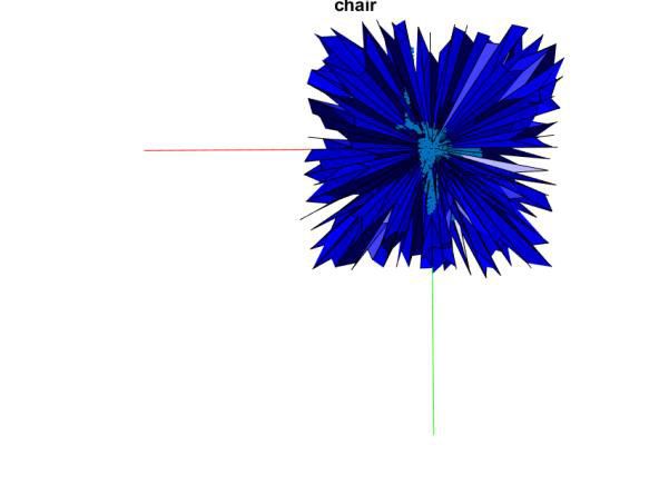
A. Mukhaimar et al.: Robust Object Classification Approach Using Spherical Harmonics
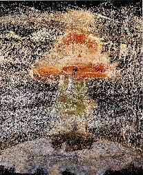
FIGURE 1. a: A 3D model of a scarecrow, b: the point cloud of the scarecrow generated using a
multiview image pipline, data were taken from [18]. c: Point cloud of a scene captured by Intel
RealSense scanner, and d: side of view of the chair captured in c.
Point clouds produced by either 3D scanners or multi-view
images are often imperfect and contain noise and/or outliers.
Several factors lead to those measurements inaccuracies in
the point clouds such as adverse weather conditions, e.g.
fog [19]–[21] and rain [22], [23], objects reflective sur-
face, the scanner itself [24]–[26], or by some pipelines that
construct 3D objects from multi-view images [18], [27],
[28]. Examples of those data inaccuracies can be seen in
Figure 1. The first image shows a scarecrow that was used
for image-based 3D reconstruction. The second image shows
the generated point cloud of the scarecrow using a 3D recon- FIGURE 2. a: Sampling of a line using concentric spheres. The same line
struction algorithm [18], [29]. As seen in Figure 1-b, the is corrupted with outliers in the second row. b: The third concentric
generated point cloud has a high number of outliers surround- sphere corresponding spherical function f (ϕ, θ). c: The same spherical
function f (ϕ, θ) that is shown in b is plotted in the spherical coordinates.
ing the object. The third image shows a scene containing a
chair that was captured by Intel RealSense laser 3D scanner. Unlike previous approaches, our proposed framework per-
The surface of the chair is noisy and surround by outliers, forms the classification in the Fourier domain, where it’s
as seen in the last image. These data inaccuracies make point easier to determine similarities between noisy 3D objects.
cloud classification challenging. As such, the development Moreover, unlike previous approaches [2], [4], [30], the
of robust classification frameworks that can deal with such applied spherical convolution operation is simply multiply-
inaccuracies is needed for autonomous systems and robot ing the filter kernels by the spherical harmonic coefficients,
object interactions. hence, the convolution operation does not disrupt the input
This paper presents a spherical harmonics approach that signal through the use of a pooling operation or grid altering.
is robust to the uncertainty in point clouds data. The pro- We show that the output features produced by the convolution
posed approach is computationally efficient as it requires no operation are highly robust.
pre-processing or filtering of outliers and noise. Instead, our Our experiments show that the use of concentric spheres
entire robust classification operation is performed in an end- with density occupancy grids provides high robustness to
to-end manner. To present our approach, we first discuss the outliers and other types of data inaccuracies. To demonstrate
spherical harmonics descriptors and the common sampling the robustness of the proposed sampling along with the use
strategies used in the literature. We then show that using of spherical harmonic transform, we present a simple case
concentric spheres with density occupancy grids provides the in Figure 2 of a line plotted in 3D. The line was corrupted
highest robustness against data inaccuracies. We also propose with outliers as shown in the second row of the figure in a.
using the magnitude of each specific spherical component Figure 2-b shows the spherical function f (ϕ, θ) of the third
for shape classification, and we show that it produces better concentric sphere, where the distance from the origin (f )
robustness than using the combined magnitudes of different represents the number of points corresponding to each theta
components at each order. In particular, we show that a sim- and phi (plots are in Cartesian for visualization). We plot the
ple classifier (i.e. fully connected neural network) with the same figure in spherical coordinates in Figure 2-c. The max-
previously mentioned spherical harmonics descriptors and imum value of f is one as we are using a density occupancy
sampling strategy is robust to high levels of data inaccura- grid (we divide by max). With the use of density occupancy
cies. Using the above knowledge and the inspiration from grid, outliers appear as small peaks, while inliers have higher
the recent success of spherical CNNs approaches [9], [10], peaks, as can be seen in Figure 2-c. This representation
we propose a light spherical convolutional neural network makes outliers appear as small noise, where noise in Fourier
framework (called RSCNN) that is able to deal with differ- transform (spherical harmonic transform) appears at high
ent types of uncertainty inherent in three-dimensional data frequencies, and our experiments show that by using low
measurement. frequencies, we avoid storing noise in our shape descriptors.
21542 VOLUME 10, 2022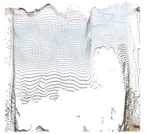
A. Mukhaimar et al.: Robust Object Classification Approach Using Spherical Harmonics

   Our key contributions in this paper are as follows:                                Both of these descriptor vectors have been used for clas-
   • We propose a CNN framework that is significantly more                         sification of shapes [13], [14]. However, only the second
     robust than existing approaches to point cloud inaccura-                      descriptor is rotation equavareint while the first one carries
     cies generated by commercial scanners.                                        more shape information. We have investigated the use of both
   • The proposed approach requires no pre-processing steps                        descriptors for shape classification and the result is provided
     to filter outliers or noise, but instead, the entire robust                   in section III.
     classification operation is performed in an end-to-end
     manner.                                                                       2) SPHERICAL CONVOLUTION
   • The proposed approach uses compact shape descriptors                          If we have a function f with its Fourier coefficients fˆ found
     (spherical harmonics) that reduce the size of our model,                      from Equation (3), and another function or kernel h with
     making it is suitable for low-cost robots with limited                        its Fourier coefficients ĥ, then the convolution operation in
     computational power. We demonstrate the efficiency and                        spherical harmonic domain is equal to the multiplication of
     accuracy of our method on shape classification with                           both functions Fourier coefficients as shown below [31]:
     the presence of several types of data inaccuracies, and                                                       r
                                                                                                                       4π ˆ m 0
     we show that our framework outperforms all previous                                                      m
                                                                                                       (f ∗ h)l =            f ĥ .            (6)
     approaches.                                                                                                     2l + 1 l l
                                                                                      Here, the convolution at degree l and order m is obtained
II. METHODOLOGY                                                                    by multiplying of the coefficient fˆlm with the zonal filter
A. PRELIMINARIES                                                                   kernel ĥ0l . The inverse transform is also achieved by summing
In this section, we review the theory of spherical harmon-                         overall l values:
ics along with their associated descriptors that are used for                                                  X∞ X
classification tasks. In addition, we review the theory of                                    (f ∗ h)(θ, ϕ) =                  l Yl (θ, ϕ).
                                                                                                                        (f ∗ h)m   m
                                                                                                                                               (7)
convolution operations applied to spherical harmonics.                                                      l=0 |m|≤l

1) SPHERICAL HARMONICS                                                             B. RELATED WORK
Spherical harmonics are a complete set of orthonormal basis                        Spherical harmonics have been used for 3D shape
functions, similar to the sines and cosines in the Fourier                         classification for many years [13], [14]. Early classification
series, that are defined on the surface of unit sphere S2 as:                      frameworks used spherical harmonic coefficients as shape
                     s                                                             descriptors [13]. Later, with the use of spherical convolutions,
                       (2l + 1)(l − m)! m                                          classifier networks were empowered to learn descriptive
        Yl (θ, ϕ) =
          m
                                        Pl (cos θ)eimϕ      (1)                    features of objects. We study both approaches in terms of
                          4π(l + m)!
                                                                                   their performance under data inaccuracies.
where Plm (x) is the associated Legendre polynomial, l is the                         The spherical CNNs proposed in [9], [10], for spherical
degree of the frequency and m is the order of every frequency                      signals defined on the surface of a sphere, addresses the rota-
(l ≥ 0, |m| ≤ l). θ ∈ [0, π], ϕ ∈ [0, 2π] denote the                               tion equavarience using convolutions on the set of the 3D
latitude and longitude, respectively. Any spherical function                       rotation group (SO3) and S2 rotation group. In [9], the
f (θ, ϕ) defined on unit sphere S2 can be estimated by the                         spherical input signal is convolved with S2 convolution to
linear combination of these basis functions:                                       produce feature maps on SO3, followed by an SO3 con-
                                X ł
                                ∞ X                                                volution. While zonal filters are used in the spherical con-
                  f (θ, ϕ) =                  fˆlm Ylm (θ, ϕ)                (2)   volutions in [10]. Steerable filters [32]–[34] were used to
                                l=0 m=−l                                           achieve rotation equivariance. The filters use translational
where fˆlm denotes the Fourier coefficient found from:                             weight sharing over filter orientations. The sharing led to a
                 Z π Z 2π                                                          better generalization of image translations and rotations. The
                                     m                                             network filters were restricted to the form of complex circular
     ˆf (l, m) =          f (θ, ϕ)Ȳl (θ, ϕ) sin ϕdϕdθ                       (3)
                      0     0                                                      harmonics [32], or complex valued steerable kernels [33].
                                                                                   Sphnet [12] is designed to apply spherical convolution on
where Ȳ denotes the complex conjugate. The following
                                                                                   volumetric functions [35] generated using extension opera-
descriptors implies that any spherical function can be
                                                                                   tors applied on point cloud data. Unlike previous approaches,
described in terms of the amount of energy |fˆ | it contains at
                                                                                   spherical convolution is applied on point clouds instead of a
every frequency:
                                                                                   spherical voxel grid, resulting in a better rotation equivari-
               D1 = (|fˆ0,0 |, |fˆ1,0 |, |fˆ1,1 |, . . . |fˆlm |),           (4)   ant. In Deepsphere [11], spherical CNNs are used on graph
                                                                                   represented shapes. The shapes are projected onto the sphere
or the amount of energy it contains at every degree:
                                                              v                    using HEALPix sampling, in which the relations between
                                                              u ı
                                                              uX 2                 the pixels of the sphere build the graph. The graph is then
  D2 = (|fˆ0 |, |fˆ1 |, |fˆ2 |, . . . |fˆl |), where |fˆi | = t   fˆ    im   (5)   represented by the Laplacian equation, which is solved using
                                                                 m=−i              spherical CNNs. Ramasinghe et al. [36] investigated the use

VOLUME 10, 2022                                                                                                                              21543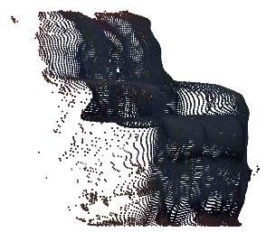
A. Mukhaimar et al.: Robust Object Classification Approach Using Spherical Harmonics

of radial component in spherical convolutions instead of              III. OUR PROPOSED APPROACH
using spherical convolutions on the sphere surface. They              Unlike previous spherical harmonics approaches, our pro-
proposed a volumetric convolution operation that was derived          posed framework, shown in Figure 3, combines the following
from Zernike polynomials. Their results show that the use             three key contributions: the use of concentric spheres, the
of volumetric convolution provides better performance by              direct use of the magnitudes of spherical harmonics coef-
capturing depth features inside the unit ball. Spherical signals      ficients to classify objects, and limiting the spherical har-
have also been used in conjunction with conventional CNNs             monics order level to mitigate the effect of noise/outliers
by [37]–[39] to achieve better rotational equivariance than           to achieve robust classification. To describe our approach,
signals on euclidean space. You et al. [40] used concentric-          we first introduce the problem, then we go through each step
ity to sample 3D models with a sampling strategy that has             of the proposed solution and explain the overall framework.
better robustness to rotations. While previous approaches
used spherical harmonics to build rotation equivariant neural
                                                                      A. PROBLEM STATEMENT
networks, our focus is on building a robust spherical har-
                                                                      Point clouds of 3D models produced by either 3D scanners or
monics structure. As such, our choice of representation is not
                                                                      3D reconstruction algorithms are often imperfect and contain
restricted to spherical harmonics descriptors that are rotation
                                                                      outliers. To test the robustness of previous methods on such
equivariant.
                                                                      scenarios, we recorded 56 scenes, by the Intel RealSense
   In terms of recent deep learning approaches for 3D shape
                                                                      scanner, containing the following common objects: chairs,
classification, 3D CNNs have been used with voxel-based
                                                                      tables, cabinets, sofas, and desks. The recorded objects cat-
3D models [3], [41]–[43] using several occupancy grids [41].
                                                                      egories were chosen from the ScanObjectNN [55] dataset so
Such a representation has shown to be robust to data inac-
                                                                      that we can train methods on the ScanObjectNN training data,
curacies [43] while some implementations (e.g. [44]) have
                                                                      while we test them on our captured data. The ScanObjectNN
achieved very high classification accuracy for clean objects
                                                                      contains real-scene 2.5D objects similar to our scans. How-
(using ModelNet40). Another approach is to use 2D CNN on
                                                                      ever, our recorded objects have higher levels of noise due
images of the 3D mesh/CAD objects rendered from different
                                                                      to the used scanner type and scanning range. Our recorded
orientations [4], [45], [46]. The rendered images are usually
                                                                      objects have noise and outliers with different levels. Exam-
fed into separate 2D CNN layers; a pooling layer follows
                                                                      ples of those objects can be seen in Figure 4. Moreover,
these layers to aggregate their information. These methods
                                                                      to study the effect of each type of inaccuracies on machine
take advantage of existing pertained models to achieve high
                                                                      learning models, we build comprehensive datasets by arti-
classification accuracy. When testing MVCNN [4], the clas-
                                                                      ficially adding noise, outliers, missing points, or a mixture
sification accuracy was heavily affected by data inaccura-
                                                                      of two types. We simulated those data inaccuracies, similar
cies, especially outliers. Another approach uses unsorted
                                                                      to previous studies [2], [6], [7], [30], [56], by adding uni-
and unprocessed point clouds directly as an input to the
                                                                      formly distributed points in the object area (outliers), adding
network layers [2], [6], [30], [47]. These approaches use
                                                                      Gaussian noise to the point clouds, or randomly eliminating
a max-pooling layer that was tested to be robust to point
                                                                      points from objects point clouds (missing points). We used
dropout and noise [48]. However, when tested with out-
                                                                      Gaussian noise as we found out that distributions of measured
liers, their performance was significantly affected. Another
                                                                      noise of 3D scanners are somewhat Gaussian-like as shown in
approach is to build upon relations between points [5]; for
                                                                      Figure 4-e. The standard deviation of the recorded noise was
such methods, the existence of outliers completely changes
                                                                      more than 0.1 in some cases. We measured noise by scanning
the distance graph and causes such an approach to fail.
                                                                      a flat surface, fitting a plane to the point cloud of the surface,
   In terms of robust classification frameworks that exist in
                                                                      and finally recording the points to plane distance distribution.
the literature, Pl-net3D [7] decompose shapes into planar
                                                                      Besides using uniformly distributed outliers, we also test the
segments and classify objects based on the segments informa-
                                                                      robustness of recent methods on clustered outliers. Random
tion. DDN [49] proposes an end-to-end learnable layer that
                                                                      point dropout simulates a case where the scanning density
enables optimization techniques to be implemented in con-
                                                                      varies, i.e., objects are further from the scanner or using a
ventional deep learning frameworks. An m-estimators based
                                                                      scanner with lower scanning density. Examples of those data
robust pooling was proposed instead of max pooling used in
                                                                      perturbations and corruptions can be seen in Figure 5.
conventional CNNs. Our approach shows better robustness to
data argumentation while it involves less computation.
   Although we focus in this paper on single object clas-             B. SAMPLING ON CONCENTRIC SPHERES
sification approaches, some applications require instance             The first step in using the spherical harmonics for modeling
segmentation methods such as [2], [30], [50], [51].                   an object is to sample the input signal, which is referred to
Nevertheless, it is possible to achieve scene segmen-                 as f (ϕ, θ) in Equation (3). Two types of sampling are used
tation with single object classification methods using                in literature [13]: Sampling over the concentric spheres, and
sliding box-based techniques [52], segmentation meth-                 sampling over the sphere surface (image casting). For the
ods such as [53], [54], or utilizing a region proposal                first case, we generate a spherical voxel grid that consists
network [3].                                                          of c concentric spheres with n × n grid resolution for each

21544                                                                                                                             VOLUME 10, 2022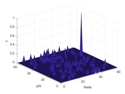
A. Mukhaimar et al.: Robust Object Classification Approach Using Spherical Harmonics

FIGURE 3. The proposed spherical CNN framework: I: We sample the shape with c concentric spheres and n × n grid resolution (section III-B). II: We
apply Fourier transform (FT) on the spherical signal (section II-A1 and section III-C). We get the basis coefficients up to degree l for every concentric
sphere (the first graph in section III of the figure). III: We apply the spherical convolution operation (the second graph in section III of the figure) on the
basis coefficients, where k is the number of filters (section III-D). We then feed the spherical convolution output to a fully connected layer (FC) and a
classification layer (Cl) (section III-E).

concentric sphere. The generated spherical voxel grid allows                       using concentric spheres should provide better robustness to
sampling over the unit ball (S3), with each voxel being rep-                       outliers.
resented by (r, θ, ϕ) where (r = {i − 1, i}, i → 0 : c.
θ, ϕ = {j − 1, j}, j ∗ 2π/n, n → 1 : n). We distribute                             C. CLASSIFICATION IN FREQUENCY DOMAIN
the given 3D shape over the grid, and we keep a record                             Initial spherical harmonics [13], [14] or Fourier [57], [58]
of the number of points inside each voxel and produce a                            based classifiers used the magnitudes of the coefficients
density occupancy grid. The use of such occupancy grid                             to identify similarities between images. Those magnitudes
is expected to provide reliable estimates in the presence of                       were used because they are rotation invariant [13], have
outliers. We compare occupancy grids in the next section.                          low dimensions and importantly they are useful for building
To show the effect of noise and outliers on both sampling                          robust classification techniques [57], [58]. The noise miti-
strategies, we considered a case study shown in Figures 6                          gation property was achieved by discarding the coefficients
and 7. Figure 6 shows sampling over sphere surface for a                           that are greatly affected by noise. For instance, in [58], only
chair shown in column (a), with its corresponding spherical                        frequencies with high magnitudes were used, while in [57],
function f (ϕ, θ) shown in (b), while the generated shape after                    only low-frequency components were used.
applying inverse transform (Equation 2) is shown in (c), and                          Several papers investigated the effect of noise on the
the reconstruction error between b and c is shown in (d).                          Fourier coefficients [58]–[60]. In [58], the authors showed
The first row shows the original shape, while the second                           that for a given image that is perturbed with zero-mean nor-
row shows the shape corrupted with outliers, and finally, the                      mally distributed noise, its corresponding Fourier coefficients
third row shows the shape perturbed with noise. We used a                          have the form:
degree number of l = 10 in those figures. As can be seen
from the second row, outliers heavily affected the generated                                          E[|ĝ(n)|2 ] = |fˆ (n)|2 + |M |σ 2                    (8)
function f (ϕ, θ) shown in b, which affected the reconstructed
shape in c. In contrast, the noise didn’t substantially affect                     where fˆ (n) is the n-th Fourier coefficient of the original
the constructed object when comparing images in c for the                          image, E[x] is the expected value of x, ĝ(n) is the n-th Fourier
first and third rows. Noise in Fourier transform appears at                        coefficient for the noisy image, |M | is the total number of pix-
high frequencies [57], while using low frequencies, such as                        els in the image, and σ is the standard deviation of the additive
here, only captures low details about the object surfaces.                         noise component. According to Equation 8, a particular coef-
Similarly, Figure 7 shows the sampling on concentric spheres                       ficient is a useful feature for a classifier only if |fˆ (n)|2 is much
for the same object, we only show the cases of clean and                           greater than |M |σ 2 , or if the difference between |ĝ(n)|2 and
outliers corrupted object in the first and the second row,                         |fˆ (n)|2 is very small. Although Equation 8 is derived for
respectively. Figure 7-b shows the function f (ϕ, θ) sampled                       Fourier coefficients, its application for the spherical harmon-
from sphere number 3. As can be seen, outliers appear as                           ics coefficients is straightforward as the spherical harmonics
small noise, which is also canceled out, as can be seen in c due                   are an extension to the Fourier transform. As such, we would
to the use of low frequencies. Thus, based on those results,                       expect fˆ (l, m) to be useful if |fˆ (l, m)|2  |M |σ 2 .

VOLUME 10, 2022                                                                                                                                           21545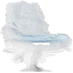
A. Mukhaimar et al.: Robust Object Classification Approach Using Spherical Harmonics
FIGURE 4. a–d: Samples of the recorded objects using Intel RealSense 3D scanner. e: Noise distributing of the
captured signal.
FIGURE 5. (a) The point cloud of a chair taken from the ModelNet40 dataset, (b) the same chair is corrupted with
scattered outliers, (c) the same chair is corrupted with random point dropout, and (d) the same chair is perturbed
with Gaussian noise.
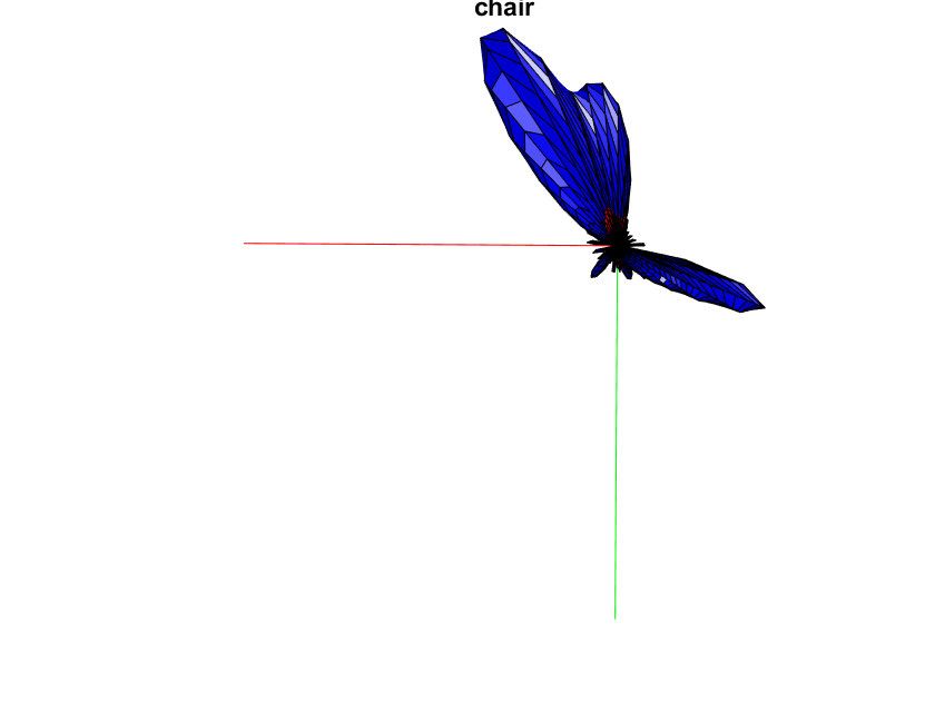
FIGURE 7. a: Sampling of an object (chair) using concentric spheres.
FIGURE 6. Sampling of an object (chair) using image casting, where the b: The third concentric sphere corresponding spherical function f (ϕ, θ).
original object is shown in a, with its corresponding spherical function c: The generated shape after applying Fourier transform (Equation 3)
f (ϕ, θ) shown in b. The generated shape after applying Fourier transform followed by inverse transform (Equation 2). The second row shows the
(Equation 3) followed by inverse transform (Equation 2) is shown in (c), same object corrupted with outliers. All figures are in Cartesian
and the reconstruction error between b and c is shown in (d). The second coordinates.
row shows the same object corrupted with outliers, and the third row
shows the same object perturbed with noise. All figures are in Cartesian
coordinates. reconstructed shapes. Since we limit the use of coefficients
to the orders below 10 (l = 9), outliers are hardly visible in
Based on [57], [58] results, we also limit the order of Figure 8-c.
the spherical harmonics to suppress the effect of noise. Our
experiments show that for a typical object (e.g., the chair in D. IMPLEMENTATION OF SPHERICAL CONVOLUTION
Figure 8) that is perturbed with Gaussian noise, the difference We propose to apply the spherical convolution on 3D models
between the Fourier coefficients of the clean and noisy image that are decomposed into concentric spheres. The use of
increases by increasing the order of the spherical harmonic. concentric spheres generates a uniform spherical voxel grid
As such, limiting spherical harmonics order helps reducing that enables the spherical convolution neural network to learn
the effect of noise. In our classifier, only coefficients up to features over the unit ball (as opposed to only learning over
order 9 were used as further reducing the order will reduce the unit sphere). We use separate convolution operations at
the classification accuracy, as shown in our ablation study each concentric sphere to allow our network to learn features
(see section IV-J). This behaviour is also seen for outliers relevant to that sphere. To achieve the spherical convolution,
as shown in Figure 8. The figure shows that as the degree we use Equation (6) in which the learned kernel is a zonal
level goes higher, outliers start to manifest themselves in the (m = 0) filter h with dimension of l × c, where l is the
21546 VOLUME 10, 2022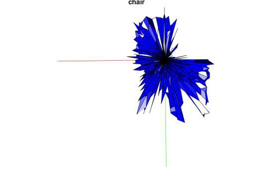
A. Mukhaimar et al.: Robust Object Classification Approach Using Spherical Harmonics

 FIGURE 8. a: Sampling of an object (chair) using concentric spheres. b: The third concentric sphere corresponding spherical function f (ϕ, θ). c: The
 generated shape after applying inverse transform for up to degree 10. d: The generated shape after applying inverse transform for up to degree 50. and
 e: The generated shape after applying inverse transform for up to degree 70.

frequency degree, and c is the number of concentric spheres.                     both clean and perturbed data, as seen from the t-sne results
Similar to [10], we parameterize the kernel filters in the                       (provided in Appendix 1).
spectral domain. No inverse Fourier transform is applied                            Compared to 3D CNNs such as the octnet [43], spherical
after the spherical convolution. Therefore, our convolution                      CNNs are rotation equivariant, which could help in increasing
operation is entirely in the spectral domain, which reduces                      our performance. In addition, the use of spherical convolution
the convolution computation time.                                                has shown to have less trainable parameters, where one layer
   Our results show that applying inverse Fourier trans-                         is enough to achieve good performance [36].
form (IFT) diminishes the robustness to outliers and noise
as the overall accuracy reduces by more than 20 percent.                          E. CLASSIFICATION LAYER
Applying IFT takes us back to the input domain where it’s dif-                   The returned feature map by the convolution operations rep-
ficult to distinguish similarity between two signals compared                    resents the feature vector defined in Equation (4). The map
to the Fourier domain. This can be related to Equation (7),                      is then fed to fully connected and classification layers. The
where for each θ and ϕ, the output signal is calculated by                       feature vector in Equation (5) could be used as well; how-
summing the entire coefficients. Thus, if the coefficients are                   ever, it is less robust to data inaccuracies, as will be shown
already altered by outliers, the output signal error will be                     in the ablation section. Although the feature vector defined
magnified/accumulated due to this summation. A detailed                          in Equation (4) is not rotation invariant, given that we are
discussion on this topic is provided in Appendix 1. Another                      training with rotations, we would expect our network to learn
reason could be due to the reconstruction error shown in                         rotations.
Figure 6-c where IFT contribute to its increase.
   Our experiments show that applying the convolution oper-                       IV. EXPERIMENTS
ation works well with perturbed data and the network has                         We compare our framework with state-of-the-art published
been able to learn better features and be more discerning in                     spherical convolution architectures, point cloud classification
terms of object classification compared to the experiments                       methods, and robust methods. We considered outliers, noise,
shown in Table 7. This is demonstrated by applying t-sne [61]                    and missing points as our types of data inaccuracies in this
to clean and perturbed data, and the results are provided in                     paper since the corruption of point clouds with such inaccu-
Appendix 1. As the application of convolutions on 3D voxel                       racies is common.
grids has shown to be robust to the influence of outliers [48],
we would expect our method to exhibit a high degree of                            A. DATASETS
robustness to outliers as well.                                                  To test the robustness of our approach and other meth-
   Compared to previous approaches, unlike other networks                        ods, we use the benchmarks ModelNet40 [30], [42],
such as PointNet [2] where their max-pooling chooses out-                        ScanObjectNN [55], and shapenet [62] datasets. We also
liers as max, our proposed method does not use pooling or                        build a small dataset that contains 56 scenes of some
grid altering operations. The used convolution operation can                     ScanObjectNN objects captured by Inter RealSense scanner.
be described as follows: Let x ∈ X be our input spherical                        In addition, we used MNIST in the supplementary materials.
coefficient at a given degree li (fˆij , j → 0 : m, m < li ),                    We generate three instances from each of the test sets of
the spherical convolution operation in Equation (6) is simply                    ModelNet40, ScanObjectNN, and shapenet. Each of these
f (x) = k×(x×ĥi ), where ĥi is the kernel value at that degree li              instances is either corrupted with outliers, corrupted with
and k is a constant calculated from the square root term of the                  missing points, or perturbed with noise. We report the classi-
same equation (Equation (6)) followed by the non-linearity                       fication accuracy on each copy individually along with the
operation. This mathematical operation does not alter the                        classification accuracy on the original test set. i.e., for the
input signal and only assists with extracting better features in                 ModelNet40 dataset, which has a test set of 2468 objects,

VOLUME 10, 2022                                                                                                                                   21547
A. Mukhaimar et al.: Robust Object Classification Approach Using Spherical Harmonics

we report the classification accuracy on the original test set,         score around 53%, while PL-Net3D [7] scores 57%. Each
the original test that was perturbed with noise, the original           category in our dataset contains scenes with different noise
test that was corrupted with outliers, and the original test that       levels. As such, methods can identify objects up to a certain
was corrupted with missing points (each test set has the 2,468          noise level. Comparing the results presented in Table 1 show
objects). Figure 5 shows a sample of those perturbations and            that our method can identify objects at higher noise levels
corruptions. For MNIST dataset, we perturb the test set with            compared to other methods.
random noise/outliers at different ratios. The details of these
perturbations and corruptions are explained in the following            TABLE 1. The classification accuracy of some state-of-art methods on our
                                                                        captured scenes.
sections.

B. ARCHITECTURE
The proposed architecture, shown in Figure 3, works with
voxel-based objects. As such, a given 3D shape needs to be
converted to a 3D voxel by dividing the space into a 64*64*7
grid as shown in Figure 3-A. The number of concentric
spheres is chosen to be c=7 (see Figure 13) with a grid
resolution of 64 by 64 for each sphere. The Fourier trans-
form (Equation 3) is applied on each of the seven concentric
spheres to get the spherical harmonics coefficients fˆlm with
l = 9 as the degree of the spherical harmonics. Next, the
spherical convolution (Equation 6) is applied to the spherical          E. ROBUSTNESS TO OUTLIERS
harmonics coefficients. We used one convolution layer (with             In this section, we take the ModelNet40 test dataset and
a size l = 9) having 16 output channels, and used relu after            corrupt it with outliers. Similar to [7], we present two outlier
the convolution operation as our non-linearity. The output of           scenarios generated with different mechanisms. In the first
the convolution layer is then fed into a fully connected layer          scenario, we test our model in the presence of scattered out-
with a size of 1024, followed by a classification layer. The            liers: points uniformly distributed in the unit cube. A sample
spherical convolution kernel ĥ0l applied on each sphere is a           case is shown in Figure 5. In the second scenario, added out-
zonal filter with a size of 1 by 9. The spherical convolution           liers are grouped into clusters of ten or twenty points, which
operation is equivalent to the inner product between a matrix           are uniformly distributed in the unit cube (similar to [65]).
with a size of 9 by 9 that contains the spherical harmonics             The overall number of scattered points for this scenario are
coefficients and a vector of length 9 that represents the con-          fixed to ten or twenty percent as shown in Table 2. Points
volution kernel. We compared different architectures in the             in each cluster are normally distributed with zero mean and
ablation study.                                                         standard deviations of 4% and 6%.
                                                                           In Figure 9, we show the inference time and GPU memory
C. TRAINING                                                             usage for SPHnet, octnet, PL-Net3D and our method. The
We perform data augmentation for training by including ran-             shown inference time include the preprocessing time required
dom rotations around the vertical axis (between 0 − 2π) and             for SPHnet, octnet, and our method to convert the point cloud
small jittering (0.01 Gaussian noise). We take into account             to voxels, and the preprocessing time for PL-Net3D to detect
points normal’s in some scenarios (we mention those scenar-             all the planes in the point cloud using RANSAC. As can be
ios when we report the classification accuracy). The patch              seen from the figure, our method is faster than any other
size is set to 16, the learning rate varies from 0.001 to 0.00004,      compared method, while the iterative RANSAC in PL-Net3D
and the number of epochs is set to 48. We used a TITAN                  takes 100 times longer to detect all the planes in the point
Xp GPU, where only 450Mb of memory was used during                      cloud. The figure also show that our method uses less GPU
training.                                                               memory than other compared methods.
                                                                           Figure 10 and Table 2 show that our model is highly
D. CLASSIFICATION PERFORMANCE ON OUR CAPTURED                           robust to the influences of outlier in both scenarios. The
SCENES                                                                  classification accuracy only drops by 8% percent when half
The classification accuracy of the proposed method and state-           the data are outliers. We get similar robustness to PL-net3D
of-art methods on our datasets are shown in Table 1. The                with the benefit of being much faster (100 times faster), while
dataset contains 56 objects that belong to five categories from         other models robustness drop by significantly higher mar-
the ScanObjectNN dataset (chairs, tables, cabinets, sofas, and          gins. For Spherical-cnn [10], even when we used the median
desks). We train all methods on the ScanObjectNN train-                 aggregation for generating the unit sphere grid (instead of
ing data while we test them on our recorded objects. Our                max aggregation), the network remains sensitive to the influ-
proposed model scores 75% classification accuracy on the                ences of the outliers. Similarly, SpH-net [12] performs poorly
captured scenes, while PointNet [2] and pointCNN [63] score             when there were outliers as these outliers distort the distance
66% classification accuracy. DGCNN [6] and KPConv [64]                  graph.

21548                                                                                                                               VOLUME 10, 2022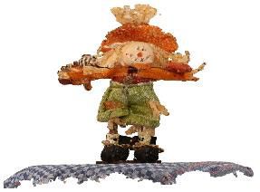
A. Mukhaimar et al.: Robust Object Classification Approach Using Spherical Harmonics

FIGURE 9. GPU memory usage (blue/wide columns) along with the
inference time in seconds (red/thin columns, in log scale) for SPHnet,
octnet, PL-Net3D and our method (RSCNN). The shown times include the
preprocessing time required for SPHnet, octnet, and our method to                FIGURE 11. Classification accuracy versus noise.
convert the point cloud to voxels, and the preprocessing time for
PL-Net3D to detect all the planes in the point cloud.                            TABLE 2. Object classification results on clustered outliers.

                                                                                 model classification accuracy drops by only 2% when half
                                                                                 the points are eliminated, and by 22% when 90% of points
                                                                                 are removed. spherical-cnn classification accuracy drops by
                                                                                 10% when half the points are eliminated and it degrades after
FIGURE 10. Classification accuracy versus outliers.                              that. SPHnet classification accuracy drops by 8% when 60%
                                                                                 of points are eliminated and it degrades after that. Ocntnet
                                                                                 classification accuracy degrades after 50%.
F. ROBUSTNESS TO NOISE
                                                                                    The above results are summarized in Table 3 below. Our
In this section, we use the ModelNet40 dataset and add noise                     proposed model scores 82.2% classification accuracy on
to object points. We simulated the effect of noise in point                      ModelNet40 (MN40) dataset when using points normals,
cloud data by perturbing points with zero mean, normally dis-                    while we achieve 80.5% with points only. Point-based meth-
tributed values with standard deviations ranging from 0.02 to                    ods such as DGCNN [6] and KPConv [64] score around
0.10. A sample case is shown in Figure 5. We used Gaussian                       92% classification accuracy. However, when testing those
noise as we found out that noise in real-scene objects is rela-                  methods on MN40 corrupted with outliers, noise, and missing
tively Gaussian as shown in Figure 4. Figure 11 show that our                    points, our proposed model scores the highest classification
proposed model performance deteriorated the least compared                       performance.
to other models (by around 18%) for relatively large amount
of noise (at 0.10 noise level). This can be related to the use of                 H. CLASSIFICATION ON SHAPENET DATASET
low frequencies, as we mentioned earlier in Figure 6, which
                                                                                 Shapenet dataset contains 51,127 pre-aligned shapes from
cancels the effect of noise. SPHnet was significantly affected
                                                                                 55 categories, which are split into 35,708 for training,
by noise, while spherical-CNN performance was relatively
                                                                                 5,158 shapes for validation and 10,261 shapes for testing.
much better than SPHnet.
                                                                                 Each object contains 2048 points normalized in the unit
                                                                                 cube.1 We tested several methods on this dataset and the
G. ROBUSTNESS TO MISSING POINTS                                                  results are shown in Table 4. PointCNN achieves the highest
In this section, we use the ModelNet40 dataset and randomly
remove points from each object. Figure 12 shows that our                               1 https://github.com/AnTao97/PointCloudDatasets

VOLUME 10, 2022                                                                                                                                  21549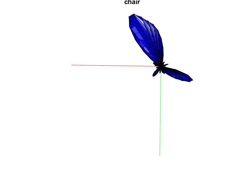
A. Mukhaimar et al.: Robust Object Classification Approach Using Spherical Harmonics

TABLE 3. The classification accuracy on ModelNet40 (MN40) dataset. Noise, Dropout, and OUT are the same dataset when its corrupted with
0.1 Gaussian noise, 90% missing points, and 50% outliers respectively.

                                                                            respectively, while we score the highest classification per-
                                                                            formance when data are corrupted with noise or outliers.
                                                                            KPConv scores the best classification accuracy with a value
                                                                            of 89%, followed by PointCNN with a value of 87%.
                                                                               Comparing the performance of all methods on
                                                                            ScanObjectNN and ModelNet40 datasets shows that all meth-
                                                                            ods classification accuracies (including ours) drop by 4-6%.
                                                                            This could be due to the lower number of training data of
                                                                            ScanObjectNN compared to ModelNet40.
                                                                               PL-Net3D scores 70% classification accuracy with lower
                                                                            robustness to noise, outliers, and missing points. Although
                                                                            KPConv [64] scores the highest classification accuracy on
                                                                            the ScanObjectNN dataset. However it shows low robustness
                                                                            to outliers, noise, and random point dropout along with all
FIGURE 12. Classification accuracy versus missing points.                   other compared methods, except that PointNet shows better
                                                                            robustness to missing points.
classification accuracy with a score of 83%, whereas Point-
Net and DGCNN score around 82%, while KPConv and                            J. ABLATION STUDY
VoxNet score around 81%. Our proposed model scores 77.4%                    We conducted several experiments on the ModelNet40
using points and their normals (75.6% with points only),                    dataset to explore all possible solutions of our method
which is around 3% less than VoxNet and 5% less than the                    and their performance under different data inaccuracies; the
best model.                                                                 results are shown in Table 6. The first row shows the results
   While the performance of the proposed model on clean                     of our proposed model (RSCNN) with 3D Models having
data is slightly lower, it shows significant robustness on the              2000 points and their normals. The second row shows the
corrupted datasets as seen in the table. Pl-Net3D outperforms               results of our proposed model with points only and normal-
our method by 7% on objects corrupted with 50% outliers,                    izing inputs to get a density grid (same results shown in the
however, our model outperforms Pl-Net3D on data corrupted                   previous section). The third row shows the results when train-
with noise and missing points by 12% and 1% respectively.                   ing without normalizing inputs. As can be seen from those
                                                                            results, using density grid provides the best performance. The
I. CLASSIFICATION PERFORMANCE ON ScanObjectNN                               forth row shows the result of our proposed model trained
DATASET                                                                     without points jittering (using points only with normalizing
We corrupt the ScanObjectNN (SC) dataset with 50% outlier,                  inputs).
0.1 Gaussian noise, and 80% missing points. We then report                     We implemented the inverse transform operation after
the classification accuracy of our proposed model along                     applying the convolution in our model. As a result, our model
with some state-of-art models on the corrupted ScanOb-                      performed worse and became less robust to data inaccuracies.
jectNN (SC) in Table 5. Our proposed model scores 76%                       The outputs are presented in the fifth row of Table 6. The
and 76% classification accuracies on the original ScanOb-                   effect of performing Inverse Fourier Transform on the clas-
jectNN (SC) datasets with and without points normal’s                       sification accuracy is discussed in Supplement 1. In the next

21550                                                                                                                                   VOLUME 10, 2022
A. Mukhaimar et al.: Robust Object Classification Approach Using Spherical Harmonics
TABLE 4. The classification accuracy on Shapenet dataset.
TABLE 5. The classification accuracy on ScanObjectNN dataset.
TABLE 6. Classification accuracy versus different network architectures and different data inaccuracies.
TABLE 7. Classification accuracy results for objects perturbed with noise, TABLE 8. Effect of order level on the relative difference
missing points, and outliers. (|ĝ(l , m)|2 − |f̂ (l , m)|2 )/|f̂ (l , m)|2 between coefficients of noisy and clean
image.
step, we evaluated our model with no fully connected layer deviations, uniformly scattered outliers with 50% percentage,
to reduce the number of trainable parameters. However, the and 80% Random point dropout. The results show that the
results, shown in the sixth row, suggest that such an action is used sampling and the density occupancy grid provide a high
detrimental for the overall performance. degree of robustness to outliers. In addition, these results also
We evaluated the robustness of the two descriptors show that the descriptor in Equation (4) D1 provides higher
represented by Equation (4) and Equation (5) for object classification accuracy than using the descriptor in Equa-
classification by feeding each of them to a fully connected tion (5) D2 as the first one carries more shape information.
neural network. The results are shown in Table 7. We tested We tested our method with 5, 7, and 10 concentric spheres.
their robustness against: Gaussian noise with 0.10 standard Each sphere had a 64 by 64 grid. We also tested our method
VOLUME 10, 2022 21551A. Mukhaimar et al.: Robust Object Classification Approach Using Spherical Harmonics
[7] A. Mukhaimar, R. Tennakoon, C. Y. Lai, R. Hoseinnezhad, and
A. Bab-Hadiashar, ‘‘PL-Net3D: Robust 3D object class recognition using
geometric models,’’ IEEE Access, vol. 7, pp. 163757–163766, 2019.
[8] D. Bulatov, D. Stütz, J. Hacker, and M. Weinmann, ‘‘Classification of
airborne 3D point clouds regarding separation of vegetation in complex
environments,’’ Appl. Opt., vol. 60, no. 22, pp. F6–F20, 2021.
[9] T. S. Cohen, M. Geiger, J. Koehler, and M. Welling, ‘‘Spherical CNNs,’’
2018, arXiv:1801.10130.
[10] C. Esteves, C. Allen-Blanchette, A. Makadia, and K. Daniilidis, ‘‘Learning
SO(3) equivariant representations with spherical CNNs,’’ in Proc. Eur.
Conf. Comput. Vis. (ECCV), 2018, pp. 52–68.
FIGURE 13. (a) The Classification accuracy versus number of concentric [11] N. Perraudin, M. Defferrard, T. Kacprzak, and R. Sgier, ‘‘DeepSphere:
spheres. (b) The Classification accuracy versus the spherical harmonics Efficient spherical convolutional neural network with HEALPix sampling
order l . for cosmological applications,’’ Astron. Comput., vol. 27, pp. 130–146,
Apr. 2019.
[12] A. Poulenard, M.-J. Rakotosaona, Y. Ponty, and M. Ovsjanikov, ‘‘Effective
with spherical harmonics orders ranging from 9 to 60. The rotation-invariant point CNN with spherical harmonics kernels,’’ in Proc.
results are shown in Figure 13. Our network performance Int. Conf. 3D Vis. (3DV), Sep. 2019, pp. 47–56.
gradually increases up to using 7 concentric spheres and [13] M. Kazhdan, T. Funkhouser, and S. Rusinkiewicz, ‘‘Rotation invariant
spherical harmonic representation of 3D shape descriptors,’’ in Proc. Symp.
plateaus afterwards. Moreover, increasing the spherical har- Geometry Process., vol. 6, 2003, pp. 156–164.
monics order did not improve the accuracy. [14] D. Wang, S. Sun, X. Chen, and Z. Yu, ‘‘A 3D shape descriptor based on
Table 8 shows that for a typical object (e.g., the chair spherical harmonics through evolutionary optimization,’’ Neurocomputing,
vol. 194, pp. 183–191, Jun. 2016.
in figure 8) that is perturbed with 2% Gaussian noise, the [15] R. Green, ‘‘Spherical harmonic lighting: The gritty details,’’ in Proc. Arch.
difference between the Fourier coefficients of the clean and Game Developers Conf., vol. 56, 2003, p. 4.
noisy image increases by increasing the order of the spherical [16] C. R. Nortje, W. O. C. Ward, B. P. Neuman, and L. Bai, ‘‘Spherical
harmonics for surface parametrisation and remeshing,’’ Math. Problems
harmonic. As such, limiting spherical harmonics order helps Eng., vol. 2015, pp. 1–11, Jan. 2015.
reducing the effect of noise. In our classifier, only coefficients [17] T. Bülow and K. Daniilidis, ‘‘Surface representations using spherical har-
up to order 9 were used as further reducing the order will monics and Gabor wavelets on the sphere,’’ CIS, Minsk, Belarus, Tech.
Rep. MS-CIS-01-37, 2001, p. 92.
reduce the classification accuracy, as shown in Figure 13-b. [18] K. Yücer, A. Sorkine-Hornung, O. Wang, and O. Sorkine-Hornung, ‘‘Effi-
cient 3D object segmentation from densely sampled light fields with
V. CONCLUSION applications to 3D reconstruction,’’ ACM Trans. Graph., vol. 35, no. 3,
pp. 22:1–22:15, Jun. 2016.
Classifying 3D objects is an important task in several robotic [19] M. Bijelic, T. Gruber, and W. Ritter, ‘‘A benchmark for LiDAR sensors
applications. In this paper, we present a robust spherical in fog: Is detection breaking down?’’ in Proc. IEEE Intell. Vehicles Symp.
harmonics model for single object classification. Our model (IV), Jun. 2018, pp. 760–767.
[20] Y. Li, P. Duthon, M. Colomb, and J. Ibanez-Guzman, ‘‘What happens for
uses the voxel grid of concentric spheres to learn features over a ToF LiDAR in fog?’’ IEEE Trans. Intell. Transp. Syst., vol. 22, no. 11,
the unit ball. In addition, we keep the convolution operations pp. 6670–6681, Nov. 2021.
in the Fourier domain without applying the inverse transform [21] K. Qian, S. Zhu, X. Zhang, and L. E. Li, ‘‘Robust multimodal vehicle detec-
tion in foggy weather using complementary LiDAR and radar signals,’’ in
used in previous approaches. As a result, our model is able Proc. IEEE/CVF Conf. Comput. Vis. Pattern Recognit. (CVPR), Jun. 2021,
to learn features that are less sensitive to data inaccuracies. pp. 444–453.
We tested our proposed model against several types of data [22] A. Filgueira, H. González-Jorge, S. Lagüela, L. Díaz-Vilarin̄o, and P. Arias,
‘‘Quantifying the influence of rain in LiDAR performance,’’ Measurement,
inaccuracies, such as noise and outliers. Our results show that vol. 95, pp. 143–148, Jan. 2017.
the proposed model competes with the state-of-art networks [23] C. Goodin, D. Carruth, M. Doude, and C. Hudson, ‘‘Predicting the influ-
in terms of robustness to effects of data inaccuracies with ence of rain on LiDAR in ADAS,’’ Electronics, vol. 8, no. 1, p. 89,
Jan. 2019. [Online]. Available: https://www.mdpi.com/2079-9292/8/1/89
lower computational requirements. [24] X. Cheng, Y. Zhong, Y. Dai, P. Ji, and H. Li, ‘‘Noise-aware unsupervised
deep LiDAR-stereo fusion,’’ in Proc. IEEE/CVF Conf. Comput. Vis. Pat-
REFERENCES tern Recognit. (CVPR), Jun. 2019, pp. 6339–6348.
[25] X. Wang, Z. Pan, and C. Glennie, ‘‘A novel noise filtering model for
[1] U. Weiss and P. Biber, ‘‘Plant detection and mapping for agricultural robots photon-counting laser altimeter data,’’ IEEE Geosci. Remote Sens. Lett.,
using a 3D LiDAR sensor,’’ Robot. Auton. Syst., vol. 59, no. 5, pp. 265–273, vol. 13, no. 7, pp. 947–951, Jul. 2016.
2011. [26] A. H. Incekara, D. Z. Seker, and B. Bayram, ‘‘Qualifying the LiDAR-
[2] R. Q. Charles, H. Su, M. Kaichun, and L. J. Guibas, ‘‘PointNet: Deep learn- derived intensity image as an infrared band in NDWI-based shoreline
ing on point sets for 3D classification and segmentation,’’ in Proc. IEEE extraction,’’ IEEE J. Sel. Topics Appl. Earth Observ. Remote Sens., vol. 11,
Conf. Comput. Vis. Pattern Recognit. (CVPR), Jul. 2017, pp. 652–660. no. 12, pp. 5053–5062, Dec. 2018.
[3] Y. Zhou and O. Tuzel, ‘‘VoxelNet: End-to-end learning for point cloud [27] Z. Song, H. Zhu, Q. Wu, X. Wang, H. Li, and Q. Wang, ‘‘Accurate 3D
based 3D object detection,’’ in Proc. IEEE/CVF Conf. Comput. Vis. Pattern reconstruction from circular light field using CNN-LSTM,’’ in Proc. IEEE
Recognit., Jun. 2018, pp. 4490–4499. Int. Conf. Multimedia Expo (ICME), Jul. 2020, pp. 1–6.
[4] H. Su, S. Maji, E. Kalogerakis, and E. Learned-Miller, ‘‘Multi-view con- [28] D. Dimou and K. Moustakas, Fast 3D Scene Segmentation and Par-
volutional neural networks for 3D shape recognition,’’ in Proc. IEEE Int. tial Object Retrieval Using Local Geometric Surface Features. Berlin,
Conf. Comput. Vis. (ICCV), Dec. 2015, pp. 945–953. Germany: Springer, 2020, pp. 79–98, doi: 10.1007/978-3-662-61364-1_5.
[5] R. Klokov and V. Lempitsky, ‘‘Escape from cells: Deep Kd-networks [29] C. Kim, H. Zimmer, Y. Pritch, A. Sorkine-Hornung, and M. Gross, ‘‘Scene
for the recognition of 3D point cloud models,’’ in Proc. IEEE Int. Conf. reconstruction from high spatio-angular resolution light fields,’’ ACM
Comput. Vis. (ICCV), Oct. 2017, pp. 863–872. Trans. Graph., vol. 32, no. 4, pp. 1–73, Jul. 2013.
[6] Y. Wang, Y. Sun, Z. Liu, S. E. Sarma, M. M. Bronstein, and J. M. Solomon, [30] C. R. Qi, L. Yi, H. Su, and L. J. Guibas, ‘‘PointNet++: Deep hierarchical
‘‘Dynamic graph CNN for learning on point clouds,’’ ACM Trans. Graph., feature learning on point sets in a metric space,’’ in Proc. Adv. Neural Inf.
vol. 38, no. 5, pp. 1–12, 2019. Process. Syst., 2017, pp. 5099–5108.
21552 VOLUME 10, 2022A. Mukhaimar et al.: Robust Object Classification Approach Using Spherical Harmonics
[31] J. R. Driscoll and D. M. J. Healy, ‘‘Computing Fourier transforms and con- [49] S. Gould, R. Hartley, and D. Campbell, ‘‘Deep declarative networks: A new
volutions on the 2-sphere,’’ Adv. Appl. Math., vol. 15, no. 2, pp. 202–250, hope,’’ 2019, arXiv:1909.04866.
1994. [50] W. Wang, R. Yu, Q. Huang, and U. Neumann, ‘‘SGPN: Similarity
[32] D. E. Worrall, S. J. Garbin, D. Turmukhambetov, and G. J. Brostow, group proposal network for 3D point cloud instance segmentation,’’
‘‘Harmonic networks: Deep translation and rotation equivariance,’’ in in Proc. IEEE/CVF Conf. Comput. Vis. Pattern Recognit., Jun. 2018,
Proc. IEEE Conf. Comput. Vis. Pattern Recognit. (CVPR), Jul. 2017, pp. 2569–2578.
pp. 5028–5037. [51] Y. Xu, S. Arai, F. Tokuda, and K. Kosuge, ‘‘A convolutional neural network
[33] M. Weiler, F. A. Hamprecht, and M. Storath, ‘‘Learning steerable filters for point cloud instance segmentation in cluttered scene trained by syn-
for rotation equivariant CNNs,’’ in Proc. IEEE/CVF Conf. Comput. Vis. thetic data without color,’’ IEEE Access, vol. 8, pp. 70262–70269, 2020.
Pattern Recognit., Jun. 2018, pp. 849–858. [52] S. Song and J. Xiao, ‘‘Deep sliding shapes for amodal 3D object detection
[34] M. Weiler, M. Geiger, M. Welling, W. Boomsma, and T. S. Cohen, ‘‘3D in RGB-D images,’’ in Proc. IEEE Conf. Comput. Vis. Pattern Recognit.
steerable CNNs: Learning rotationally equivariant features in volumetric (CVPR), Jun. 2016, pp. 808–816.
data,’’ in Proc. Adv. Neural Inf. Process. Syst., 2018, pp. 10381–10392. [53] B. Douillard, J. Underwood, V. Vlaskine, A. Quadros, and S. Singh,
[35] M. Atzmon, H. Maron, and Y. Lipman, ‘‘Point convolutional neural net- ‘‘A pipeline for the segmentation and classification of 3D point clouds,’’ in
works by extension operators,’’ 2018, arXiv:1803.10091. Experimental Robotics. Berlin, Germany: Springer, 2014, pp. 585–600.
[36] S. Ramasinghe, S. Khan, N. Barnes, and S. Gould, ‘‘Representation learn- [54] A. Teichman, J. Levinson, and S. Thrun, ‘‘Towards 3D object recognition
ing on unit ball with 3D roto-translational equivariance,’’ Int. J. Comput. via classification of arbitrary object tracks,’’ in Proc. IEEE Int. Conf. Robot.
Vis., vol. 128, no. 6, pp. 1–23, 2019. Automat., May 2011, pp. 4034–4041.
[37] W. Boomsma and J. Frellsen, ‘‘Spherical convolutions and their application [55] M. A. Uy, Q.-H. Pham, B.-S. Hua, T. Nguyen, and S.-K. Yeung, ‘‘Revisit-
in molecular modelling,’’ in Proc. Adv. Neural Inf. Process. Syst., 2017, ing point cloud classification: A new benchmark dataset and classification
pp. 3433–3443. model on real-world data,’’ in Proc. IEEE/CVF Int. Conf. Comput. Vis.
[38] Y.-C. Su and K. Grauman, ‘‘Learning spherical convolution for fast fea- (ICCV), Oct. 2019, pp. 1588–1597.
tures from 360 imagery,’’ in Proc. Adv. Neural Inf. Process. Syst., 2017, [56] J. Li, B. M. Chen, and G. H. Lee, ‘‘SO-Net: Self-organizing network
pp. 529–539. for point cloud analysis,’’ in Proc. IEEE/CVF Conf. Comput. Vis. Pattern
[39] B. Coors, A. Paul Condurache, and A. Geiger, ‘‘Spherenet: Learning spher- Recognit., Jun. 2018, pp. 9397–9406.
ical representations for detection and classification in omnidirectional [57] R. Maani, S. Kalra, and Y.-H. Yang, ‘‘Noise robust rotation invariant
images,’’ in Proc. Eur. Conf. Comput. Vis. (ECCV), vol. 2018, pp. 518–533. features for texture classification,’’ Pattern Recognit., vol. 46, no. 8,
[40] Y. You, Y. Lou, Q. Liu, Y.-W. Tai, W. Wang, L. Ma, and C. Lu, ‘‘PRIN: pp. 2103–2116, Aug. 2013.
Pointwise rotation-invariant network,’’ 2018, arXiv:1811.09361. [58] S. Hui and S. H. Żak, ‘‘Discrete Fourier transform based pattern clas-
[41] D. Maturana and S. Scherer, ‘‘VoxNet: A 3D convolutional neural network sifiers,’’ Bull. Polish Acad. Sci., Tech. Sci., vol. 62, no. 1, pp. 15–22,
for real-time object recognition,’’ in Proc. IEEE/RSJ Int. Conf. Intell. Mar. 2014.
Robots Syst. (IROS), Sep. 2015, pp. 922–928. [59] R. Bardenet and A. Hardy, ‘‘Time-frequency transforms of white noises
[42] Z. Wu, S. Song, A. Khosla, F. Yu, L. Zhang, X. Tang, and J. Xiao, ‘‘3D and Gaussian analytic functions,’’ Appl. Comput. Harmon. Anal., vol. 50,
ShapeNets: A deep representation for volumetric shapes,’’ in Proc. IEEE pp. 73–104, Jan. 2021.
Conf. Comput. Vis. Pattern Recognit. (CVPR), Jun. 2015, pp. 1912–1920. [60] J. Huillery, F. Millioz, and N. Martin, ‘‘Gaussian noise time-varying power
[43] G. Riegler, A. O. Ulusoy, and A. Geiger, ‘‘OctNet: Learning deep 3D spectrum estimation with minimal statistics,’’ IEEE Trans. Signal Process.,
representations at high resolutions,’’ in Proc. IEEE Conf. Comput. Vis. vol. 62, no. 22, pp. 5892–5906, Nov. 2014.
Pattern Recognit. (CVPR), Jul. 2017, pp. 3577–3586. [61] L. van der Maaten and G. Hinton, ‘‘Visualizing data using t-SNE,’’ J. Mach.
[44] A. Brock, T. Lim, J. M. Ritchie, and N. Weston, ‘‘Generative and dis- Learn. Res., vol. 9, pp. 2579–2605, Nov. 2008.
criminative voxel modeling with convolutional neural networks,’’ 2016, [62] A. X. Chang, T. Funkhouser, L. Guibas, P. Hanrahan, Q. Huang,
arXiv:1608.04236. Z. Li, S. Savarese, M. Savva, S. Song, H. Su, J. Xiao, L. Yi, and
[45] E. Johns, S. Leutenegger, and A. J. Davison, ‘‘Pairwise decomposition of F. Yu, ‘‘ShapeNet: An information-rich 3D model repository,’’ 2015,
image sequences for active multi-view recognition,’’ in Proc. IEEE Conf. arXiv:1512.03012.
Comput. Vis. Pattern Recognit. (CVPR), Jun. 2016, pp. 3813–3822. [63] Y. Li, R. Bu, M. Sun, W. Wu, X. Di, and B. Chen, ‘‘PointCNN: Convolution
[46] C. Wang, M. Pelillo, and K. Siddiqi, ‘‘Dominant set clustering and pooling on X-transformed points,’’ in Proc. Adv. Neural Inf. Process. Syst., vol. 31,
for multi-view 3D object recognition,’’ 2019, arXiv:1906.01592. 2018, pp. 820–830.
[47] Y. Ben-Shabat, M. Lindenbaum, and A. Fischer, ‘‘3DmFV: Three- [64] H. Thomas, C. R. Qi, J.-E. Deschaud, B. Marcotegui, F. Goulette, and
dimensional point cloud classification in real-time using convolutional L. Guibas, ‘‘KPConv: Flexible and deformable convolution for point
neural networks,’’ IEEE Robot. Autom. Lett., vol. 3, no. 4, pp. 3145–3152, clouds,’’ in Proc. IEEE/CVF Int. Conf. Comput. Vis. (ICCV), Oct. 2019,
Oct. 2018. pp. 6411–6420.
[48] A. Mukhaimar, R. Tennakoon, C. Y. Lai, R. Hoseinnezhad, and [65] X. Ning, F. Li, G. Tian, and Y. Wang, ‘‘An efficient outlier removal method
A. Bab-Hadiashar, ‘‘Comparative analysis of 3D shape recognition in the for scattered point cloud data,’’ PLoS ONE, vol. 13, no. 8, Aug. 2018,
presence of data inaccuracies,’’ in Proc. IEEE Int. Conf. Image Process. Art. no. e0201280.
(ICIP), Sep. 2019, pp. 2471–2475.
VOLUME 10, 2022 21553You can also read