SINGLE TRIAL DECODING OF SCALP EEG UNDER NATURALISTIC STIMULI - bioRxiv
←
→
Page content transcription
If your browser does not render page correctly, please read the page content below
bioRxiv preprint first posted online Nov. 29, 2018; doi: http://dx.doi.org/10.1101/481630. The copyright holder for this preprint
  (which was not peer-reviewed) is the author/funder, who has granted bioRxiv a license to display the preprint in perpetuity.
                                 It is made available under a CC-BY-ND 4.0 International license.

        SINGLE TRIAL DECODING OF SCALP EEG UNDER NATURALISTIC STIMULI

         Greta Tuckute, Sofie Therese Hansen, Nicolai Pedersen, Dea Steenstrup, Lars Kai Hansen

                  Department of Applied Mathematics and Computer Science (DTU Compute)
                    Technical University of Denmark, DK-2800 Kongens Lyngby, Denmark
                                             {grtu, lkai}@dtu.dk

                          ABSTRACT                                             In case of scalp EEG, this research area is still pro-
                                                                           gressing, and relatively few studies document detection of
There is significant current interest in decoding mental states            brain states in regards to semantic categories (often dis-
from electro-encephalography (EEG) recordings. We demon-                   crimination between two high-level categories) [Simanova
strate single trial decoding of naturalistic stimuli based on              et al., 2010, Murphy et al., 2011, Taghizadeh-Sarabi et al.,
scalp EEG acquired with user-friendly, portable, 32 dry elec-              2014, Kaneshiro et al., 2015, Zafar et al., 2017].
trode equipment. We show that Support Vector Machine
                                                                               Due to before-mentioned challenges, previous studies
(SVM) classifiers trained on a relatively small set of de-
                                                                           have been performed in laboratory settings with high-grade
noised (averaged) trials perform at par with classifiers trained
                                                                           EEG acquisition equipment [Simanova et al., 2010, Murphy
on a large set of noisy samples. We propose a novel method
                                                                           et al., 2011, Stewart et al., 2014, Kaneshiro et al., 2015, Za-
for computing sensitivity maps on EEG-based SVM clas-
                                                                           far et al., 2017]. Visual stimuli conditions can often not
sifiers for visualization of the EEG signatures exploited by
                                                                           be described as naturalistic [Simanova et al., 2010, Murphy
SVM classifiers. We apply the NPAIRS framework for es-
                                                                           et al., 2011, Taghizadeh-Sarabi et al., 2014, Stewart et al.,
timation of map uncertainty. We show that effect size plots
                                                                           2014, Kaneshiro et al., 2015] and individual trials are re-
are similar for classifiers trained on small samples of de-
                                                                           peated multiple times [Simanova et al., 2010, Murphy et al.,
noised data and large samples of noisy data. We conclude
                                                                           2011, Stewart et al., 2014, Kaneshiro et al., 2015, Zafar et al.,
that the average category classifier can successfully predict
                                                                           2017] in order to average the event related potential (ERP)
on single-trial subjects, allowing for fast classifier training,
                                                                           response for further classification purposes. Moreover, a
parameter optimization and unbiased performance evaluation.
                                                                           number of participants are typically excluded from analysis
                                                                           due to artifacts and low classification accuracy [Taghizadeh-
                                                                           Sarabi et al., 2014, Zafar et al., 2017].
                     1. INTRODUCTION                                           The motivation for the current study is to overcome the
                                                                           highlighted limitations in EEG-based decoding. Therefore,
Decoding of brain activity aims to reconstruct the perceptual              we acquired EEG data in a typical office setting using a user-
and semantic content of neural processing, based on activity               friendly, portable, wireless EEG Enobio system with 32 dry
measured in one or more brain imaging techniques, such as                  electrodes. Stimuli consisted of naturalistic images from the
electro-encephalography (EEG), magneto-encephalography                     Microsoft Common Objects in Context (MS COCO) image
(MEG) and functional magnetic resonance imaging (fMRI).                    database [Lin et al., 2014], displaying complex everyday
EEG-based decoding of human brain activity has significant                 scenes and non-iconic views of objects from 23 different
potential due to excellent time resolution and a possibility of            semantic categories. All images presented were unique and
real-life acquisition, however, the signal is extremely diverse,           not repeated for the same subject throughout the experiment.
highly individual, sensitive to disturbances, and has a low                We acquired data from 15 healthy participants (5 female).
signal to noise ratio, hence, posing a major challenge for both            We are interested in exploring the limitations of inter-subject
signal processing and machine learning [Nicolas-Alonso and                 generalization, i.e., population models, hence no participants
Gomez-Gil, 2012]. Decoding studies based on fMRI have                      are excluded from analysis. Decoding ability is evaluated in
matured significantly during the last 15 years, see e.g. [Ger-             a between-subjects design, i.e., in a leave-one-subject-out ap-
lach, 2007, Loula et al., 2018]. These studies successfully                proach (as opposed to within-subject classification) to probe
decode human brain activity from naturalistic visual stimuli               generalizability across participants.
and movies [Kay et al., 2008, Prenger et al., 2009, Nishimoto                  The work in the current study is focused on the binary
et al., 2011, Huth et al., 2012, Huth et al., 2016, Güçlü and           classification problem between two classes: brain process-
van Gerven, 2017].                                                         ing of animate and inanimate image stimuli. Kernel methods,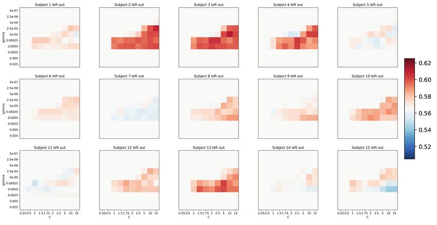
bioRxiv preprint first posted online Nov. 29, 2018; doi: http://dx.doi.org/10.1101/481630. The copyright holder for this preprint
  (which was not peer-reviewed) is the author/funder, who has granted bioRxiv a license to display the preprint in perpetuity.
                                 It is made available under a CC-BY-ND 4.0 International license.

e.g., support vector machines (SVM) are frequently applied                 image, and 3) Minimum 30 images within the category. Fur-
for learning of statistical relations between patterns of brain            thermore, we ensured that all 690 images had a relatively sim-
activation and experimental conditions. In classification of               ilar luminance and contrast to avoid the influence of low-level
EEG, SVMs have shown good performance in many contexts                     image features in the EEG signals. Thus, images within 77%
[Lotte et al., 2007, Murphy et al., 2011, Taghizadeh-Sarabi                of the brightness distribution and 87% of the contrast distri-
et al., 2014, Stewart et al., 2014, Andersen et al., 2017]. SVM            bution were selected. Images that were highly distinct from
allows adoption of a nonlinear kernel function to transform                standard MS COCO images were manually excluded (see Ap-
input data into a high dimensional feature space, where it is              pendix B for exclusion criteria). Stimuli were presented using
possible to linearly separate data. The iterative learning pro-            custom Python scripts built on PsychoPy2 software [Peirce,
cess of the SVM will devise an optimal hyperplane with the                 2009].
maximal margin between each class in the high dimensional
feature space. Thus, the maximum-margin hyperplane will
                                                                           2.3. EEG Data Collection
form the decision boundary for distinguishing different ani-
mate and inanimate data [Saitta, 1995].                                    A user-friendly EEG equipment, Enobio (Neuroelectrics)
    We adopt a novel methodological approach for comput-                   with 32 channels and dry electrodes, was used for data
ing and evaluating SVM classifiers based on two SVM ap-                    acquisition. The EEG was electrically referenced using a
proaches: 1) Single trial training and test classification, and 2)         CMS/DRL ear clip. The system recorded 24-bit EEG data
Training on a meaned response of each of the 23 image cate-                with a sampling rate of 500 Hz, which was transmitted wire-
gories for each subject (corresponding to 23 trials per subject)           lessly using Wifi. LabRecorder was used for recording EEG
and single trial test classification. Furthermore, we open the             signals. Lab Streaming Layer (LSL) was used to connect
black box and visualize which parts of the EEG signature are               PsychoPy2 and LabRecorder for unified measurement of
exploited by the SVM classifiers. In particular, we propose a              time series. The system was implemented on a Lenovo Le-
method for computing sensitivity maps on EEG-based SVM                     gion Y520, and all recordings were performed in a normal
classifiers based on a methodology originally proposed for                 office setting.
fMRI [Rasmussen et al., 2011]. For evaluation of effect sizes
of ERP difference maps and sensitivity maps, we use a modi-
fied version of an NPAIRS resampling scheme [Strother et al.,              2.4. EEG Preprocessing
2002]. Lastly, we investigate how the classifier based on the              Preprocessing of the EEG was done using EEGLAB (sccn.
average EEG category response compares to the single-trial                 ucsd.edu/eeglab). The EEG signal was bandpass filtered to 1-
classifier in terms of prediction accuracy of novel subjects.              25 Hz and downsampled to 100 Hz. Artifact Subspace Recon-
                                                                           struction (ASR) [Mullen et al., 2015] was applied in order to
            2. MATERIALS AND METHODS                                       reduce non-stationary high variance noise signals. Removed
                                                                           channels were interpolated from the remaining channels, and
2.1. Participants                                                          the data was subsequently re-referenced to an average refer-
                                                                           ence. Epochs of 600 ms, 100 ms before and 500 ms after
A total of 15 healthy subjects with normal or corrected-to-
                                                                           stimulus onset, similar to [Kaneshiro et al., 2015], were ex-
normal vision (10 male, 5 female, mean age: 25, age range:
                                                                           tracted for each trial. A sampling drift of 100 ms throughout
21-30), who gave written informed consent prior to the ex-
                                                                           the entire experiment was observed for all subjects and was
periment, were recruited for the study. Participants reported
                                                                           corrected for offline.
no neurological or mental disorders. Non-invasive experi-
ments on healthy subjects are exempt from ethical committee                    Since the signal-to-noise ratio varied across trials and par-
processing by Danish law [Den Nationale Videnskabsetiske                   ticipants, all signals were normalized to z-score values (i.e.,
Komité, 2014]. Among the 15 recordings, no participants                   each trial from each participant was individually transformed
were excluded, as we would like to generalize our results to a             so that it had a mean value of 0 and a standard deviation of 1
broad range of experimental recordings.                                    across time samples and channels).

2.2. Stimuli                                                               2.5. Experimental Design
Stimuli consisted of 690 images from the Microsoft Common                  Participants were shown 23 blocks of trials composed of 30
Objects in Context (MS COCO) dataset [Lin et al., 2014].                   images each. Of the 23 categories, 10 categories contained
Images were selected from 23 semantic categories, with each                animals and the remaining 13 categories contained inanimate
category containing 30 images. All images presented were                   items, such as food or objects. Each block corresponded to
unique and not repeated for the same subject throughout the                an image category (for categories and images used in the ex-
experiment. The initial selection criteria were 1) Image as-               periment, see Supplementary File 1), and the order of cate-
pect ratio of 4:3, 2) Only a single super- and subcategory per             gories and images within the categories was random for each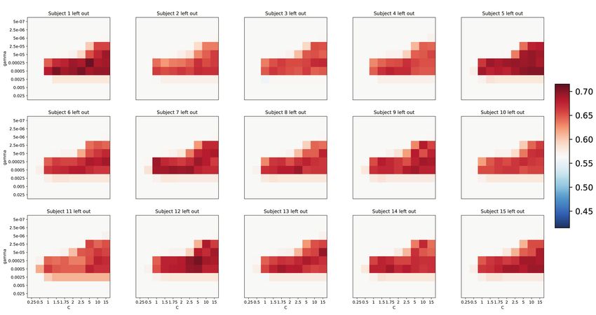
bioRxiv preprint first posted online Nov. 29, 2018; doi: http://dx.doi.org/10.1101/481630. The copyright holder for this preprint
  (which was not peer-reviewed) is the author/funder, who has granted bioRxiv a license to display the preprint in perpetuity.
                                 It is made available under a CC-BY-ND 4.0 International license.

subject. At the beginning of each category, a probe word de-               fier. Both classifiers decode the supercategories, animate ver-
noting the category name was displayed for 5 s followed by                 sus inanimate, and they both classify between subjects. The
30 images from the corresponding category. Each image was                  single-trial classifier is trained on 690 trials for each subject
displayed for 1 s, set against a mid-grey background. Inter-               included in the training set. The average category classifier
stimuli intervals (ISI) of variable length were displayed be-              averages within the 23 categories for each subject, such that
tween each image. The ISI length was randomly sampled ac-                  the classifier is trained on 23 epochs for each subject included
cording to a uniform distribution from a fixed list of ISI values          in the training set, instead of 690 epochs.
between 1.85 s and 2.15 s in 50 ms intervals, ensuring an aver-                 The performance of the single-trial classifier was esti-
age ISI duration of 2 s. To minimize eye movements between                 mated by using 14 participants as the training set, and the
trials, the ISI consisted of a white fixation cross superimposed           remaining participant was used as the test set (SVM param-
on a mid-grey background in the center of the screen.                      eters visualized in Figure S7). Cross-validation was per-
     Subjects viewed images on a computer monitor on a desk                formed on 10 parameter values in ranges c = [0.05; 10] and
with a viewing distance of 57 cm. The size of stimuli was 4                γ = [2.5 × 10⁻⁷ ; 5 × 10⁻³ ], thus cross-validating across 100
x 3 degrees of the visual angle. Duration of the experiment                parameter combinations for each held out subject.
was 39.3 min, which included five 35 s breaks interspersed                      For an debiased estimate of test accuracy, the single-trial
between the 23 blocks. Before the experimental start, partic-              classifier was trained on 13 subjects, with 2 participants held
ipants underwent a familiarization phase with two blocks of                out for validation and test in each iteration. Fifteen classi-
reduced length (103 s).                                                    fiers were trained with different subjects held out in each it-
                                                                           eration. An optimal parameter set of c and γ was estimated
2.6. Support Vector Machines                                               using participants 1-7 as validation subjects (mean parame-
                                                                           ter value), which was used to estimate the test accuracy for
Support vector machines (SVM) were implemented to clas-                    subjects 8-15 and vice versa. Thus, two sets of optimal pa-
sify the EEG data into two classes according to animate and                rameters were found (Figure S9). Cross-validation was per-
inanimate trials. yi ∈ {−1, 1} is the identifier of the category,          formed on 10 parameter values in ranges c = [0.25; 15] and
and an observation is defined to be the EEG response in one                γ = [5 × 10⁻⁷ ; 2.5 × 10⁻² ].
epoch ([−100, 500] ms w.r.t. stimulus onset).                                   The average category level classifier is much faster to
    The SVM classifier is implemented by a nonlinear projec-               train and was built using a basic nested leave-one-subject-
tion of the observations xn into a high-dimensional feature                out cross-validation loop. In the outer loop, one subject was
space F.                                                                   held out for testing while the remaining 14 subjects entered
    Let φ : X → − F be a mapping from the input space X to                 the inner loop. The inner loop was used to estimate the
F. The weight vector w can be expressedPN as a linear com-                 optimum c and γ parameters for the SVM classifier. The
bination of the training points w = n=1 αn φ(xn ) and the                  performance of the model was calculated based on the test
kernel trick is used to express the discriminant function as:              set. Each subject served as test set once. A permutation
                                                                           test was performed to check for significance. For each left
                                     N                                     out test subject, the animacy labels were permuted and com-
                                     X
         y(x; θ) = α> kx + b =             αn k(xn , x) + b        (1)     pared to the predicted labels. This was repeated 1000 times,
                                     n=1                                   and the accuracy scores of the permuted sets were compared
                                                                           against the accuracy score of the non-permuted set. The
    with the model now parametrized by the smaller set of pa-              upper level of performance was estimated by choosing the
rameters θ = {α, b} [Lautrup et al., 1994]. The Radial Basis               parameters based on the test set. Cross-validation was per-
Function (RBF) kernel allows for implementation of a non-                  formed on 10 parameter values in ranges c = [0.25; 15] and
linear decision boundary in the input space. The RBF kernel                γ = [5 × 10⁻⁷ ; 2.5 × 10⁻² ].
kx holds the elements:
                                                                           2.7. Sensitivity mapping
                                                   2
               k(xn , x) = exp (−γ||xn − x|| )                     (2)     To visualize the SVM RBF kernel, the approach proposed by
                                                                           [Rasmussen et al., 2011] was adapted. The sensitivity map is
     where γ is a tunable parameter.                                       computed as the derivative of the RBF kernel, c.f. Eq. (2)
     The SVM algorithm works by identifying a hyperplane in
the feature space that optimally separates the two classes in
the training data. Often it is desirable to allow a few misclas-              ∂α> kx   X                                  2
                                                                                     =   αn 2γ(xn,j − xj ) exp(−γ kxn − xk ) (3)
sifications in order to obtain a better generalization error. This             ∂xj     n
trade-off is controlled by a tunable regularization parameter c.
     Two overall types of SVM classifiers were implemented:                   Pseudo code for computing the sensitivity map across
1) Single-trial classifier, and 2) Average category level classi-          time samples and trials is found in Appendix A.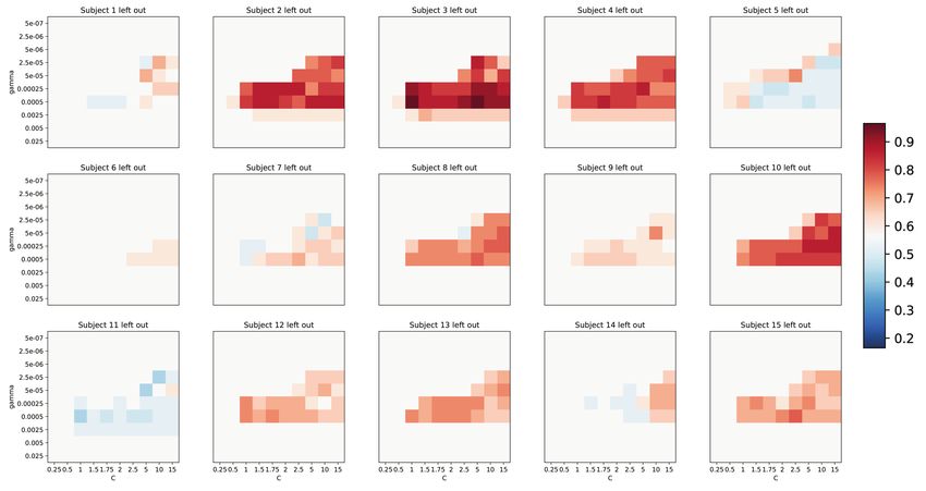
bioRxiv preprint first posted online Nov. 29, 2018; doi: http://dx.doi.org/10.1101/481630. The copyright holder for this preprint
  (which was not peer-reviewed) is the author/funder, who has granted bioRxiv a license to display the preprint in perpetuity.
                                 It is made available under a CC-BY-ND 4.0 International license.

2.8. Effect size evaluation
The NPAIRS (nonparametric prediction, activation, influence,
and reproducibility resampling) framework [Strother et al.,
2002] was implemented to evaluate effect sizes of the SVM
sensitivity map and animate/inanimate ERP differences. The
sensitivity map and the ERP differences based on all subjects
were thus scaled by the average difference of sub-sampled
partitions.
     The scaling was calculated based on S = 100 splits. In
each split, two partitions of the data set were randomly se-
lected without replacement. A partition consisted of 7 sub-
jects, thus achieving two partitions of 7 subjects each (leaving
a single, random subject out in each iteration).
     For evaluation of the ERP difference map, a difference
map was calculated for each partition (M1 and M2 ). Sim-                   Fig. 1. Experimental design of the visual stimuli presentation
ilarly, for evaluation of the sensitivity map, a SVM classi-               paradigm. The time-course of the events is shown. Partic-
fier was trained on each partition, and sensitivity maps were              ipants were shown a probe word before each category, and
computed for both SVM classifiers (corresponding to M1 and                 jittered inter-stimuli intervals consisting of a fixation cross
M2 for the ERP difference map evaluation). The sensitivity                 was added between stimuli presentation. The experiment con-
map for the single-trial SVM classifier was computed based                 sisted of 690 trials in total, 23 categories of 30 trials, ordered
on optimal model parameters, while the sensitivity map of                  randomly (both category- and image-wise) for each subject.
the average category classifier was based on the mean param-
eters as chosen by the validation sets. The maps from the two
partitions were contrasted and squared. Across time samples                to the scalp, an increasing tension of facial muscles or other
(t = 1, . . . , T ) and trials (n = 1, . . . , N ) an average stan-        artifactual currents [Delorme et al., 2007] [Rowan and Tolun-
dard deviation of the average difference between partitions                sky, 2003]. If the data are epoched, the drift may misleadingly
was calculated                                                             appear as a pattern reproducible over trials, a tendency that
                                                                           may be further reinforced by component analysis techniques
                                                                           that emphasize repeatable components [de Cheveigné and
                        S,T,N
                   1     X                         2                       Arzounian, 2018].
           σ2 =                Mi1,t,n − Mi2,t,n )                 (4)          Slow linear drifts can be removed by employing high pass
                  ST N i,t,n=1
                                                                           filters, however more complicated temporal effects are harder
   The full map, Mfull (based on 15 subjects) was then di-                 to remove. We investigated the temporal trend both before
vided by the standard deviation to produce the effect size                 and after Artifact Subspace Reconstruction (ASR) for each
                                                                           subject, see Figures S2 and S3. Generally, the time dependen-
                                                                           cies are reduced by ASR. However, the variance across trials
                           c = Mfull .
                           M                                       (5)
                                σ                                          remains time correlated for subjects 3 and 14 after ASR.

                          3. RESULTS                                       3.2. Event Related Potential analysis

We classify the recorded EEG using SVM RBF models such                     After EEG data preprocessing, we confirmed that our visual
that trials are labeled with the high-level category of their pre-         stimuli presentation elicited a visually evoked potential re-
sented stimuli, i.e., either animate or inanimate. We first re-            sponse. The event related potentials (ERPs) for the trials of
port results using a average category classifier followed by a             animate content and the trials of inanimate content are com-
single-trial SVM classifier, and then apply the average cate-              pared in Figure 2. The grand average ERPs across subjects
gory classifier for prediction of single-trial EEG. Also, we re-           (thick lines) are shown along with the average animate and
port effect sizes of ERP difference maps and sensitivity maps              inanimate ERPs of each subject.
for evaluation of the SVM classifiers.                                         The average animate and inanimate ERPs were most dif-
                                                                           ferent 310 ms after stimuli onset. The average scalp map at
                                                                           this time point can also be seen in Figure 2 for the two super-
3.1. Time Dependency
                                                                           categories as well as the difference between them.
There will naturally be a temporal component in EEG. This                      Inspection of Figure 2 shows that visual stimuli presen-
unwanted non-stationarity of the signal can, for example,                  tation elicited a N100 ERP component at 80-100 ms post-
arise from electrodes gradually loosing or gaining connection              stimulus onset followed by a positive deflection at around
bioRxiv preprint first posted online Nov. 29, 2018; doi: http://dx.doi.org/10.1101/481630. The copyright holder for this preprint
(which was not peer-reviewed) is the author/funder, who has granted bioRxiv a license to display the preprint in perpetuity.
It is made available under a CC-BY-ND 4.0 International license.
Fp1 Fp2
parameters across test subjects (Figure S8). From Figure S7
F7
FC5
F3
AF3
Fz
AF4
F4
F8
FC6
it is evident that the optimum parameters were different for
Animate FC1 FC2
Inanimate
T7
CP5
C3
CP1
Cz
CP2
C4
CP6
T8
each subject, underlining inter-subject variability in the EEG
1 P7
P3
PO3
Pz
PO4
P4
P8
responses.
O1 Oz O2
0.6
To reduce bias of the performance estimate of the single-
0.4
trial classifier, parameters were selected based on two valida-
Fp1 Fp2
AF3 AF4
F7 F8
Scaled ERP amplitude [a.u.]
F3 Fz F4
}
0.2
0.5
T7
FC5
C3
FC1
Cz
FC2
C4
FC6
T8
0
tion partitions, resulting in c = 0.5 and γ = 5 × 10⁻⁴ for the
first validation set, and c = 1.5 and γ = 5 × 10⁻⁵ for the
CP5 CP1 CP2 CP6
P3 Pz P4
P7 P8 -0.2
PO3 PO4
O1 Oz O2
-0.4 second validation set (Figure S9).
0
Fp1
AF3
Fp2
AF4
-0.6
The average category classifier also showed inter-subject
F7 F8
FC5
F3
FC1
Fz
FC2
F4
FC6 variability with respect to the model parameters, see Figures
T7 C3 Cz C4 T8
-0.5
CP5
P3
CP1
Pz
CP2
P4
CP6
S4-S6. The classifier had an average penalty parameter of
c = 7.2, and an average γ = 3.7 × 10⁻⁴ when based on the
P7 P8
PO3 PO4
O1 Oz O2
310 ms validation sets. The average optimum parameters when based
-1 on test sets with averaged categories and single trials were
in the same range, with c = 4.4 and γ = 3.0 × 10⁻⁴ and
c = 6.7 and γ = 2.2 × 10⁻⁴ , respectively.
-100 0 100 200 300 400 500 Figures 4-5 show the SVM classification performances
Time [ms]
using the two types of classifiers. Based on the leave-one-
subject-out classification, we note the large variability of sin-
Fig. 2. Average animate and inanimate ERPs across subjects gle subject performance. While different performances are
(thick lines) and for each subject (thin lines). ERP analy- obtained using the single-trial and average trial classifiers on
sis was performed on the occipital/-parietal channels O1, O2, single trial test sets, the overall accuracies are similar, with an
Oz, PO3 and PO4. Scalp maps are displayed for the ani- average of 0.574 and 0.575, respectively, (Figure 5).
mate/inanimate ERPs and difference thereof at 310 ms. For some subjects, low accuracy is caused by a parame-
ter mismatch between trials belonging to that subject and its
validation sets. For other subjects, the SVM model is not ca-
140 ms post-stimulus onset. A P300 subcomponent, P3a,
pable of capturing their data even when parameters are based
[Polich, 2007] was evident around 250 ms and a P3b compo-
on that subject, due to poor signal to noise level.
nent around 300 ms. It is evident that the P3b component is
A standard error of the mean of 0.01 was found for both
more prominent for the animate category. The observed tem-
the debiased performance measure of the single-trial classifier
poral ERP dynamics were comparable to prior ERP studies
and for the unbiased single-trial classifier (corrected for the
of the temporal dynamics of visual object processing [Cichy
leave-one-subject-out approach).
et al., 2014].
Mean animate/inanimate ERPs responses for each subject
separately can be found in Figure S1. 3.4. Event Related Potential Difference Map and Sensi-
tivity Map
3.3. Support Vector Machines
We investigate the raw ERP difference map between animate
We sought to determine whether EEG data in our experi- and inanimate categories, as well as the sensitivity map for
ment can be automatically classified using SVM models. The the single-trial and average category SVM classifiers. The
Python toolbox Scikit-learn [Pedregosa et al., 2011] was used sensitivity map reveals EEG time points and channels that are
to implement RBF SVM models. of relevance to the SVM decoding classifiers.
We specifically trained two different types of SVM clas- For effect size evaluation we use an NPAIRS resampling
sifiers, a single-trial, and an average category classifier, and scheme [Strother et al., 2002]. In this cross-validation frame-
assessed the classifiers’ accuracy on labeling EEG data in a work, the data were split into two partitions of equal size (7
leave-one-subject-out approach. subjects in each partition randomly selected without replace-
SVMs are regarded efficient tools for high-dimensional ment). This procedure was repeated 100 times to obtain stan-
binary as well as non-linear classification tasks, but their ul- dard errors of the maps for computing effect sizes (Section
timate classification performance depends heavily upon the 2.8).
selection of appropriate parameters of c and γ [M Bishop, From inspection of Figure 3 it is evident that occipital and
2006]. Parameters for the upper level of performance for the parietal channels (O1, O2, P7, P8) were relevant for SVM
single-trial classifier were found using cross-validation in a classification at time points comparable to the ERP difference
leave-one-subject-out approach, resulting in a penalty param- map (Figure 3). Frontal channels (Fp1, Fp2) were exploited
eter c = 1.5 and γ = 5 × 10⁻⁵ based on the optimum mean by both SVM classifiers, but more so for the average cate-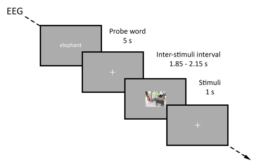
bioRxiv preprint first posted online Nov. 29, 2018; doi: http://dx.doi.org/10.1101/481630. The copyright holder for this preprint
(which was not peer-reviewed) is the author/funder, who has granted bioRxiv a license to display the preprint in perpetuity.
It is made available under a CC-BY-ND 4.0 International license.
A ERP difference B Single trial SVM classifier C Average category SVM classifier
P7 P7 P7
P4 P4 P4
Cz 20 Cz 20 Cz 20
Pz Pz Pz
P3 18
P3 18
P3 18
P8 P8 P8
O1 O1 O1
O2 16
O2 16
O2 16
T8 T8 T8
F8 F8 F8
C4 14
C4 14
C4 14
F4 F4 F4
Fp2 Fp2 Fp2
Fz 12
Fz 12
Fz 12
C3 C3 C3
F3 F3 F3
Fp1 10 Fp1 10 Fp1 10
T7 T7 T7
F7 F7 F7
Oz 8 Oz 8 Oz 8
PO3 PO3 PO3
AF3 AF3 AF3
FC5 6 FC5 6 FC5 6
FC1 FC1 FC1
CP5 CP5 CP5
CP1 4 CP1 4 CP1 4
CP2 CP2 CP2
CP6 CP6 CP6
AF4 2 AF4 2 AF4 2
FC2 FC2 FC2
FC6 FC6 FC6
PO4 0 PO4 0 PO4 0
-100 0 100 200 300 400 500 -100 0 100 200 300 400 500 -100 0 100 200 300 400 500
Time, [ms] Time, [ms] Time, [ms]
80 ms 210 ms 310 ms 330 ms 80 ms 210 ms 310 ms 330 ms 80 ms 210 ms 310 ms 330 ms
Fig. 3. Effect sizes for ERP animate/inanimate difference map and single-trial and average category SVM classifiers. Effect
sizes were computed based on 100 NPAIRS resampling splits.
Fig. 4. SVM classifier trained on average categories and tested on average categories. Significance estimated by permutation
testing.
gory classifier (Figure 3C). The average category classifier efficients in the range α = −7.2, . . . , 7.2, and 46 out of 345
exploited a larger proportion of earlier time points compared coefficients were zero (299 support vectors).
to the single-trial classifier. The sensitivity maps from the
single-trial and average category classifiers suggest that de-
spite the difference in number and type of trials, the classifiers 4. DISCUSSION
are similar.
In the current work, we approach the challenges of EEG-
The single-trial SVM classifier used for computing the based decoding: non-laboratory settings, user-friendly EEG
sensitivity map had model coefficients α = −1.5, . . . , 1.5, acquisition equipment with dry electrodes, naturalistic stim-
where 1204 α values out of 10350 were equal to 0 (9146 sup- uli, no repeated presentation of stimuli and no exclusion of
port vectors). The average category classifier had model co- participants. The potential benefits of mitigating these chal-bioRxiv preprint first posted online Nov. 29, 2018; doi: http://dx.doi.org/10.1101/481630. The copyright holder for this preprint
(which was not peer-reviewed) is the author/funder, who has granted bioRxiv a license to display the preprint in perpetuity.
It is made available under a CC-BY-ND 4.0 International license.
Fig. 5. Classifier trained on average categories (black) or trained on single trials (red) and tested on single trials. Note: In some
cases the ”optimum parameters” are not found to be optimum, which can be explained by different training phases of the two
single trial classifiers. The classifier based on validation sets was trained on 13 subjects while the classifier with parameters
based on the test set was trained on 14 subjects. For 5 out of 15 subjects the classifier based on 13 subjects was able to obtain
higher accuracies.
lenges is to study the brain dynamics in natural settings. 4.1. Event Related Potential Analysis
We aim to increase the EEG applicability in terms of Previous work on visual stimuli decoding demonstrate that
cost, mobility, set-up and real-time acquisition by using visual input reaches the frontal lobe as early as 40-65 ms
commercial-grade EEG equipment. Moreover, it has recently after image presentation and participants can make an eye
been demonstrated that commercial-grade EEG equipment movement 120 ms after onset in a category detection task.
compares to high-grade equipment in laboratory settings in Evidence of category specificity has been found at both early
terms of neural reliability as quantified by inter-subject cor- (∼ 150 ms) and late (∼ 400 ms) intervals of the visually
relation [Poulsen et al., 2017]. evoked potential [Rousselet et al., 2004, Rousselet et al.,
The stimuli in our experimental paradigm consisted of 2007]. ERP studies indicate that category-attribute interac-
complex everyday scenes and non-iconic views of objects tions (natural/non-natural) emerge as early as 116 ms after
[Lin et al., 2014], and animate and inanimate images were stimulus onset over fronto-central scalp regions, and at 150
similar in composition, i.e., an object or animal in its natural and 200 ms after stimulus onset over occipitoparietal scalp
surroundings. The presented images were therefore not close- regions [Hoenig et al., 2008]. For animate versus inani-
ups of animals/objects as in many previous ERP classification mate images, ERP differences have been demonstrated de-
studies, for instance when separating ”tools” from ”animals” tectable within 150 ms of presentation [Thorpe et al., 1996].
[Simanova et al., 2010, Murphy et al., 2011] or ”faces” from Kaneshiro et al., 2015, demonstrate that the first 500 ms of
”objects” [Kaneshiro et al., 2015]. single-trial EEG responses contain information for successful
Our ultimate goal is to decode actual semantic differences category decoding between human faces and objects, and
between categories; thus we perform low-level visual feature above chance object classification as early as 48-128 ms after
standardization on experimental trials prior to the experiment, stimulus onset [Kaneshiro et al., 2015].
investigate time dependency of the EEG response throughout However, there appears to be uncertainty whether these
the experiment (Figures S2-S3) and perform ASR to reduce early ERP differences represent low-level visual stimuli or ac-
this dependency. tual high-level differences. We observe the major differencebioRxiv preprint first posted online Nov. 29, 2018; doi: http://dx.doi.org/10.1101/481630. The copyright holder for this preprint
(which was not peer-reviewed) is the author/funder, who has granted bioRxiv a license to display the preprint in perpetuity.
It is made available under a CC-BY-ND 4.0 International license.
between animate/inanimate ERPs at around 310 ms (Figures task. We identified regions where discriminative information
2 - 3). Moreover, we find ERP signatures different among resides and found this information comparable to the differ-
subjects (comparable to [Simanova et al., 2010]), which chal- ence map between ERP responses for animate and inanimate
lenges the across-subject model generalizability with a sam- trials.
ple size of 15 subjects. While previous studies demonstrate that high-level cat-
egories in EEG are distinguishable before 150 ms after
stimulus onset [Rousselet et al., 2007, Hoenig et al., 2008,
4.2. Support Vector Machine Classification
Kaneshiro et al., 2015], we find the most prominent differ-
In this study, we adopted non-linear RBF kernel SVM classi- ence in animate/inanimate ERPs around 210 ms and 320 ms,
fiers to classify between animate/inanimate naturalistic visual which is also exploited by the SVM classifiers (Figure 3).
stimuli in a leave-one-subject-out approach. Based on the similarity between the effect size of sensi-
SVM classifiers have previously been implemented for tivity maps for single-trial and average category classifiers
EEG-based decoding. SVM in combination with independent (Figure 3), we conclude that these classifiers exploit the same
component analysis data processing has been used to classify EEG features to a large extent. Thus, we investigated whether
whether a visual object is present or absent from EEG [Stew- the average category classifier can successfully predict on
art et al., 2014]. Zafar et al., 2017, propose a hybrid algorithm single-trial subjects. We show that classifiers trained on av-
using convolutional neural networks (CNN) for feature ex- eraged trials perform at par with classifiers trained on a large
traction and likelihood-ratio-based score fusion for prediction set of noisy single-trial samples.
of brain activity from EEG [Zafar et al., 2017]. Taghizadeh- By linking temporal and spatial features of EEG to train-
Sarabi et al., 2015, extract wavelet features from EEG, and se- ing of SVM classifiers, we took an essential step in under-
lected features are classified using a ”one-against-one” SVM standing how machine learning techniques exploit neural sig-
multiclass classifier with optimum SVM parameters set sepa- nals.
rately for each subject. Prediction was performed based on 12
semantic categories of non-naturalistic images with 19 chan-
nel equipment [Taghizadeh-Sarabi et al., 2014]. 5. OVERVIEW SUPPLEMENTARY MATERIAL
We found very similar performance of the single-trial and
average trial classifiers (Figure 5). As the average classifier Appendix A: Sensitivity map Python code
is significantly faster to train, a full nested cross-validation Appendix B: Manual exclusion criteria for image selection
scheme was feasible. The fact that the two classifiers have
similar performance indicates that the reduced sample size in Supplementary file 1: Image IDs, supercategories and cat-
the average classifier is offset by these (averaged) samples egories for all images used in the experiment from Microsoft
better signal to noise ratio. The fast training of the average Common Objects in Context (MS COCO) image database.
trial classifier allows for parameter optimization and unbiased Figures S1-S9 contain supplementary material, and are
performance evaluation. used for reference in the main manuscript.
Based on the leave-one-subject-out classification perfor-
mance (Figures 4-5), it is evident that there is a difference
in how well the classifier generalizes across subjects, which 6. DATA AVAILABILITY
partly is due to the diversity of ERP signatures across sub-
jects (Figure S1). This can be explained by a manifestation of Code available:
inherent inter-subject variability in EEG. Across-participant https://github.com/gretatuckute/DecodingSensitivityMapping.
generalization in EEG is complicated by many factors: the
signal to noise ratio at each electrode is affected by the con-
tact to the scalp which is influenced by local differences in 7. CONFLICTS OF INTEREST
skin condition and hair, the spatial location of electrodes rel-
ative to underlying cortex will vary according to anatomical The authors declare that they have no conflicts of interest re-
head differences, and there may be individual differences in garding the publication of this paper.
functional localization across participants.
4.3. Sensitivity Mapping 8. FUNDING STATEMENT
In the current work, we ask which parts of the EEG signa- This work was supported by the Novo Nordisk Founda-
tures are exploited in the decoding classifiers. We investi- tion Interdisciplinary Synergy Program 2014 (Biophysi-
gated the probabilistic sensitivity map for single-trial and av- cally adjusted state-informed cortex stimulation (BASICS))
erage trial SVM classifiers based on a binary classification [NNF14OC0011413].bioRxiv preprint first posted online Nov. 29, 2018; doi: http://dx.doi.org/10.1101/481630. The copyright holder for this preprint
(which was not peer-reviewed) is the author/funder, who has granted bioRxiv a license to display the preprint in perpetuity.
It is made available under a CC-BY-ND 4.0 International license.
9. AUTHORS’ CONTRIBUTIONS 10. REFERENCES
G.T, N.P and L.K.H. designed research; G.T and N.P acquired [Andersen et al., 2017] Andersen, R. S., Eliasen, A. U., Ped-
data; D.S, G.T and N.P performed initial data analyses; G.T., ersen, N., Andersen, M. R., Hansen, S. T., and Hansen,
S.T.H and L.K.H performed research; G.T, S.T.H and L.K.H L. K. (2017). EEG source imaging assists decoding in a
wrote the paper. face recognition task. arXiv preprint arXiv:1704.05748.
[Cichy et al., 2014] Cichy, R. M., Pantazis, D., and Oliva,
A. (2014). HHS Public Access. Nature Neuroscience,
17(3):455–462.
[de Cheveigné and Arzounian, 2018] de Cheveigné, A. and
Arzounian, D. (2018). Robust detrending, rereferencing,
outlier detection, and inpainting for multichannel data.
NeuroImage, 172(December 2017):903–912.
[Delorme et al., 2007] Delorme, A., Sejnowski, T., and
Makeig, S. (2007). Enhanced detection of artifacts in eeg
data using higher-order statistics and independent compo-
nent analysis. Neuroimage, 34(4):1443–1449.
[Den Nationale Videnskabsetiske Komité, 2014] Den Na-
tionale Videnskabsetiske Komité (2014). Vejledning om
anmeldelse, indberetning mv. (sundhedsvidenskablige
forskningsprojekter). (Januar):116.
[Gerlach, 2007] Gerlach, C. (2007). A review of functional
imaging studies on category specificity. Journal of Cogni-
tive Neuroscience, 19(2):296–314.
[Güçlü and van Gerven, 2017] Güçlü, U. and van Gerven,
M. A. (2017). Increasingly complex representations of nat-
ural movies across the dorsal stream are shared between
subjects. NeuroImage, 145:329–336.
[Hoenig et al., 2008] Hoenig, K., Sim, E.-J., Bochev, V.,
Herrnberger, B., and Kiefer, M. (2008). Conceptual Flex-
ibility in the Human Brain: Dynamic Recruitment of Se-
mantic Maps from Visual, Motor, and Motion-related Ar-
eas. Journal of Cognitive Neuroscience, 20(10):1799–
1814.
[Huth et al., 2016] Huth, A. G., Lee, T., Nishimoto, S.,
Bilenko, N. Y., Vu, A. T., and Gallant, J. L. (2016). De-
coding the Semantic Content of Natural Movies from Hu-
man Brain Activity. Frontiers in Systems Neuroscience,
10(October):1–16.
[Huth et al., 2012] Huth, A. G., Nishimoto, S., Vu, A. T.,
and Gallant, J. L. (2012). A Continuous Semantic Space
Describes the Representation of Thousands of Object and
Action Categories across the Human Brain. Neuron,
76(6):1210–1224.
[Kaneshiro et al., 2015] Kaneshiro, B., Perreau Guimaraes,
M., Kim, H.-S., Norcia, A. M., and Suppes, P. (2015). A
Representational Similarity Analysis of the Dynamics of
Object Processing Using Single-Trial EEG Classification.
Plos One, 10(8):e0135697.bioRxiv preprint first posted online Nov. 29, 2018; doi: http://dx.doi.org/10.1101/481630. The copyright holder for this preprint
(which was not peer-reviewed) is the author/funder, who has granted bioRxiv a license to display the preprint in perpetuity.
It is made available under a CC-BY-ND 4.0 International license.
[Kay et al., 2008] Kay, K., Naselaris, T., Prenger, R., and [Peirce, 2009] Peirce, J. W. (2009). Generating stimuli for
Gallant, J. (2008). Identifying natural images from human neuroscience using PsychoPy. 2(January):1–8.
brain activity. Nature, 452(7185):352–355.
[Polich, 2007] Polich, J. (2007). Updating P300: An In-
[Lautrup et al., 1994] Lautrup, B., Hansen, L. K., Law, I., tegrative Theory of P3a and P3b. Clin Neurophysiol.,
Mørch, N., Svarer, C., and Strother, S. (1994). Massive 118(10):2128–2148.
Weight-Sharing: A Cure for Extremely Ill-Posed Prob-
lems. Workshop on Supercomputing in Brain Research: [Poulsen et al., 2017] Poulsen, A. T., Kamronn, S., Dmo-
From Tomography to Neural Networks, J{ü}lich, Ger- chowski, J., Parra, L. C., and Hansen, L. K. (2017). EEG
many, page 137. in the classroom: Synchronised neural recordings during
video presentation. Scientific Reports, 7:1–9.
[Lin et al., 2014] Lin, T. Y., Maire, M., Belongie, S., Hays,
J., Perona, P., Ramanan, D., Dollár, P., and Zitnick, C. L. [Prenger et al., 2009] Prenger, R. J., Gallant, J. L., Kay,
(2014). Microsoft COCO: Common objects in context. K. N., Naselaris, T., and Oliver, M. (2009). Bayesian re-
Lecture Notes in Computer Science (including subseries construction of natural images from human brain activity.
Lecture Notes in Artificial Intelligence and Lecture Notes Neuron, 63(6):902–915.
in Bioinformatics), 8693 LNCS(PART 5):740–755. [Rasmussen et al., 2011] Rasmussen, P. M., Madsen, K. H.,
[Lotte et al., 2007] Lotte, F., Congedo, M., Lécuyer, A., Lund, T. E., and Hansen, L. K. (2011). Visualization of
Lamarche, F., and Arnaldi, B. (2007). A review of clas- nonlinear kernel models in neuroimaging by sensitivity
sification algorithms for EEG-based brain-computer inter- maps. NeuroImage, 55(3):1120–1131.
faces. J. Neural Eng., 4(R1):R1–R13.
[Rousselet et al., 2007] Rousselet, G. A., Husk, J. S., Ben-
[Loula et al., 2018] Loula, J., Varoquaux, G., and Thirion, B. nett, P. J., and Sekuler, A. B. (2007). Single-trial EEG dy-
(2018). Decoding fmri activity in the time domain im- namics of object and face visual processing. NeuroImage,
proves classification performance. NeuroImage, 180:203– 36(3):843–862.
210.
[Rousselet et al., 2004] Rousselet, G. A., Mace, M. J.-M.,
[M Bishop, 2006] M Bishop, C. (2006). Pattern recognition and Fabre-Thorpe, M. (2004). Animal and human faces in
and machine learning. Springer-Verlag New York. natural scenes: How specific to human faces is the N170
ERP component? Journal of Vision, 4(1):2–2.
[Mullen et al., 2015] Mullen, T., Kothe, C., Chi, M., Ojeda,
A., Kerth, T., Makeig, S., Jung, T.-P., and Cauwenberghs, [Rowan and Tolunsky, 2003] Rowan, A. J. and Tolunsky, E.
G. (2015). Real-time Neuroimaging and Cognitive Mon- (2003). A primer of EEG: with a mini-atlas. Butterworth-
itoring Using Wearable Dry EEG. IEEE Transactions on Heinemann Medical.
Biomedical Engineering, 62(11):2553–2567.
[Saitta, 1995] Saitta, L. (1995). Support-Vector Networks
[Murphy et al., 2011] Murphy, B., Poesio, M., Bovolo, F., SVM.pdf. 297:273–297.
Bruzzone, L., Dalponte, M., and Lakany, H. (2011). EEG
decoding of semantic category reveals distributed rep- [Simanova et al., 2010] Simanova, I., van Gerven, M., Oost-
resentations for single concepts. Brain and Language, enveld, R., and Hagoort, P. (2010). Identifying object cat-
117(1):12–22. egories from event-related EEG: Toward decoding of con-
ceptual representations. PLoS ONE, 5(12).
[Nicolas-Alonso and Gomez-Gil, 2012] Nicolas-Alonso,
L. F. and Gomez-Gil, J. (2012). Brain computer interfaces, [Stewart et al., 2014] Stewart, A. X., Nuthmann, A., and
a review. Sensors, 12(2):1211–1279. Sanguinetti, G. (2014). Single-trial classification of EEG
in a visual object task using ICA and machine learning.
[Nishimoto et al., 2011] Nishimoto, S., Vu, A. T., Naselaris, Journal of Neuroscience Methods, 228:1–14.
T., Benjamini, Y., Yu, B., and Gallant, J. L. (2011). Recon-
structing visual experiences from brain activity evoked by [Strother et al., 2002] Strother, S. C., Anderson, J., Hansen,
natural movies. Current Biology, 21(19):1641–1646. L. K., Kjems, U., Kustra, R., Sidtis, J., Frutiger, S., Mu-
ley, S., LaConte, S., and Rottenberg, D. (2002). The
[Pedregosa et al., 2011] Pedregosa, F., Varoquaux, G., quantitative evaluation of functional neuroimaging exper-
Gramfort, A., Michel, V., Thirion, B., Grisel, O., Blondel, iments: The NPAIRS data analysis framework. NeuroIm-
M., Prettenhofer, P., Weiss, R., Dubourg, V., Vanderplas, age, 15(4):747–771.
J., Passos, A., Cournapeau, D., Brucher, M., Perrot, M.,
and Duchesnay, E. (2011). Scikit-learn: Machine learning [Taghizadeh-Sarabi et al., 2014] Taghizadeh-Sarabi, M.,
in Python. Journal of Machine Learning Research, Daliri, M. R., and Niksirat, K. S. (2014). Decoding Ob-
12:2825–2830. jects of Basic Categories from ElectroencephalographicbioRxiv preprint first posted online Nov. 29, 2018; doi: http://dx.doi.org/10.1101/481630. The copyright holder for this preprint
(which was not peer-reviewed) is the author/funder, who has granted bioRxiv a license to display the preprint in perpetuity.
It is made available under a CC-BY-ND 4.0 International license.
Signals Using Wavelet Transform and Support Vector
Machines. Brain Topography, 28(1):33–46.
[Thorpe et al., 1996] Thorpe, S., Fize, D., and Marlot, C.
(1996). Speed of processing in the human visual system.
Nature, 381.
[Zafar et al., 2017] Zafar, R., Dass, S. C., and Malik, A. S.
(2017). Electroencephalogram-based decoding cognitive
states using convolutional neural network and likelihood
ratio based score fusion. PLoS ONE, 12(5):1–23.bioRxiv preprint first posted online Nov. 29, 2018; doi: http://dx.doi.org/10.1101/481630. The copyright holder for this preprint
(which was not peer-reviewed) is the author/funder, who has granted bioRxiv a license to display the preprint in perpetuity.
It is made available under a CC-BY-ND 4.0 International license.
Supplementary materials
.1. Appendix A
The following piece of code shows how to compute the sensitivity map for a SVM classifier with an RBF kernel across all trials
using Python and NumPy (np).
map =
np.matmul(X,np.matmul(np.diag(alpha),k))-(np.matmul(X,(np.diag(np.matmul(alpha,k)))))
s = np.sum(np.square(map),axis=1)/np.size(alpha)
k denotes the (N × N ) RBF training kernel matrix from equation 2, with N as the number of training examples. alpha
denotes a (1×N ) vector with model coefficients. X denotes a (P ×N ) matrix with training examples in columns. s is a (P ×1)
vector with estimates of channel sensitivities for each time point, which can be re-sized into a matrix of size [no. channels, no.
time points] for EEG-based sensitivity map visualization.
.2. Appendix B
Manual exclusion criteria for MS COCO images [Lin et al., 2014] for the experimental paradigm:
- Object unidentifiable
- Object not correctly categorized
- Different object profoundly more in focus
- Color scale manipulation
- Frame or text overlay on image
- Distorted photograph angle
- Inappropriate imagebioRxiv preprint first posted online Nov. 29, 2018; doi: http://dx.doi.org/10.1101/481630. The copyright holder for this preprint
(which was not peer-reviewed) is the author/funder, who has granted bioRxiv a license to display the preprint in perpetuity.
It is made available under a CC-BY-ND 4.0 International license.
Animate
Inanimate
Subject 1 Subject 2 Subject 3 Subject 4 Subject 5
Scaled ERP amplitude [a.u.]
1 1 1 1 1
0.5 0.5 0.5 0.5 0.5
0 0 0 0 0
-0.5 -0.5 -0.5 -0.5 -0.5
-1 -1 -1 -1 -1
0 200 400 0 200 400 0 200 400 0 200 400 0 200 400
Subject 6 Subject 7 Subject 8 Subject 9 Subject 10
Scaled ERP amplitude [a.u.]
1 1 1 1 1
0.5 0.5 0.5 0.5 0.5
0 0 0 0 0
-0.5 -0.5 -0.5 -0.5 -0.5
-1 -1 -1 -1 -1
0 200 400 0 200 400 0 200 400 0 200 400 0 200 400
Subject 11 Subject 12 Subject 13 Subject 14 Subject 15
Scaled ERP amplitude [a.u.]
1 1 1 1 1
0.5 0.5 0.5 0.5 0.5
0 0 0 0 0
-0.5 -0.5 -0.5 -0.5 -0.5
-1 -1 -1 -1 -1
0 200 400 0 200 400 0 200 400 0 200 400 0 200 400
Time [ms] Time [ms] Time [ms] Time [ms] Time [ms]
Fig. S1. Animate and inanimate ERPs for each subject separately with two standard errors around the mean.bioRxiv preprint first posted online Nov. 29, 2018; doi: http://dx.doi.org/10.1101/481630. The copyright holder for this preprint
(which was not peer-reviewed) is the author/funder, who has granted bioRxiv a license to display the preprint in perpetuity.
It is made available under a CC-BY-ND 4.0 International license.
Fig. S2. Time dependency as quantified by autocorrelation. A high regression coefficient means that a channel (or an average
of all channels) had an autocorrelation which increased or decreased linearly with time lags, and is thus indicative of high time
dependency.
Fig. S3. Time dependency as quantified by variance of trials. A high regression coefficient means that a channel (or an average
of all channels) had a trial variance which increased or decreased linearly with trial number, and is thus indicative of high time
dependency.bioRxiv preprint first posted online Nov. 29, 2018; doi: http://dx.doi.org/10.1101/481630. The copyright holder for this preprint
(which was not peer-reviewed) is the author/funder, who has granted bioRxiv a license to display the preprint in perpetuity.
It is made available under a CC-BY-ND 4.0 International license.
Fig. S4. Validation accuracies (mean over validation sets) for the average category classifier. c values are displayed on the
x-axis, and consisted of values: [0.25, 0.5, 1, 1.5, 1.75, 2, 2.5, 5, 10, 15]. γ values are displayed on the y-axis, and consisted of
values: [5 × 10⁻⁷ , 2.5 × 10⁻⁶ , 5 × 10⁻⁶ , 2.5 × 10⁻⁵ , 5 × 10⁻⁵ , 2.5 × 10⁻⁴ , 5 × 10⁻⁴ , 2.5 × 10⁻³ , 5 × 10⁻³ , 2.5 × 10⁻² ].
Same scaling for all subjects.
Fig. S5. Test accuracies for average category classifier. Tested on the averaged categories of the withheld subject. Same
cross-validation parameter values as in Figure S4.
.bioRxiv preprint first posted online Nov. 29, 2018; doi: http://dx.doi.org/10.1101/481630. The copyright holder for this preprint
(which was not peer-reviewed) is the author/funder, who has granted bioRxiv a license to display the preprint in perpetuity.
It is made available under a CC-BY-ND 4.0 International license.
Fig. S6. Test accuracies for average category classifier. Tested on the individual trials of the withheld subject. Same cross-
validation parameter values as in Figure S4.
Fig. S7. Cross-validation with a single held out subject to estimate parameters for the upper level per-
formance single-trial SVM classifier. c values are displayed on the x-axis, and consisted of values:
[0.05, 0.25, 0.5, 1, 1.5, 1.75, 2, 2.5, 5, 10]. γ values are displayed on the y-axis, and consisted of values:
[2.5 × 10⁻⁷ , 5 × 10⁻⁷ , 2.5 × 10⁻⁶ , 5 × 10⁻⁶ , 2.5 × 10⁻⁵ , 5 × 10⁻⁵ , 2.5 × 10⁻⁴ , 5 × 10⁻⁴ , 2.5 × 10⁻³ , 5 × 10⁻³ ].bioRxiv preprint first posted online Nov. 29, 2018; doi: http://dx.doi.org/10.1101/481630. The copyright holder for this preprint
(which was not peer-reviewed) is the author/funder, who has granted bioRxiv a license to display the preprint in perpetuity.
It is made available under a CC-BY-ND 4.0 International license.
Fig. S8. Upper level performance parameters for the single-trial SVM classifier based on the mean parameters for held out
subjects in Figure S7.
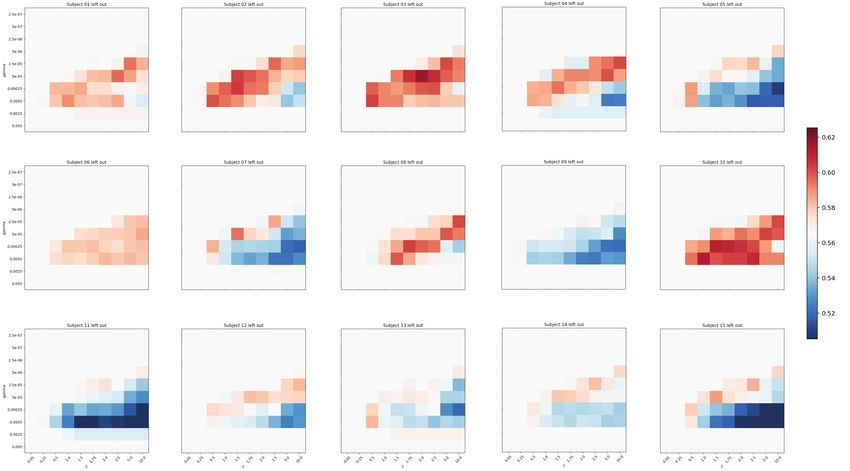
Fig. S9. Optimum parameters for the single-trial SVM classifier based on the mean parameters of validation partition 1 (subjects
1-7) and partition 2 (subjects 8-15). Same cross-validation parameter values as in Figure S4.You can also read