Spectral Efficiency of Dynamic Licensed Shared Access

Page created by Derrick Gonzales
 
CONTINUE READING
Spectral Efficiency of Dynamic Licensed Shared Access
1

     Spectral Efficiency of Dynamic Licensed Shared
                          Access
                Samuel Onidare, Keivan Navaie, Senior Member, IEEE, Qiang Ni, Senior Member, IEEE

   Abstract—In licensed shared access (LSA) the radio spectrum                solution to the challenge of additional spectrum requirement
is dynamically shared between an incumbent and one or more                    in the sub - 6 GHz 5G technology space [4]–[10].
licensee systems. Protective measures are then applied to the                    The LSA framework as specified in [11], while ensuring
licensees’ communication activity to protect normal operation
of the incumbent system. Such measures are therefore crucial                  provision of a predictable quality of service (QoS) to nodes on
components of the LSA, and thus fundamentally affect the                      the LSA licensee network, also demands guarantee of protec-
achievable spectrum efficiency. In this paper we investigate a                tion against harmful interference to the incumbent. Guarantee-
vertical LSA including an airport traffic control system, as                  ing such protection necessitates an exclusion zone which could
the incumbent, and a mobile network as the licensee. Unlike                   lead to a significant spatial under-utilization of the spectrum
some previous works that only consider the licensee uplink, we
analytically obtain the interference received by the incumbent                [12], [13]. To overcome this inefficiency, a less restrictive and
from the licensee’s transmission both in the uplink and downlink.             dynamic exclusion zone becomes necessary. This is more so
We then obtain optimal uplink and downlink power allocation                   considering the fact that the initial frequency band proposed
in the licensee using an optimisation problem with the objective              for the LSA under the European communication commission
of maximizing licensee’s spectral efficiency (SE) subject to the              (ECC) harmonization, the 2.3 GHz- 2.4 GHz, is presently
incumbent interference threshold. Furthermore, we investigate
the effect of the number of users and cell size on the SE. Our                occupied by services such as the aeronautical and terrestrial
results provide quantitative insights for practical system design             telemetry [11]. It should also be noted that this frequency band
and deployment of LSA system. We then examine the whole LSA                   is an initial proposal for harmonization by the ECC and can
spectrum utilization by characterising the availability of the LSA            differ from one country to another depending on the spectrum
spectrum using a tandem queue setting. Using this model we                    utilization in each country [14]. Furthermore, the possibility
obtain an expression for the spectral utilization as a function
of the licensee’s achievable spectral efficiency and the statistics           of using the 3.8 GHz has been proposed for the authorised
of the LSA spectrum availability. Simulation results show more                shared access, the concept on which the LSA was based [11].
than a seven-fold improvement in the licensee SE using the                       Considering a scenario, where the incumbent is an airport,
optimal power allocation. It is also seen that a higher SE gain               and the licensee is a mobile network operator (MNO), teleme-
is achieved with the proposed optimal power allocation in cases               try communication between the airport traffic control (ATC)
where the number of user equipment in the eNodeB coverage
area is very small. Furthermore, higher spectrum utilization                  and the flying airplane can only be affected by the licensee
efficiency is achieved as a result of shorter busy period and higher          transmission within a small portion of the exclusion zone
achievable SE for distant cells.                                              and for a significantly small period of time. As a result, the
   Index Terms—Spectrum efficiency, dynamic licensed shared ac-               ATC transmission with the flying aircraft can only experience
cess, spectrum utilization, interference threshold, tandem queue              significant interference from the MNO activities within the
                                                                              flight trajectory if and only if, the telemetry transmission ‘radio
                                                                              shadow’ radius crosses the MNO cell border [15]. Based on
                                                                              this scenario, the European Union (EU) regulatory framework
                         I. I NTRODUCTION
                                                                              proposes a dynamic form of LSA [16].
   As we enter the zettabytes era of internet data traffic [1],                  On the basis of this framework, authors in [17], develop
spectrum access approaches must evolve to address the ac-                     algorithms for spectrum allocation in dynamic LSA. It is
companying challenges. In this regard, the licensed shared                    also shown in [13] that the dynamic LSA can be achieved
access (LSA) becomes imperative for spectrum access. In                       by either shutting-down licensee’s communications or re-
LSA the radio spectrum is dynamically shared between an                       ducing its transmission power to a tolerable level for the
incumbent and one or more licensee systems. The flexibility                   incumbent system where and when the incumbent system is
in spectrum management provided by the LSA makes it a                         active. Simulation results in [13] further indicate that limiting
suitable solution to address the demand for high density                      transmission power as in [18] results in SE degradation. An
machine type communication [2] as well as providing back                      experimental confirmation of the viability of the dynamic LSA
up solution to unexpected network down time especially for                    is then carried out using a commercial grade LTE testbed
public safety purposes during disaster outbreaks and for rescue               in [4]. Similarly, the work in [9], determined the protection
operations [3]. Several experimental field trials with live long              criteria for the LSA operation between a MNO licensee and
term evolution (LTE) also suggest that LSA provides a viable                  a programme making and special events (PMSE) incumbent
                                                                              system. Experimental demonstrations in [19] further verifies
  Authors are with the School of Computing and Communications, Lancaster
University, Lancaster LA1 4WA, U.K. This research was also partly supported   the feasibility of the licensee’s compliance with the regulatory
by H2020-MSCA-RISE-2015 ATOM 690750.                                          requirements of various incumbent systems.
2

   In [18], a mathematical formulation is provided to analyse      function of the achievable SE and the ratio of the busy period
applying limiting transmit power policy in dynamic LSA.            of each service layer (eNodeB coverage) to the busy period
Using queueing theory and Markov process, [18], [20]–[22]          of all the service layers in the tandem queue. This is more so,
then investigate performance of LSA using metrics such as          considering the fact that the challenge of spectrum scarcity
service interruption and blocking probability, average number      was as a result of inefficiency in the spectrum utilization.
of connected users, service failure and mean bit rate. In          Furthermore, in view of the envisaged future capacity demand,
[19], it is further demonstrated that the radio environment        we also investigate optimization of the LSA throughput.
map (REM) can be used to detect the specific area of the              The main contributions of this paper are summarised in the
incumbent’s activity in a dynamic LSA system. In [23], the         following:
authors proposed a QoS aware resource allocation and caching          • We derive expression for the interference received by the
for a spectrum sharing between terrestrial satellite system and          incumbent from the licensee’s transmission both in the
a cellular network. Different scenarios where the LSA can be             uplink and downlink. Similar to [13], [18], our previous
deployed for capacity increase in the 5G technology space                work in [28], only considers the licensee’s uplink in the
as well as a new architecture and enabling technologies were             analysis.
presented in [24]. The work in [25] focuses on the enforcement        • The effect of various operational parameters (i.e., the
of compliance by all parties in the LSA to the sharing rules             number of UEs in licensee coverage area, the eNodeB
by proposing a framework that discourages licensees from                 coverage radius and the adopted eNodeB transmit power)
flouting the rules.                                                      on the SE is also examined. Our results provide quantita-
   As it is seen the common theme of the aforementioned                  tive insights for practical system design and deployment
existing works is their focus on the incumbent’s protection,             of LSA system.
although without giving adequate attention to the licensee’s          • We introduce a novel performance measure, “decibel
network optimization. This is the main motivation of [26]                capacity gain” to quantify the improvement obtained by
that shows optimizing LSA resources and better spectrum                  the proposed power allocation technique. Using decibel
utilization can be achieved while ensuring incumbent’s pro-              capacity gain we further investigate the SE gain pattern
tection from excessive interference with licensee transmit               which shed light on the relation of SE to the number of
power reduction and antenna downward tilt adjustment. The                UEs and transmit power adjustment.
optimization in [26] focuses on the optimal number of cells           • Finally, we propose a novel formulation of the LSA spec-
that needs to be shut down in order to comply with the                   trum utilization efficiency as a function of the achievable
interference threshold constraint in the incumbent system                SE and busy period ratio of each layer (eNodeB coverage
within a geographical area. In [27], it is demonstrated that             area) to all the service layers (all eNodeB coverage area)
using opportunistic beamforming for resource allocation and              within the tandem queue, i.e., the considered geographical
scheduling of the licensee system in a LSA setting with                  radius around the incumbent.
horizontal spectrum sharing between two MNOs, the overall             Simulation results show more than a seven fold improve-
throughput of both networks can be improved.                       ment in the licensee achievable SE compared to a non-
   Against this background, in this paper we examine a vertical    optimized system. It is also seen that a higher comparative SE
LSA sharing between an airport traffic control system as the       gain is achieved with the proposed optimal power allocation
incumbent and a MNO as the licensee. Specifically we focus         in cases where the number of user equipment in the eNodeB
on improving the licensee’s system throughput, where the           coverage area is very small. Furthermore, higher spectrum
incumbent is utilizing the spectrum for telemetry services. Un-    utilization efficiency is achieved as a result of shorter busy
like some previous works that have only examined the licensee      period and higher achievable SE for distant eNodeB coverage.
uplink, we consider both the uplink and downlink transmis-
                                                                      The rest of this paper is organised as follows. In Section II,
sion directions. We begin by an analysis of the interference
                                                                   we present the system model and mathematical formulation. In
from the eNodeB to the the ATC tower as a result of the
                                                                   Section III, we optimise the spectral efficiency of the licensee
licensee downlink transmission followed by the interference
                                                                   in both downlink and uplink spectrum, and obtain the optimal
from the user equipment (UEs) to both the ATC tower and
                                                                   power allocation. Then in Section IV we present the spectrum
the aircraft(s). We then impose the incumbent interference
                                                                   availability model as a tandem queue and define a novel
threshold on the licensee system’s maximum achievable SE
                                                                   spectrum utilization metric as a function of the optimal SE
and obtained optimal power allocation for the downlink and
                                                                   and average spectrum busy period. Section V, discusses the
uplink transmission. We further examine the effect of various
                                                                   simulation results and analysis, followed by conclusions in
operational parameters that are critical to practical cellular
                                                                   Section VI.
network design and deployment.
   Furthermore, we examine the achievable LSA spectrum
utilization efficiency within a geographical radius of about                            II. S YSTEM M ODEL
200 km while employing limited licensee’s transmit power             We consider a circular area with a radius similar to the
to ensure protection against harmful interference to the in-       exclusion zone radius for an airport incumbent. Furthermore,
cumbent system. To do this, we characterize the availability       we assume the LSA licensee, a Mobile network Operator
or not of the LSA spectrum as a tandem queue and then              (MNO), has multiple cells of radius R within the considered
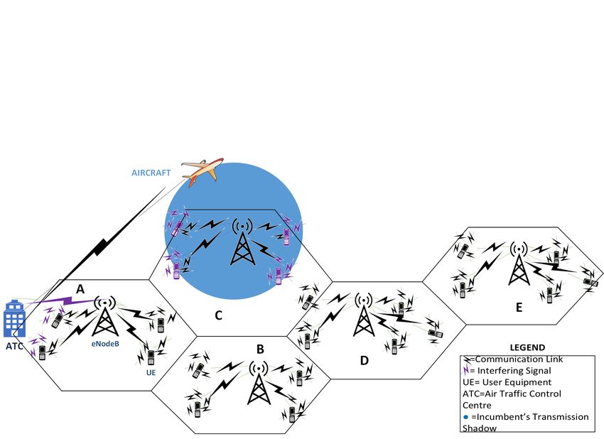
derive an expression for the utilization efficiency as a utility   geographical radius (Fig. 1). The incumbent uses the spectrum
3

Fig. 1: A schematic of the considered system: Incumbent’s transmission shadow only crosses licensee cell C, while cells A,
B, D, and E are outside the transmission shadow.

specifically when the ATC system is communicating with the                A. Incumbent’s Received Interference
aircraft(s). In this time period, the spectrum is considered as              In this section, we consider the interference that could
busy/unavailable. The rest of the time, the spectrum is referred          impair the ATC transmission to the flying aircraft during the
to as free and available for the MNO unrestricted access.                 take-off or landing. Here we consider two cases. The first case
   We further assume a multi-carrier transmission model, e.g.,            corresponds to the eNodeB coverage, see cell A in Fig. 1,
a LTE system with multiple-antenna eNodeB communicating                   where the interference to the incumbent’s system comprises
with single-antenna user equipment (UEs), is deployed by the              of rather strong interference signals from eNodeBs and less
MNO licensee. The channel gain vector for k user equipment                strong but multiple interfering signals originating from the
is represented as gk = [gk1 , . . . , gkΛ ], where k = 1, 2, . . . , K,   UEs. We consider the effect of this interference on the ATC
and Λ is the number of transmitting antenna. The channel                  tower and the aircraft with the assumption that there is perfect
input-output relationship is therefore:                                   co-operation and synchronization between the licensee and the
                                                                          incumbent operation that ensures no cross- slot interference.
                                                                             The second case is where the incumbents’ interference is
                          Xk = gk P + N,                           (1)    only comprised of signals from the UEs. It is reasonable to
                                                                          assume that a critical network design consideration of an LSA
                                                                          licensee is to ensure that the eNodeB antenna height is suffi-
where Xk is the channel output, P = [P1 , . . . , PΛ ] is the             ciently low relative to the ATC tower with a directional pattern
transmit power vector, and N is the complex noise, for the k th           (directed downwards to the UEs). Hence, omni-directional
UE. For easy referencing, the symbols used in this paper are              transmissions of UEs becomes the main components of the
given in Table I. Similar to the ATC communication system,                interfering signal [13]. Moreover, for distant licensee cells,
the licensee uses a time division duplexing (TDD) system.                 i.e., where the ATC tower is outside the eNodeB coverage
Furthermore, we also assume that the transmission link from               area, the incumbents received interference only includes UEs’
the ATC tower to the aircraft uses the same channel as the                signals within the incumbent’s transmission shadow radius.
MNO uplink transmission and equivalently the reverse link,                This is shown in eNodeB coverage area C of Fig. 1.
i.e., from the aircraft to the ATC tower, uses the same channel              1) Interference from the Licensee eNodeB Here we assume
as the MNO downlink.                                                      the licensee’s eNodeB is at least of a comparable height and
4

                  TABLE I: List of Parameters                                     2) Interference from Licensee UE Another, more likely,
     Parameter   Description                                                   source of interference to the incumbent system is the omni
     Q           Number of tandem queue service layers                         directional transmission in the uplink direction of the licensee
     γ −1        Time between successive flight take-off or landing(s)         system. The interference from this source comprises of in-
     µ−1         Time of ATC communication with an aircraft                    terfering signals from the UEs to both the uplink (airplane
     τ −1        Duration of the spectrum vacancy(s)                           receiver) and the downlink (ATC tower receiver) of the in-
     s           LSA spectrum status                                           cumbent system, in contrast to the interference signal from
     J           Number of aircraft landings at or take-offs                   the eNodeB which only affects the downlink transmission
     k           Individual UE                                                 of the aeronautic telemetry system. This is based on the
     yk          Location of individual UE                                     assumption that the eNodeB uses antennas with directional
     ya          Location of aircraft                                          radiation pattern directed downwards to the mobile stations
     n           Path loss exponent                                            [13]. We consider K UEs, each independently and randomly
     Λ           No of transmitting antenna                                    located at location x within the coverage area of eNodeB.
     Pk          Transmission power                                            The spatial distribution of the UEs in the coverage area of the
     l           Distance related power loss                                   eNodeB can then be characterised by a Poisson point process
     r           Distance between the ATC transceiver and the MNO              as the following:
                 interferer
     gd          Ground/horizontal distance between the aircraft and                                ϕ = {x1 , x2 , ......xK } .               (4)
                 a user equipment
     vd          Vertical distance/height between the aircraft and a
                 user equipment
                                                                               Therefore, the cumulative interference to the incumbent sys-
     D           Radius of the interference circular area                      tem at a point y as a result of the licensee UEs transmission
     Ith         Incumbent interference threshold                              is:
     G           Propagation constant                                                   X
     gk          Sub-channel gain vector                                           IK =     Pk Hk l(ky − xk k),       k = {1, 2, . . . , K} (5)
     K           Sub-channel set                                                         x∈ϕ

     P           transmit power vector
                                                                               where Pk , the UE transmission power, is Bernoulli distributed
     H           Channel gain vector
                                                                               with parameter p = Pr{Pk = 1} as the probability that
     ηSE         Spectrum efficiency
                                                                               each of the expected K UEs is transmitting, Hk the fading
     L           Lagrange multiplier
                                                                               coefficient is an exponential random variable. In theory, the
     R           eNodeB cell radius
                                                                               MIMO antenna system allows more than one UE transmitting
     nUE         No. of user equipment
                                                                               at the same time, but currently in practice, it is still being used
     λ           Poisson node distribution density
     N           Noise power
                                                                               primarily for eNodeB simultaneous transmissions to several
                                                                               UEs. Furthermore, the PHY and MAC layers of LTE try to
                                                                               avoid all simultaneous transmissions from UEs connected to
                                                                               a single eNodeB. We can therefore assume that even though
possibly on the same horizon with the ATC tower. Although
                                                                               there could be many UEs per eNodeB, there is no more than
careful network design should ensure that the likelihood of
                                                                               one UE per eNodeB transmitting simultaneously.
this scenario playing out is very low but it is a possibility that
is worth considering. Thus, the interference from a licensee’s                    We then define distance ky − xk k, (x ∈ ϕ), as krk ≤ D,
eNodeB located at a distance r to the ATC tower is:                            and the intervening area between the UEs is represented as a
                                                                               ball b(y, D), centred at y and of radius D. The interference
                          IB = PB hB l(r),                               (2)   point process ϕI = ϕ ∩ b(y, D) is then defined similar to the
                                                                               inner city model of the Cox process [29], where ϕI , and ϕ
where, IB is the licensee eNodeB interference power, PB , hB ,                 are Poisson processes with density λI , and λ, respectively, and
is the eNodeB transmit power and fading component respec-                      λI = λcd drd−1 , where, cd = kb(0, 1)k is the volume of d-
tively, l(r) is the path loss as a result of the separation distance           dimensional unit radius ball. The probability density function
d between the eNodeB and the ATC tower and is given by                         of the interference point process ID is therefore
l(r) = krk−n , n is the path loss exponent. In cases where                                        ∞          k
there are more than one eNodeB within interfering range of the                                 1 X Γ(βk + 1) ρ
                                                                                  fID (i; β) =                   sin kπ(1 − β),               (6)
ATC tower, the aggregate interference from multiple eNodeBs                                    πi     k!     iβ
                                                                                                   k=1
is:
                                                                                           2
                                                                               where β =   n,   Γ(.) is gamma function, and ρ = λI πΓ(1 − β).
                                  "N         #
                                     XB

                  IAGB = 10 log          IB + 30,                (3)
                                      B=1
                                                                               B. The Interference Propagation Path
where IAGB is the aggregate interference to the ATC tower
from multiple eNodeBs in dBm (hence adding 30 in the                             Following the same line of argument as in II-A, we char-
above), NB is the number of interfering eNodeBs, and IB                        acterize the propagation path for the interference due to the
is the individual eNodeB interference power in Watts.                          eNodeB as well as the interference due to the UEs.
5

        TABLE II: Parameters for Pr{LoS, θ} in (9).                     or as a function of the aircraft altitude and the
                                                                        ground/horizontal distance of the UEs:
      Environment         a       b         c      d        e
                                                                                                                     vd2
                                                                                                                        
      Suburban          101.6     0         0     3.25    1.241
      Urban             120.0     0         0    24.30    1.229         PL(vd , gd ) = 20 log(gd ) + 10 log 1 + 2 + k + ζnLoS + lb
                                                                                                                     gd
      Dense Urban       187.3     0         0    82.10    1.478                                                      
      Urban High-Rise   352.0   -1.37      -53   173.80   4.670                                       a−b
                                                                                     +A a −                 v           ,  if gd > vd ,
                                                                                                    tan−1 ( gd )−c e
                                                                                              1+          d
                                                                                                             d

                                                                                                                                 (11a)
   1) Air-to- Ground Pathloss Model The path between the                                                      
                                                                                                                     g2
                                                                                                                         
UE interferers and the flying aircraft is analogous to the air          PL(vd , gd ) = 20 log(vd ) + 10 log 1 + d2 + k + ζnLoS + lb
                                                                                                                     vd
to ground channel model. According to [30], the transmitter–                                                         
receiver path/air to ground channel (ATG) can be characterised                                        a−b
                                                                                     +A a −                 v           ,  if gd ≤ vd ,
                                                                                                    tan−1 ( gd )−c e
as:                                                                                           1+             d
                                                                                                          d
                     PL =
                           X
                               PLg Pr{g, θ},               (7)                                                                   (11b)
                            g                                           where gd is the horizontal distance of the UEs in km, vd , is
                                                                        the altitude of the aircraft also in km, k = 20 log(f ) + 92.4,
where PL, stands for the path loss between the aircraft and the         f is the carrier frequency in GHz, and A = ξLoS − ξnLoS .
ground receivers or UEs, g ∈ {LoS, NLoS}, is the propagation               2) Extended Hata Model In line with the recommendation
group, where LoS and NLoS are the line of sight and non                 contained in the report by the U. S. department of commerce,
line of sight propagation respectively. In (7), Pr{g, θ} is the         National Telecommunication and Information Administration
probability of LoS and NLoS, θ is the elevation angle between           (NTIA) in [34], we use the extended Hata model (eHata) for
a ground UE and the aircraft, and                                       the signal attenuation along the path between the licensee
                                                                        eNodeB and the ATC tower as well as the propagation path
                        PLg = FSPL + ξg .                         (8)   between the UEs and the ATC tower. The model is valid for
                                                                        frequency range from 1500–3000 MHz, distance of 1–100
In (8) FSPL is the free space path loss and ξ is the excessive          km, transmitter and receiver height of 30–200 m and 1–10
path loss, which is, propagation group (LoS or NLoS) and                m respectively. Therefore, the eHata point to point median
environment dependent. Note that ξLoS , can be approximated             basic transmission loss for an urban outdoor environment is:
by a log-normal distributed with location variability parameter
                                                                        PLeH (f, r, hB , hR )
ζLoS [31], while for the ξnLoS , an additional building roof                                              
                                                                                                                            
top diffraction loss lb [32] is factored into the equation, i.e.,                                     r                   200
                                                                           = Lbm (f, Rbp ) + 10n log        + 13.82 log
ξnLoS = ζnLoS + lb .                                                                                 Rbp                  hB
                                                                                                                   
   Using the ITU-R recommendations P-1410 [33], Pr{g, θ}                    +v(3) − v(hR ) + PLfs f, R(r, hB , hR ) ,
for LoS propagation is obtained in [32] as:                                                                                   (12a)

                                           a−b                              Lbm (f, Rbp ) = 30.52 − 16.81 log f
                Pr{LoS, θ} = a −                     ,            (9)                                                                      (12b)
                                        1 + ( θ−c  e                      +4.45(log f )2 + (24.9 − 6.55 log hB ) log Rbp ,
                                               d )
                                                                          v(hR ) = (1.1 log f − 0.7)hR − 1.56 log f + 0.8,                   (12c)
where a, b, c, d, and e, are parameters obtained from extensive
simulations and presented in ITU-R recommendations P-140
                                                                                              p
                                                                          R(r, hB , hR ) = (r × 103 )2 + (hB − hR )2 ,                       (12d)
[33] and experimentally validated in [32]. Table II presents the
                                                                                                                      1
values obtained from the experiment.
                                                                                                               ! (n −n
                                                                                                                    h   l)
                                                                                        2nh lbm (f, 1)                                       (12e)
   Substituting FSPL, (8),(9) into (7)p and noting that                   Rbp = 10                                         ,
                                                                                             lbm (f, 100)
transmitter-to-receiver distance is r =       vd2 + gd2 , we then
                                                                                
express the path loss as a function of elevation angle:                             0.1(24.9 − 6.55 log hB ) for 1km ≤ r ≤ Rbp ,
                                                                           n=       2(3.27 log h  − 0.67(log h )2 − 1.75)d, for R ≤ r ≤ 100km,
                                                                                                B           B               bp

PL(θ) = 20 log(gd ) + 10 log 1 + (tan θ)2 + k + ζnLoS + lb
                                          
                                                                                                                        (12f)
                                                              and Lbm is the basic median attenuation relative to free space,
                                       
                               a−b
                   +A a −                ,   if gd > vd ,     r is the transmitter-receiver separation distance, Rbp is the
                            1 + ( θ−c
                                   d )
                                      e

                                                     (10a)    breakpoint distance, hB and hR is the transmitter and receiver
                                                              antenna height respectively, v(hR ) is the receiver’s reference
                                                            height correction factor, PLfs is the free space path loss at
                                      1
PL(θ) = 20 log(vd ) + 10 log 1 +             + k + ζnLoS + lb distance R, f represents the transmission frequency, nh and
                                  (tan θ)2                    nl are the transmitter’s effective height dependence of the
                                         
                                 a−b                          higher and lower distance path loss exponent of the median
                     +A a −                ,    if gd ≤ vd ,
                              1 + ( θ−c e                     attenuation relative to free space respectively, and lbm is the
                                     d )
                                                       (10b)  frequency  extrapolated basic median transmission relative to
6

free space. For a suburban outdoor environment the eHata                         s.t.   PB HB l(r) ≤ Ith .
Pathloss model is,                                                                                                                (16b)
                                                       2              In (15) and (16), (15b) and (16b), are the constraint on the total
PLeHs = PLeH − (54.19 − 33.30 log f + 6.25(log f) ),
                                                                      interference from the licensee’s transmissions in the uplink,
                                                              (13)
                                                                      and downlink, respectively, and Ith represents the incumbent’s
where PLeHs is the eHata Pathloss model for the suburban              interference threshold, i.e., the maximum allowed interference
environment and PLeH is its urban equivalent presented in             for incumbents safe operation.
(12a)- (12f). Due to the large distance between the MNO                  Since in the uplink, the interference constraint is imposed
interferers (eNodeB and UEs), and the ATC transceivers (ATC           by multiple randomly distributed sources, to solve (15), the
tower and the aircraft), we model the fading component as a           sum constraint on the Pinterference power is decomposed as in
log normal random variable to capture the effect of large scale                                 K
                                                                      [35], such that Ith = k=1 Ithk . Thus (15) is rewritten as:
fading.
                                                                                             K
                                                                                             X                    
                                                                          ∗
      III. L ICENSEE S YSTEM S PECTRUM E FFICIENCY                       ηSE = max                 log2 1 + PU k gk ,                          (17a)
                                                                                        PU
                                                                                             k=1
   We assume that perfect channel state information (CSI) is
available at the transmitter. In cases where the incumbent sys-                    K                                       K
tem is not utilizing its spectrum, the licensee is able to transmit
                                                                                   X                                       X
                                                                         s.t.            PU · Hk · PL(vdk , gdk ) −               Ithk ≤ 0,
at maximum power to guarantee the desired signal to noise                          k=1                                    k=1
ratio (SNR) for each UEs according to its QoS requirement.                                                                                     (17b)
In our model, the users are assumed to be randomly distributed
                                                                                 PU k > 0               {k = 1, 2, ......, K}.                 (17c)
according to (4) within the eNodB coverage area, thus the total
system SE, ηSE , is the summation of the achievable bit rate          Using PB =
                                                                                         PK
                                                                                                   PBk , (16) is transformed to
                                                                                             k=1
for K UEs,
                           K
                                                                                                 K
                          X                  
                   ηSE =      log2 1 + Pk gk ,                 (14)                              X                   
                                                                             ∗
                                                                            ηSE = max                  log2 1 + PBk gk ,                       (18a)
                            k=1                                                          (PB )
                                                                                                 k=1
where gk is the channel gain to noise ratio.
                                                                                                                        K
                                                                                                                        X
A. Maximizing the Licensee Spectrum Efficiency                                  s.t.    HB ·PLeH (f, r, hB , hR )·            PBk −Ith ≤ 0, (18b)
                                                                                                                        k=1
   If the LSA spectrum is unavailable, the licensee has to
limit its transmit-power to ensure that the total interference
                                                                                        PBk > 0                 {k = 1, 2, ......, K} .        (18c)
power of the licensee (the MNO) at the incumbent receiver
does not exceed the interference threshold. In other words, the
transmit power should be reduced such that the incumbent’s               In (17) and (18), (17c) and (18c) are the non-negative
outage probability, 1 − Ps {θ}, does not exceed a given               allocated power constraints for the uplink and downlink,
performance threshold, θ, where Ps {θ}) = Pr{SINR > θ} is             respectively, and the corresponding optimization decision vari-
the transmission success probability. Thus, while maximizing          ables are PU = [PU 1 , . . . , PU K ] and PB = [PB1 , . . . , PBK ].
the achievable SE, the sum transmit power of the licensee must        Furthermore, PL(vdk , gdk ) is the path loss for the air -to-
be such that the total interference caused to the incumbent does      ground channel as a function of the height difference vdk and
not cause outage.                                                     horizontal separation gdk between the k th UE and the aircraft
   To facilitate performance evaluation, and to differentiate         while PLeH (f, r, hB , hR ) stands for the path loss between
uplink and downlink transmissions in our analysis we define           the eNodeB and the ATC tower as a function of the carrier
PU k for the transmit power of the k th UE in the uplink, and         frequency f , transmitter-receiver separation r between them,
equivalently PBk for the fraction of the eNodeB downlink              hB is the eNodeB antenna height and hR is the ATC tower
transmitted power to the k th UE. Therefore, maximizing SE            antenna height.
for the uplink is formulated as the following:                           Using the Lagrangian method, we have:
                     K
       ∗
                     X                                              L(PU k , λ, vk ) =
      ηSE = max            log2 1 + PU k gk ,                (15a)                               K
                                                                                                                              !
              PU                                                                                 X
                     k=1
                                                                                                       log2     1 + PU k gk
              K
              X                                                                                  k=1
       s.t.         PU k Hk l(rk ) ≤ Ith ,                                                       K 
                                                                                                 X                                            !
              k=1                                                                       −λ              PU k · Hk · PL(vdk , gdk ) − Ithk
                                                             (15b)                               k=1
and for the downlink as:                                                                          K
                                                                                                  X
                     K
                     X                                                                     +         v k PU k ,
       ∗
      ηSE = max            log2 1 + PBk gk ,                 (16a)                               k=1
               PB                                                                                                                                  (19)
                     k=1
7

and for the downlink                                                              Following similar steps, the solution to the optimization
                                                                                  problems in (15)-(17), yields the equivalent optimal power
L(PBk , λ, vk ) =                                                                 allocation in the downlink transmission direction as
                     K
                                                   !
                     X                                                                        "                                        #
                            log2      1 + PBk gk                                        ∗                      1                    1
                                                                                      PBk =                                    −      ,
                     k=1
                                                                                !               λ ln(2) HB PLeH (f, r, hB , hR )   gk     (24)
                                                              K
                                                              X
                     −λ HB · PLeH (f, r, hB , hR ) ·                PBk − Ith                                                                   ∀k ∈ K.
                                                              k=1
                     K                                                                In order to find the optimal allocated power Pk∗ , in a
                     X
                 +         vk PBk ,                                                situation where some channels have a non positive allocated
                     k=1                                                           power, we need to define and redistribute the available power
                                                                          (20)     to a set Kp ⊂ K that contains strictly non-negative power
                                                                                                                                           ∗
                                                                                   allocations. In this case the optimal allocated power, P{U,B}k ,
where λ ≥ 0 and vk ≥ 0 are Lagrangian multipliers for the                          becomes
interference and non negative power constraint. For the sake                                 "                                   #
of brevity we will forthwith proceed with the solution of the                           ∗                    1                 1
                                                                                      PU k =                            −       ,
uplink alone. Consequently, the Karush Kuhn Tucker (KKT)                                       λ ln(2) H PL(v , g )           gk              (25)
                                                                                                                   k     dk     dk
conditions [36] are:
                                                                                                                                      ∀k ∈ Kp |Pk > 0,

      δL                              gk                                              and
           =                                          
     δPU k
                                                                                                 "                                     #
                 ln(2)PLk · Nk 1 + PU k gk                                             ∗                                 1          1
                                                                         (21a)        PBk      =                                −      ,
                                                                                               λ ln(2) HB PLeH (f, r, hB , hR )   gk
                −λ Hk PL(vdk , gdk ) + vk = 0,
                                                                                                                                       ∀k ∈ Kp |Pk > 0.
                                                                                                                                                             (26)
      K
                                                   !
      X                                                                            Using (23) and (25) one can numerically determine the optimal
 λ          Ithk − PU k · Hk · PL(vdk , gdk )          = 0,             (21b)
                                                                                   λ∗ that gives PU∗ k for the optimization problem in (15).
      k=1
                                                                                   Similarly, the optimal λ∗ that gives PBk
                                                                                                                         ∗
                                                                                                                            for the optimization
      and                                                                          problem in (16) is obtained using (24) and (26).

     K
     X                                                                             B. Optimal Power Allocation: Rated Transmit Power Con-
           vk PU k = 0,                                                  (21c)     straint
     k=1
                                                                                      In III-A, the formulated SE optimization problem only con-
for the stationarity condition (21a) and the complimentary                         sider non-negative power allocation. In reality however, there
slackness conditions (21b) & (21c), respectively. If we assume                     is an upper bound imposed by the engineering specification on
that strict inequality holds in the non-negative power con-                        the allocated transmit power, which is the maximum transmit
straints of (17c), then by virtue of the complimentary slackness                   power rating of either the individual UE or the eNodeB. The
(21c), the Lagrange multiplier vk becomes zero. Thus in order                      rated transmit power is the manufacturer specified maximum
to find the optimal allocated power Pk∗ , we must also consider                    power for each transmitting device. It is usually specified
possible cases of having a non-positive power allocation in                        as effective isotropic radiated power (EIRP). Factoring this
some channels.                                                                     engineering design consideration into our SE maximisation,
   In the first case, i.e., where Pk ≥ 0 for all k = 1, 2, ...., K:                we can then re-formulate the optimization problem in (15) and
applying the KKT stationarity condition in (21a) we have,                          (16) correspondingly. For the uplink transmission, the optimal
                                                                                   power allocation for the k th user is upper bounded by the
                                                                                   maximum transmit power rating. Thus, (15) simplifies to
                    "     QK                      #
                 gk         j6=k 1 + PU j gj                                                                 K                    
                                                                                                             X
                                                                                       ∗
               ln(2) 1 + P g QK                                           (22)          ηSE     = max              log2 1 + PU k gk ,                       (27a)
                          Uk k   j6=k 1 + PU j gj                                                    (PU )
                                                                                                             k=1
                  = λHk PL(vdk , gdk ),                  ∀k ∈ K,
                                                                                                 K
                                                                                                 X                                        K
                                                                                                                                          X
Therefore, the optimal allocated power PU∗ k is                                         s.t.           PU k · Hk · PL(vdk , gdk ) −             Ithk ≤ 0,
                                                                                                 k=1                                      k=1
         "                                  #                                                                                                               (27b)
   ∗                   1                 1
  PU k =                             −     ,                      ∀k ∈ K.                       PU k > 0                    {k = 1, 2, ......, K},        (27c)
            λ ln(2) Hk PL(vdk , gdk )    gk
                                                                          (23)                    PU k ≤ PRk                  {k = 1, 2, ......, K},        (27d)
8

where PRk is the rated power of each individual UE. In                     •  j = {0, 1, . . . , J} : The number of aircraft landings or
the uplink, the rated power constraint is for each individual                 take−offs in the airport (service request) at different times
transmitting node.                                                            with an exponential arriving rate, γ ∈ {γ1 , γ2 . . . γQ },
   However, for the downlink case, the rated power constraint                 and service rate, µ ∈ {µ1 , µ2 , . . . µQ }.
is a sum power constraint across all the receiving UEs. We                  Based on the above, LSA spectrum utilization for each
thus re-formulate (16) as                                                service layer (eNodeB coverage area) is described by the state
                       K                                               space equation,
                       X
      ∗
     ηSE     = max           log2 1 + PBk gk ,                   (28a)
                                                                                               
               (PB )
                                                                                       Xq = (j, s), ∈ {0, 1, . . . , J} × {0, 1} .      (30)
                       k=1
                                                                         Similarly, τ −1 ∈ {τ1−1 , τ2−1 , . . . τq−1 }, and Pr{ATC} ∈
                                           K
                                           X                             {Pr{ATC1}, Pr{ATC2}, . . . , Pr{ATCq}}, where Pr{ATC} is
      s.t.    HB ·PLeH (f, r, hB , hR )·         PBk −Ith ≤ 0,           the probability of ATC transmission occurring during the time
                                           k=1
                                                                 (28b)   interval between successive flight take-offs or landings, i.e., the
             PBk > 0                {k = 1, 2, ......, K},       (28c)   probability of the LSA spectrum being busy, the distribution
                                                                         of which is given by Laplace−Stieltjes transform [37]:
        K                                                                                                                              
        X                                                                                 1                 p
              PBk ≤ PRB             {k = 1, 2, ......, K},       (28d)     LPATC (s) =        γ + µ + s − (γ + µ + s)2 − 4γµ . (31)
                                                                                         2γ
        k=1
                                                                            Thus three following scenarios can be deduced from the
where PRB is the rated transmit power for the eNodeB. The
                                                                         process described above:
constraint in (28d) is on the optimization decision variable PB
                                                                            • An aircraft landing/taking–off service request is being
itself and is strictly non binding since it can be directly implied
by simply changing PB to PRB in the objective function.                        handled and there is telemetry communication with an
                                                                               aircraft within and around the coverage area of a partic-
                                                                               ular eNodeB. Thus the spectrum is busy or unavailable,
IV. E FFICIENCY OF S PECTRUM U TILIZATION U NDER LSA                        • There is still an ongoing ATC communication with an
   The LSA spectrum utilization efficiency depends on the                      aircraft, but the aircraft is not within the coverage area
availability or unavailability of the spectrum. In this paper,                 of the particular eNodeB, hence the spectrum is free or
we characterise the availability of the LSA spectrum within                    available for unrestricted licensee communication,
the incumbent’s exclusion zone as a tandem queuing system                   • There is no ATC transmission hence the spectrum is free
with Q multiple successive service layers. The Q eNodeBs                       or available across all q service layers.
whose coverage area are located within the exclusion zone                   Spectrum utilization efficiency is usually measured in time
are characterised by Q service layers. The arrival rate of               and space dimension. However, we define the LSA spectrum
the airplane landing or taking off at the airport is assumed             utilization efficiency, ηU T ∈ {ηU T 1 , ηU T 2 , . . . , ηU T Q } as a
to follow an exponential distribution. Therefore the LSA                 utility function of the υq , the effective server’s (in this case
spectrum availability across all the Q service layers is given           the LSA spectrum) busy period ratio of each layer to all
as,                                                                      the service layers, and the achievable SE ηSEq for each q
                    
                X = X1 (j), X2 (j), . . . Xq (j) ,        (29)           successive service layer (eNodeB coverage area) where the
                                                                         spectrum is not available or occupied by the incumbent.
where Xq (j) denotes the state space of qth service layer and
jth service request (ATC communication with an aircraft).                                (
                                                                                             (1 − υq )SEqmax + υq · ηSEq ,  0 < υq < 1,
   We further describe Xq (·) as a two state Markov                      Uυq (ηSEq ) =        SEqmax ,                         υq = 0,
chain analogous to a birth − death process. The first                                        ηSEq ,                            υq = 1,
state (birth−to−death) describes the cases where the spec-                                                                            (32)
trum is being used by the ATC, while the second state                    where υq is given by µµq for q = {1, 2, . . . , Q}. SEqmax
(death−to−birth) characterizes the cases where the spectrum              is the maximum achievable system SE when the licensee
is available. For the sake of clarity we define the following            transmission is not constrained by the incumbent’s operational
parameters of the LSA spectrum availability tandem queueing              activities, i.e.,where the spectrum is free.
system:                                                                     The first part of (32) occurs when the incumbent and the
       −1
   • γ     : The time interval between successive flight take-off        licensee transmission shadow radius intersects. In the uplink
     or landing(s), i.e., a cycle of the birth-death process,            direction, when this occurs, the spectrum utilization efficiency
       −1
   • µ     : The duration of the ATC communication with an               becomes a utility measure of the ratio of each eNodeB BP
     aircraft, i.e., duration of the spectrum occupancy(s) also          to the total duration of the service time. For this to occur, the
     referred to as busy period (BP),                                    distance between the aircraft and the UEs must be greater than
       −1
   • τ     : The duration of the spectrum vacancy(s), i.e., idle         the summation of the transmission shadow of the aircraft and
     period (IP),                                                        the UEs. Since the eNodeB and the ATC tower is stationary,
   • s : The LSA spectrum status given as s ∈ {s1 , s2 , . . . sQ },     this scenario does not apply in the downlink direction.
     sq ∈ {0, 1}, “0” where the spectrum is not available, and              However the second and third equation in the utility func-
     “1” where it is available,                                          tion, in (32), defines the utilization efficiency for distant and
9

              TABLE III: Simulation Parameters                        10 and 5 UEs in the downlink transmission for both the system
 Parameter                              Value                         with our proposed optimal power allocation and without. As
 eNodeB Radius                          100, 250,500, 1000 (metres)   it is seen, there is a significant improvement in the system SE
 No. of UE                              5, 10, 25, 100                with the optimal power allocation proposed. Judging by the
 Downlink Transmit Power                0.2 − 15.85 w (23−42 dBm)     graph for 10 UEs, around seven fold (700%) improvement is
 Uplink Transmit Power                  0.2 − 2.52 w (23−34 dBm)      obtained over the system without the optimal power allocation.
 Noise Spectral Density                 -60 dBm/Hz
 eNodeB Antenna Height                  30 metres                        In Fig. 3 we show the SE gain for different number of UEs
 UE Antenna Height                      1.5 metres                    versus transmit power. It is seen that the achieved SE gain
 ATC Type-B Receiver Noise Figure(NF)   3 dB                          is directly proportional to the number of UEs similar to Fig.
 Boltzmann’s constant(k)                1.38 × 10⁻²³                  2, where the plot for the larger number of UEs is expectedly
 Temperature (T)                        290 Kelvin                    higher than the one for smaller number of UEs. This means
 Noise Power                            10log(kTB) + NF               that the SE gain increases proportionately with increasing
 Protection Ratio (I/N)                 -10 dB                        number of UEs. Furthermore, to show the actual increase in
 Bandwidth (B)                          10 MHz                        the SE, we introduce a comparative metric, a decibel SE gain.
 LSA Frequency Band                     2300 - 2400 MHz               Interestingly this revealed further facts not only about the SE
 Career Frequency                       2350 MHz                      gain pattern in relation to the number of UEs, but also with
 Height of ATC Tower                    8 metres                      increasing the operating transmit power.
 Airplane take-off angle                7 - 25 degrees                   In Fig. 3 the decibel SE gain also indicates that a larger SE
 Airplane take-off speed                65 m/s                        improvement is obtained at lower transmit power. Moreover,
 Airplane Acceleration                  0.29 m/s2
                                                                      in comparison to the linear SE gain in b/s/Hz, the decibel
                                                                      SE gain shows an approximately equal value at low transmit
                                                                      power for users 10, 25 and 100 at low transmit power while the
close eNodeB coverage areas respectively. In the former case,
                                                                      graph becomes more distinct with increasing operating power.
at a certain distance, the interference generated by the eNodeB
                                                                      In contrast to the linear SE gain, the decibel SE gain has an
is significantly less than the the interference threshold of the
                                                                      inverse proportion to the number of UEs in the system. In the
ATC system, hence the MNO licensee can operate at its rated
                                                                      plot for the SE gain in b/s/Hz, higher number of UEs has a
transmit power. In the latter, for eNodeB coverage areas close
                                                                      higher actual SE gain value than normal, however the decibel
to the ATC tower, the MNO must adjust its transmission power
                                                                      SE gain showed that lower number of UEs recorded a better
to prevent harmful interference to the incumbent’s system,
                                                                      gain ratio than higher number of UEs. This can be explained by
hence the maximum achievable rate for the total duration
                                                                      the fact that at lower number of UEs, the interference to the
of the ATC communication is the constrained busy spectrum
                                                                      incumbent system is low, thus the transmit power reduction
SE ηSEq , for those eNodeB coverage areas. Furthermore, the
                                                                      required is relatively small and there is a higher degree of
second equation of (32) also applies to the uplink SE in those
                                                                      freedom to take advantage of the optimal power allocation.
distant eNodeB coverage areas where the aircraft has attained
                                                                         In Fig. 4, we investigate the effect of different cell sizes on
considerable height such that the distance separation between
                                                                      the decibel SE gain. Similar trend is seen for various sizes of
it and UEs on the ground is more than their shadow radius
combined.

         V. S IMULATION R ESULTS AND A NALYSIS                                      400

   The simulation parameters are summarised in Table III. We
                                                                                    350                                        nUser=5,optimized
simulate a circular geographical area with a radius of 200                                                                     nUser=10,optimized
km centred at the airport consisting of several eNodeBs. The                        300
                                                                                                                               nUser=5,normal
                                                                                                                               nUser=10,normal
closest eNodeB to the ATC tower is further than 1 km. The
UEs are assumed to be distributed in the cell area according                        250
                                                                      SE (b/s/Hz)

to (4). The ascent or glide angle (take-off angle) is assumed
to change at the rate of 1 degrees per second while the                             200

cruising speed is taken as 244.44 m/s (475.16 knots). The ATG
                                                                                    150
propagation parameters used are for the urban environment.
Furthermore, we assume co-channel interference between both                         100
systems, the eNodeB antenna gain is set to 17 dB, the feeder
loss is taken as 3 dB, the telemetry receiver main lobe antenna                      50
gain is equal to 45 dBi, and 1 dB is its feeder loss as specified
in [38].                                                                              0
                                                                                          0   2   4     6       8      10      12       14          16
   We first investigate the performance of the licensee system                                        Transmit Power (Watts)
SE optimization using the optimal power allocation in the
downlink and then make a comparative analysis with the                Fig. 2: Comparison of the SE in optimized and the non-
uplink. In Fig. 2 the SE is given versus the transmit power for       optimized systems vs. total transmit power.
10

                                                                                                                          Algorithm 1 Computation of the busy period ratio vq
                       3000                                                        30
                                                                                                                          Input: Vi , Aa , αf , δα R
                                                                                                           nUser=5
                                                                                                           nUser=10       Output: vq
                                                                                                           nUser=25
                       2500
                                             nUser=5                                                       nUser=100       1: procedure B USY P ERIOD (Vi , Aa , αf , δα )
                                                                                   25
                                             nUser=10                                                                      2:    while αi < αf do
                                             nUser=25
                       2000
                                             nUser=100                                                                     3:         for δa :=P  δa + ts do
SE increase (b/s/Hz)

                                                                                                                                                    α −α
                                                                                                                                           gd = tsf=0 i Vts cos(αi + ts · δα )

                                                                SE increase (dB)
                                                                                   20                                      4:
                                                                                                                           5:         end for
                       1500
                                                                                                                           6:    end while
                                                                                   15                                      7:    Set D ~ = [R : 2R : 2qR]
                       1000                                                                                                8:          . D has values from R to 2qR, step size is 2R
                                                                                                                                             gd          1 −gd +R
                                                                                                                           9:    r1 =        αi +αf  + Dcos(α f)
                                                                                   10
                                                                                                                                           cos(   2   )
                       500                                                                                                10:      for q := 1 to q − 1 do
                                                                                                                                                    Dq +R
                                                                                                                          11:          rq = r1 + cos(α     f)

                         0                                                          5                                     12:          requirement R~s
                              0       5        10          15                           0       5        10          15
                                  Transmit Power (Watts)                                    Transmit Power (Watts)        13:      end for
                                                                                                                          14:      Set V~ = [V1 , V2 , . . . , Vq ]
                                  Fig. 3: Downlink SE gain vs. transmit power.                                            15:      for i := 1 to q do
                                                                                                                                               Vq −Vq−1
                                                                                                                          16:          µ−1
                                                                                                                                         q =       Aa
                                                                                                                          17:      end for
eNodeB radius as in the second graph of Fig. 3. We further                                                                18:      for i := 1 to q do
notice that the SE gain, increases with increasing eNodeB                                                                                     µ−1
                                                                                                                          19:          vq = P qµ−1
coverage radius. Similar trend is also seen in the plot for the 5                                                                                q

UEs and 10 UEs, where the gap shows a slight increase with                                                                20:      end for
increasing eNodeB coverage radius. Similar trend is observed                                                              21:      return vq
for the uplink.                                                                                                           22:   end procedure
   Fig. 5 shows the plot of the decibel SE gain vs. transmit
power in the uplink transmission direction. Similar to the
downlink decibel SE gain, the uplink SE gain is inversely                                                                 the licensee is still higher than the incumbent threshold even at
proportional to the number of UEs. However, there is a                                                                    the 100th eNodeB, which is about 200 km away from the ATC
difference in the shape of the curve. While for the downlink,                                                             tower. This is in agreement with the report of the compatibility
the decibel SE gain is a monotonically decreasing curve, in the                                                           studies done by the electronic communications committee in
uplink the decibel SE gain curve initially increases to a peak                                                            [38], which gives separation distance between an MNO and
value after which it gradually decreases. The implication of                                                              ATC to be in order of hundreds of kilometres. However, at a
this is that at very low transmit power the advantage provided                                                            low transmit power, starting from the 50th eNodeB (about 100
by the optimal power allocation is small. By increasing the                                                               km distance from the ATC tower), the received interference by
transmit power, the effect of the optimal power allocation                                                                the ATC tower is below the prescribed threshold.
becomes more significant, after which it starts to decrease.                                                                 The implication of the above observations of Fig. 6 from
                                                                                                                          the utility function of (32) is that the spectrum utilization
A. Efficiency of the LSA Spectrum Utilization                                                                             efficiency at higher transmit powers and coverage areas close
   For ease of analysis, we focus on the eNodeB radius of                                                                 to the airport reduces to ηSE since the eNodeBs have to
1000 m, hence for a distance of 200 km from the airport, we                                                               maintain their power reduction policy for the total duration
have a total of hundred (100) q service layers in our utilization                                                         of the ATC tower communication with an airplane while it
efficiency analysis. The busy period ratio vq for each service                                                            is still within its airspace. However, for further eNodeBs, as
layer to all service layers is obtained using the procedure in                                                            well as low transmit power below a certain threshold even
Algorithm 1.                                                                                                              from about 100 km distance from the ATC tower, the licensee
   Fig. 6 shows the interference power from the eNodeB to                                                                 can operate at its rated transmit power hence the spectrum
the ATC tower for different eNodeB coverage areas within the                                                              utilization efficiency is given by the second part of (32).
considered geographical radius. To better visualize, we plotted                                                              The bar chart in Fig. 7 shows the BP ratio vq across different
the y-axis as a log scale in the second graph of Fig. 6. In the                                                           eNodeBs. As it is seen, vq decreases with increasing separation
first graph because of the margin of difference between the                                                               distance between the eNodeB coverage area and the airport.
interference generated by the first eNodeB and the second one,                                                            This is because of the increase in the airplane speed as it
it was practically impossible to make any comparison even                                                                 accelerates across the area. The implication of this on the
for just the first two eNodeB coverage areas. In the second                                                               spectrum utilization efficiency is that as a certain eNodeB
graph, it was possible to plot the interference of all the eNodeB                                                         coverage becomes further removed from the vicinity of the
coverage areas and compare them. It is seen that for a high                                                               airport, the time for operating under the power reduction policy
eNodeB transmit power, the interference power generated by                                                                becomes reduced. To put this in a better context we analyse
11

                                                             Cell Radius R=100m                                                                                                           Cell Radius R=250m
                                        14                                                                                       16
                                                                                             nUser=5                                                                                                                                                  nUser=5
                                                                                             nUser=10                            14                                                                                                                   nUser=10
                                        12
                                                                                             nUser=25                                                                                                                                                 nUser=25
                                                                                             nUser=100                                                                                                                                                nUser=100
                                                                                                                                 12
                         SE gain (dB)

                                                                                                                  SE gain (dB)
                                        10
                                                                                                                                 10
                                        8
                                                                                                                                 8

                                        6
                                                                                                                                 6

                                        4                                                                                        4
                                         0    2       4      6        8        10    12       14         16                       0                                    2         4         6        8                             10         12        14         16
                                                            Transmit power (Watts)                                                                                                        Transmit Power (Watts)

                                                            Cell Radius R=500m                                                                                                            Cell Radius R=1000m
                                        35                                                                                       35
                                                                                             nUser=5                                                                                                                                                  nUser=5
                                        30                                                   nUser=10                            30                                                                                                                   nUser=10
                                                                                             nUser=25                                                                                                                                                 nUser=25
                                                                                             nUser=100                                                                                                                                                nUser=100
                                        25                                                                                       25
                         SE gain (dB)

                                                                                                                  SE gain (dB)
                                        20                                                                                       20

                                        15                                                                                       15

                                        10                                                                                       10

                                        5                                                                                        5
                                         0    2       4      6        8        10    12       14         16                       0                                    2         4         6        8                             10         12        14         16
                                                           Transmit Power (Watts)                                                                                                         Transmit Power (Watts)

                                         Fig. 4: Downlink SE gain vs. transmit power for various eNodeB radius and number of users.

                                                  Cell Radius R=250m                                                                                                 10 -7
                45                                                                                                                                           8                                                                  10 -6
                                                                                                                                                                             1st eNodeB
                                                                                                                                                                             2nd eNodeB
                                                                                                                                                             7                                                                                              1st eNodeB
                                                                                                                                                                             3rd eNodeB
                                                                                                                                                                                                                                10 -8                       13th eNodeB
                                                                                                                                                                             4th eNodeB
                40                                                                                                                                                           5th eNodeB
                                                                                                                                                                                                                                                            25th eNodeB
                                                                                          nUser=5                                                            6                                                                                               50th eNodeB
                                                                                          nUser=10                                                                                                                                                          100th eNodeB
                                                                                                                                                                                                                               10 -10
                                                                                                                                      Interference (watts)

                                                                                                                                                                                                        Interference (watts)
                                                                                          nUser=25                                                           5
                35                                                                        nUser=100
 SE gain (dB)

                                                                                                                                                             4                                                                 10 -12

                30                                                                                                                                           3
                                                                                                                                                                                                                               10 -14
                                                                                                                                                                                                                                    I  th
                                                                                                                                                             2
                25
                                                                                                                                                                                                                               10 -16
                                                                                                                                                             1

                20                                                                                                                                           0                                                                 10 -18
                                                                                                                                                                 0           5       10           15                                    0         5         10         15
                                                                                                                                                                        Transmit Power (Watts)                                              Transmit Power (Watts)

                15                                                                                             Fig. 6: Downlink Interference power for different eNodeB.
                     0   0.5                      1        1.5             2          2.5                3
                                                  Transmit Power (Watts)

Fig. 5: Uplink SE gain vs. transmit power for various number                                                  areas, the spectrum utilization efficiency is improved not only
of users, where R = 250 m.                                                                                    because of the smaller vq which minimizes the period for
                                                                                                              limited power regime but also by higher achievable ηSE . The
                                                                                                              monotonically decreasing graphs in Fig. 8c, suggests that the
the first equation in the utility function of (32). From the                                                  achievable SE has an inverse relationship with the busy period
first equation of the utility function of (32), it is seen that                                               ratio of each service layer to all service layers.
better spectrum utilization is obtained when the first part of                                                   Fig. 8b shows the uplink interference power at the airplane
the equation is high, i.e., when the licensee can operate at                                                  for selected transmit power levels across the coverage areas
its maximum transmit power. A high value of vq reduces the                                                    within the considered radius around the airport. Similar to
time the licensee can operate at full power and increases the                                                 the downlink, the interference reduces for eNodeB coverage
length of the period it operates under reduced power policy,                                                  area farther away from the airport. However this is not due to
thus effectively reducing the utilization efficiency.                                                         the distance to the airport but rather due to the increasing
   The above is further confirmed by the graphs in Fig. 8. It is                                              height between the airplane and the licensee UEs. Unlike
seen from the first graph, (Fig. 8a), that the achievable SE in                                               the downlink case, the airplane could receive interference
the uplink for eNodeB coverage areas farther from the airport                                                 significantly higher than the prescribed threshold at the farthest
is higher than those closer. Thus, for those distant coverage                                                 eNodeB coverage area even at the lowest transmitting power.
12

                                                                                                        achieving the best trade-off between the UE traffic and the
            0.035
                                                                                                        desired SE. Moreover, considering the possibility of the LSA
                                                                                                        system co-existing with the legacy MNO network, this result
             0.03
                                                                                                        provides a guide for reliable and optimal traffic distribution
            0.025                                                                                       between the two systems. It is also seen that the farther
                                                                                                        the eNodeB coverage area is to the airport, the better is the
                                                                                                        achievable SE. This is due to reduction in interference power
 BP Ratio

             0.02

                                                                                                        from the licensee to the ATC system. In practical terms, the
            0.015
                                                                                                        implication of this is that at farther distance from the airport,
                                                                                                        the operating parameters of the MNO in an LSA system can
             0.01
                                                                                                        be configured with less stringent restrictions. Due to the higher
            0.005                                                                                       LoS in the ATG path between the licensee interferer and the
                                                                                                        incumbent airborne receiver, it is seen that the interference
               0                                                                                        suffered by the uplink of the incumbent system persists to
                           eB          de
                                          B               eB                e   B                  eB
                       eN
                         od
                                    eNo               eN
                                                        od
                                                                      eN
                                                                         od
                                                                                            eN
                                                                                              od        far greater distance than received interference in its downlink.
                   t
                1s              5th           25
                                                 th
                                                               50
                                                                 th                   0th
                                                                                    10                  In fact, the interfering signal from the licensee UEs to the
                       Fig. 7: BP ratio, vq , for different eNodeB.                                     incumbent downlink receiver (the ATC tower), drops within
                                                                                                        the tolerated threshold at a considerably shorter distance (when
                                                                                                        compared to the equivalent uplink scenario).
This can be attributed to the better LoS in the ATG propagation
path between the UEs and the airplane. As a result of higher                                                                          R EFERENCES
probability of LoS, the signal attenuation is smaller compared
                                                                                                         [1] Cisco, “Cisco Visual Networking Index: Forecast and Methodology,
to the terrestrial path loss model in the downlink.                                                          2016 2021,” ”White Paper”, Tech. Rep., June, 2017.
   This is confirmed by the interference power from the UE                                               [2] E. Markova, I. Gudkova, A. Ometov, I. Dzantiev, S. Andreev, Y. Kouch-
                                                                                                             eryavy, and K. Samouylov, “Flexible Spectrum Management in a Smart
to the ATC tower shown in Fig. 9, which has a terrestrial                                                    City Within Licensed Shared Access Framework,” IEEE Access, vol. 5,
propagation similar to the downlink. For the same transmit                                                   pp. 22 252–22 261, 2017.
power and separation distance, it is seen in Fig. 9 that the                                             [3] K. Laehetkangas, H. Saarnisaari, and A. Hulkkonen, “Licensed Shared
interference power is several orders of magnitude lower than                                                 Access System Development for Public Safety,” in European Wireless
                                                                                                             2016; 22nd European Wireless Conference, May 2016, pp. 1–6.
it was in Fig. 8b. At low transmit power the obtained results,                                           [4] P. Masek, E. Mokrov, A. Pyattaev, K. Zeman, A. Ponomarenko-
show that the received interference at the ATC tower from                                                    Timofeev, A. Samuylov, E. Sopin, J. Hosek, I. A. Gudkova, S. An-
the UE is below the prescribed threshold at approximately 23                                                 dreev, V. Novotny, Y. Koucheryavy, and K. Samouylov, “Experimental
                                                                                                             Evaluation of Dynamic Licensed Shared Access Operation in Live
km distance, i.e., the 12th eNodeB. This suggests that instead                                               3GPP LTE System,” in 2016 IEEE Global Communications Conference
of suspending licensee transmission in all the 100 eNodeBs                                                   (GLOBECOM), Dec 2016, pp. 1–6.
and even farther as dictated by the exclusion zone policy [39],                                          [5] M. Palola, M. Matinmikko, J. Prokkola, M. Mustonen, M. Heikkil,
                                                                                                             T. Kippola, S. Yrjl, V. Hartikainen, L. Tudose, A. Kivinen, J. Paavola,
[40], the licensee can operate under the full transmit power in                                              and K. Heiska, “Live Field Trial of Licensed Shared Access (LSA) Con-
the uplink starting from the 13th eNodeB.                                                                    cept using LTE Network in 2.3 GHz Band,” in 2014 IEEE International
                                                                                                             Symposium on Dynamic Spectrum Access Networks (DYSPAN), April
                                                                                                             2014, pp. 38–47.
                                        VI. C ONCLUSION                                                  [6] M. Palola, M. Matinmikko, J. Prokkola, M. Mustonen, M. Heikkil,
                                                                                                             T. Kippola, S. Yrjl, V. Hartikainen, L. Tudose, A. Kivinen, J. Paavola,
   In this paper, we investigated a LSA sharing arrangement                                                  K. Heiska, T. Hnninen, and J. Okkonen, “Description of Finnish Li-
between an ATC incumbent and a MNO licensee, during                                                          censed Shared Access (LSA) field trial using TD-LTE in 2.3 GHz band,”
                                                                                                             in 2014 IEEE International Symposium on Dynamic Spectrum Access
the period when the incumbent is utilizing its spectrum for                                                  Networks (DYSPAN), April 2014, pp. 374–375.
telemetry services. We consider a circular protection radius of                                          [7] M. Palola, T. Rautio, M. Matinmikko, J. Prokkola, M. Mustonen,
200 km with many eNodeBs located within this geographical                                                    M. Heikkil, T. Kippola, S. Yrjl, V. Hartikainen, L. Tudose, A. Kivinen,
                                                                                                             J. Paavola, J. Okkonen, M. Mkelinen, T. Hnninen, and H. Kokkinen,
radius. We then optimize the licensee system SE while ensur-                                                 “Licensed Shared Access (LSA) Trial Demonstration using Real LTE
ing the incumbent’s interference threshold is not exceeded. In                                               Network,” in 2014 9th International Conference on Cognitive Radio
addition, we proposed a utility function of achievable SE and                                                Oriented Wireless Networks and Communications (CROWNCOM), June
                                                                                                             2014, pp. 498–502.
busy period ratio of each service layer to all service layers,                                           [8] M. Matinmikko, M. Palola, M. Mustonen, T. Rautio, M. Heikkil,
as a metric for measuring the additional spectrum utilization                                                T. Kippola, S. Yrjl, V. Hartikainen, L. Tudose, A. Kivinen, H. Kokkinen,
efficiency during the period of the incumbents occupation of                                                 and M. Mkelinen, “Field Trial of Licensed Shared Access (LSA) with
                                                                                                             Enhanced LTE Resource Optimization and Incumbent Protection,” in
its spectrum. Results show that the SE is improved by at                                                     2015 IEEE International Symposium on Dynamic Spectrum Access
least seven times (700%) with the proposed optimal power                                                     Networks (DySPAN), Sept 2015, pp. 263–264.
allocation. Furthermore, the introduced decibel SE gain mea-                                             [9] J. Kalliovaara, T. Jokela, R. Ekman, J. Hallio, M. Jakobsson, T. Kippola,
                                                                                                             and M. Matinmikko, “Interference Measurements for Licensed Shared
sure reveals that the UE traffic in a eNodeB coverage area                                                   Access (LSA) Between LTE and Wireless cameras in 2.3 GHz band,”
is inversely proportional to the achieved SE improvement                                                     in 2015 IEEE International Symposium on Dynamic Spectrum Access
obtained when using the proposed optimal power allocation.                                                   Networks (DySPAN), Sept 2015, pp. 123–129.
                                                                                                        [10] D. Guiducci, C. Carciofi, V. Petrini, S. Pompei, J. Llorente, V. Ferrer,
   The implication of this is that for practical LSA deployment                                              J. Costa-Requena, E. Spina, G. D. Sipio, D. Massimi, D. Spoto,
scenario, optimal system design must be geared towards                                                       F. Amerighi, T. Magliocca, H. Kokkinen, P. Chawdhry, L. Ardito,
13

                                                                                                                                  10-2
                2000                                                                                                                     1st eNodeB                                                             1500
                                                    eNodeB1
                                                                                                                                         5th eNodeB                                                                                                                  0.25w
                                                    eNodeB50
                                                                                                                                         25th eNodeB
                1800
                                                    eNodeB100                                                                     10-3                                                                                                                               1.25w
                                                                                                                                         50th eNodeB
                                                                                                                                                                                                                                                                     2.52w
                1600                                                                                                                     100th eNodeB
                                                                                                                                  10-4

                                                                                                           Interference (watts)
                1400
                                                                                                                                                                                                                1000
                1200                                                                                                              10-5

                                                                                                                                                                                                  SE (b/s/Hz)
  SE (b/s/Hz)

                1000
                                                                                                                                  10-6
                 800

                                                                                                                                  10-7                                                                          500
                 600

                 400
                                                                                                                                  10-8
                 200
                                                                                                                                  10-9
                     0                                                                                                                   0.2w                   1.25w            2.52w                            0
                               0                     0.5        1          1.5        2     2.5     3                                                                                                             0.025 0.03 0.035 0.04 0.045 0.05 0.055 0.06 0.065 0.07 0.075
                                                                                                                                                        Transmit Power (watts)
                                                                Transmit Power (Watts)                                                                                                                                                      BP ratio
                                                                                                          (b) Uplink Interference power for different
   (a) Uplink SE gain for different eNodeB.                                                                                                           (c) SE vs. BP ratio vq , for different eNodeB.
                                                                                                          eNodeB.
                                                                Fig. 8: Uplink SE, interference power and vq for eNodeBs across different separation distance.

                                                                                                                                                                             Multi-Tenant Band in 3GPP LTE System with Licensed Shared Access,”
                                         10-8
                                                                                                                                                                             in 2016 8th International Congress on Ultra Modern Telecommunica-
                                                                       1st eNodeB                                                                                            tions and Control Systems and Workshops (ICUMT), Oct 2016, pp. 119–
                                                                       5th eNodeB
                                              -10
                                                                       25th eNodeB                                                                                           123.
                                         10                            50th eNodeB
                                                                       100th eNodeB
                                                                                                                                                                    [19]     B. A. Jayawickrama, E. Dutkiewicz, and M. Mueck, “Incumbent User
                                                                                                                                                                             Active Area Detection for Licensed Shared Access,” in 2015 IEEE 82nd
                  Interference (watts)

                                                                                                                                                                             Vehicular Technology Conference (VTC2015-Fall), Sep. 2015, pp. 1–5.
                                         10-12
                                                                                                                                                                    [20]     I. Gudkova, K. Samouylov, D. Ostrikova, E. Mokrov, A. Ponomarenko-
                                                                                                                                                                             Timofeev, S. Andreev, and Y. Koucheryavy, “Service Failure and In-
                                         10-14
                                                                                                                                                                             terruption Probability Analysis for Licensed Shared Access Regulatory
                                                                                                                                                                             Framework,” in 2015 7th International Congress on Ultra Modern
                                                                                                                                                                             Telecommunications and Control Systems and Workshops (ICUMT), Oct
                                         10-16                                                                                                                               2015, pp. 123–131.
                                                                                                                                                                    [21]     V. Y. Borodakiy, K. E. Samouylov, I. A. Gudkova, D. Y. Ostrikova,
                                                                                                                                                                             A. A. Ponomarenko-Timofeev, A. M. Turlikov, and S. D. Andreev,
                                         10-18                                                                                                                               “Modeling unreliable lsa operation in 3gpp lte cellular networks,” in
                                                                0.2w                      1.25w              2.52w
                                                                                 Transmit Power (watts)
                                                                                                                                                                             2014 6th International Congress on Ultra Modern Telecommunications
                                                                                                                                                                             and Control Systems and Workshops (ICUMT), Oct 2014, pp. 390–396.
                                                    Fig. 9: Uplink interference to ATC tower.                                                                       [22]     I. Gudkova, A. Korotysheva, A. Zeifman, G. Shilova, V. Korolev,
                                                                                                                                                                             S. Shorgin, and R. Razumchik, “Modeling and Analyzing Licensed
                                                                                                                                                                             Shared Access Operation for 5G Network as an Inhomogeneous Queue
                                                                                                                                                                             with Catastrophes,” in 2016 8th International Congress on Ultra Modern
                 S. Yrjola, V. Hartikainen, L. Tudose, P. Muller, M. Gianesin, F. Grazioli,                                                                                  Telecommunications and Control Systems and Workshops (ICUMT), Oct
                 and D. Caggiati, “Sharing Under Licensed Shared Access in a Live LTE                                                                                        2016, pp. 282–287.
                 Network in the 2.32.4 GHz Band End-to-End Architecture and Com-                                                                                    [23]     K. Ntougias, C. B. Papadias, G. K. Papageorgiou, and G. Hasslinger,
                 pliance Results,” in 2017 IEEE International Symposium on Dynamic                                                                                           “Spectral Coexistence of 5G Networks and Satellite Communication
                 Spectrum Access Networks (DySPAN), March 2017, pp. 1–10.                                                                                                    Systems Enabled by Coordinated Caching and QoS-Aware Resource
[11]             “ECC Report 205: Licensed Shared Access (LSA), CEPT Working                                                                                                 Allocation,” in 2019 27th European Signal Processing Conference
                 Group Frequency Management,” February 2014.                                                                                                                 (EUSIPCO), 2019, pp. 1–5.
[12]             Deloitte, ““The Impacts of Licensed Shared Use-of-Spectrum, report for                                                                             [24]     G. K. Papageorgiou, K. Voulgaris, K. Ntougias, D. K. Ntaikos, M. M.
                 GSM Association,” January 2014.                                                                                                                             Butt, C. Galiotto, N. Marchetti, V. Frascolla, H. Annouar, A. Gomes,
[13]             A. Ponomarenko-Timofeev, A. Pyattaev, S. Andreev, Y. Koucheryavy,                                                                                           A. J. Morgado, M. Pesavento, T. Ratnarajah, K. Gopala, F. Kaltenberger,
                 M. Mueck, and I. Karls, “Highly Dynamic Spectrum Management within                                                                                          D. T. M. Slock, F. A. Khan, and C. B. Papadias, “dvanced Dynamic
                 Licensed Shared Access Regulatory Framework,” IEEE Communications                                                                                           Spectrum 5G Mobile Networks Employing Licensed Shared Access,”
                 Magazine, vol. 54, no. 3, pp. 100–109, March 2016.                                                                                                          IEEE Communications Magazine, vol. 58, no. 7, pp. 21–27, 2020.
[14]             “Final RSPG Report on Collective Use of Spectrum and Other Sharing                                                                                 [25]     C. Galiotto, G. K. Papageorgiou, K. Voulgaris, M. M. Butt, N. Marchetti,
                 Approaches,” November 2011.                                                                                                                                 and C. B. Papadias, “Unlocking the Deployment of Spectrum Sharing
[15]             E. Mokrov, A. Ponomarenko-Timofeev, I. Gudkova, P. Masek, J. Hosek,                                                                                         With a Policy Enforcement Framework,” IEEE Access, vol. 6, pp.
                 S. Andreev, Y. Koucheryavy, and Y. Gaidamaka, “Transmit Power                                                                                               11 793–11 803, 2018.
                 Reduction for a Typical Cell With Licensed Shared Access Capabilities,”                                                                            [26]     E. Prez, K. Friederichs, I. Viering, and J. Diego Naranjo, “Optimization
                 IEEE Transactions on Vehicular Technology, vol. 67, no. 6, pp. 5505–                                                                                        of Authorised/Licensed Shared Access resources,” in 2014 9th Interna-
                 5509, June 2018.                                                                                                                                            tional Conference on Cognitive Radio Oriented Wireless Networks and
[16]             Fp7 project adel. [Online]. Available: http://www.fp7-adel.eu                                                                                               Communications (CROWNCOM), June 2014, pp. 241–246.
[17]             V. Frascolla, A. J. Morgado, A. Gomes, M. M. Butt, N. Marchetti,                                                                                   [27]     N. Taramas, G. C. Alexandropoulos, and C. B. Papadias, “Oppor-
                 K. Voulgaris, and C. B. Papadias, “Dynamic Licensed Shared Access                                                                                           tunistic Beamforming for Secondary Users in Licensed Shared Access
                 - A New Architecture and Spectrum Allocation Techniques,” in 2016                                                                                           Networks,” in 2014 6th International Symposium on Communications,
                 IEEE 84th Vehicular Technology Conference (VTC-Fall), Sept 2016, pp.                                                                                        Control and Signal Processing (ISCCSP), May 2014, pp. 526–529.
                 1–5.                                                                                                                                               [28]     S. Onidare, K. Navaie, and Q. Ni, “Maximum Achievable Sum Rate in
[18]             I. Gudkova, E. Markova, P. Masek, S. Andreev, J. Hosek, N. Yarkina,                                                                                         Highly Dynamic Licensed Shared Access,” in 2019 IEEE 89th Vehicular
                 K. Samouylov, and Y. Koucheryavy, “Modeling the Utilization of a                                                                                            Technology Conference (VTC2019-Spring), April 2019, pp. 1–5.
You can also read