Structured ambiguity and model misspecification - Lars Peter ...
←
→
Page content transcription
If your browser does not render page correctly, please read the page content below
Available online at www.sciencedirect.com

                                            ScienceDirect
                               Journal of Economic Theory 199 (2022) 105165
                                                                                         www.elsevier.com/locate/jet

      Structured ambiguity and model misspecification ✩
                         Lars Peter Hansen a,∗ , Thomas J. Sargent b
                                    a University of Chicago, United States of America
                                     b New York University, United States of America

           Received 10 January 2019; final version received 5 November 2020; accepted 22 November 2020
                                        Available online 30 December 2020

Abstract
   A decision maker is averse to not knowing a prior over a set of restricted structured models (ambigu-
ity) and suspects that each structured model is misspecified. The decision maker evaluates intertemporal
plans under all of the structured models and, to recognize possible misspecifications, under unstructured
alternatives that are statistically close to them. Likelihood ratio processes are used to represent unstructured
alternative models, while relative entropy restricts a set of unstructured models. A set of structured models
might be finite or indexed by a finite-dimensional vector of unknown parameters that could vary in un-
known ways over time. We model such a decision maker with a dynamic version of variational preferences
and revisit topics including dynamic consistency and admissibility.
© 2020 The Author(s). Published by Elsevier Inc. This is an open access article under the CC BY-NC-ND
license (http://creativecommons.org/licenses/by-nc-nd/4.0/).

JEL classification: C18; C54; D81

Keywords: Ambiguity; Misspecification; Relative entropy; Robustness; Variational preferences; Structured and
   unstructured models

     In what circumstances is a minimax solution reasonable? I suggest that it is reasonable if and
     only if the least favorable initial distribution is reasonable according to your body of beliefs.
                                                                               [Irving J. Good (1952)]

 ✩
    We thank Benjamin Brooks, Xiaohong Chen, Timothy Christensen, Yiran Fan, Itzhak Gilboa, Leo Aparisi De Lannoy,
Diana Petrova, Doron Ravid, Berend Roorda, Jessie Shapiro, Marcinano Siniscalchi, Bálint Szőke, John Wilson, and two
referees for critical comments on earlier drafts. We thank the Alfred P. Sloan Foundation Grant G-2018-11113 for the
support.
 * Corresponding author.
    E-mail addresses: lhansen@uchicago.edu (L.P. Hansen), thomas.sargent@nyu.edu (T.J. Sargent).

https://doi.org/10.1016/j.jet.2020.105165
0022-0531/© 2020 The Author(s). Published by Elsevier Inc. This is an open access article under the CC BY-NC-ND
license (http://creativecommons.org/licenses/by-nc-nd/4.0/).
L.P. Hansen and T.J. Sargent Journal of Economic Theory 199 (2022) 105165
Now it would be very remarkable if any system existing in the real world could be exactly
represented by any simple model. However, cunningly chosen parsimonious models often do
provide remarkably useful approximations.
[George Box (1979)]
1. Introduction
We describe a decision maker who embraces George Box’s idea that models are approxima-
tions by constructing a set of probabilities in two steps, first by specifying a set of more or less
tightly parameterized structured models having either fixed or time-varying parameters, then by
adding statistically nearby unstructured models. Unstructured models are described flexibly in
the sense that they are required only to reside within a statistical neighborhood of the set of
structured models, as measured by relative entropy.1 In this way, we create a set of probability
distributions for a cautious decision maker of a type described initially by Wald (1950), later
extended to include robust Bayesian approaches. By starting with mixtures of structured models,
Gilboa and Schmeidler (1989) and Maccheroni et al. (2006a) axiomatized this type of decision
theory. Alternative mixture weights are different Bayesian priors that the decision maker thinks
are possible. We distinguish ambiguity about weights to assign to the structured models from
concerns about misspecification of the structured models that a decision maker manages by eval-
uating plans under statistically nearby unstructured alternatives. We adopt language that Hansen
(2014, p. 947) used to distinguish among three uncertainties: (i) risk conditioned on a statisti-
cal model; (ii) ambiguity about which of a set of alternative statistical models is best, and (iii)
suspicions that every member of that set of alternative models is misspecified.
1.1. What we do
We use the dynamic variational extension of max-min preferences created by Maccheroni
et al. (2006b) to express aversions to two distinct components of ignorance – ambiguity about a
prior over a set of structured statistical models and fears that each of those models is misspecified.
We choose to call models “structured” because they are parsimoniously parameterized based
on a priori considerations. The decision maker expresses doubts about each structured model
by exploring implications of alternative probability specifications that are required only to be
statistically close to the structured model as measured by a discounted version of an intertemporal
relative entropy quantity. We restrict the range of such “unstructured” probability models that the
decision maker explores by imposing a penalty that is proportional to discounted relative entropy.
We want preferences that have a recursive representation and are dynamically consistent.
Accomplishing this when we use relative entropy, as we do, presents challenges that we confront
in this paper. Epstein and Schneider (2003) construct dynamically consistent preferences within a
1 By “structured” we don’t mean what econometricians in the Cowles commission and rational expectations traditions
call “structural” to distinguish them from “atheoretical” models. Itzhak Gilboa suggested to us that there is a connection
between our distinction between structured and unstructured models and the contrast that Gilboa and Schmeidler (2001)
draw between rule-based and case-based reasoning. We find that possible connection intriguing but defer formalizing it to
subsequent research. We suspect that our structured models could express Gilboa and Schmeidler’s notion of rule-based
reasoning, while our unstructured models resemble their case-based reasoning. But our approach here differs from theirs
because we proceed by modifying an approach from robust control theory that seeks to acknowledge misspecifications
of structured models while avoiding the flexible estimation methods that would be required to construct better statistical
approximations that might be provided by unstructured models.
2L.P. Hansen and T.J. Sargent Journal of Economic Theory 199 (2022) 105165
Gilboa and Schmeidler (1989) max-min expected utility framework by expanding a set of models
that originally concerns a decision maker to create a larger “rectangular” set of models. When we
include concerns for model misspecification in our setting, the Epstein and Schneider procedure
can lead to a degenerate decision problem. Still, we can and do use an Epstein and Schneider
procedure to help construct a set of interesting structured models about which the decision maker
is ambiguous. We then use our version of dynamic variational preferences to express the decision
maker’s concerns that all of the structured models are misspecified. Proceeding in this way allows
us to deploy the statistical decision theoretic concept called admissibility and to implement the
suggestion of Good (1952) cited above in which he called for the decision maker to check the
plausibility of his/her worst-case prior, a practice that has become a standard component of a
robust Bayesian analysis.
1.2. Relation to previous work
In distinguishing concerns about ambiguity from fears of misspecification, we are extending
and altering some of our earlier work. Thus, sometimes as in Hansen et al. (1999) Hansen and
Sargent (2001), Anderson et al. (2003), Hansen et al. (2006), and Barillas et al. (2009), we
imposed a single baseline model and used discounted relative entropy divergence to limit the
set of alternative models whose consequences a decision maker explored. In that work, we did
not allow the decision maker explicitly to consider other tightly specified models. Instead, we
simply lumped such models together with the extensive collection of models that are nearby as
measured by discounted relative entropy. Wanting dynamically consistent preferences led us to
exploit a recursive construction of likelihoods that we attained by penalizing models that differ
from the baseline probability model. The resulting preferences are special cases of the dynamic
variational preferences axiomatized by Maccheroni et al. (2006b). We use a related approach in
this paper but with an important difference. We now replace a single baseline model with a set of
what we call structured models.
Having a family of structured models gives our decision maker an option to do “model se-
lection” or “model-averaging”. To confront ambiguity over the structured models in a dynamic
setting, we draw on two approaches from the decision theory literature.2 One is the “recursive
smooth ambiguity preferences” proposed by Klibanoff et al. (2009) and the other is the “recursive
multiple priors preferences” suggested by Epstein and Schneider (2003). In Hansen and Sargent
(2007), we extended our initial approach with its single baseline model and single relative en-
tropy penalty by including two penalties: one that explores the potential misspecification of each
member of a parameterized family of models and another that investigates robust adjustments to a
prior or posterior over this family.3 The penalty adjustment gives rise to a recursive specification
of smooth ambiguity that carries an explicit connection to a prior robustness analysis.4 However,
in Hansen and Sargent (2007) we did not study admissibility; nor did we formally deploy Good’s
2 Building on the control theory developed in Petersen et al. (2000), Hansen et al. (2020) describe another way to
endow a decision maker with multiple structured baseline models by twisting a relative entropy constraint to ensure that
a particular family of models is included within a much larger set of models. Szőke (2020) applies that framework to study
discrepancies between a best-fitting econometric model and experts’ forecasts of the term structure of US interest rates.
The Hansen et al. (2020) preference specification is dynamically inconsistent, in contrast to the approach we explore
here.
3 In a dynamic setting, yesterday’s posterior is today’s prior.
4 Hansen and Miao (2018) extend this approach to a continuous-time setting with a Browning information structure.
Hansen and Sargent (2007) also describe a second recursive formulation that also includes two penalties. In this second
3L.P. Hansen and T.J. Sargent Journal of Economic Theory 199 (2022) 105165
proposal. In this paper, we pursue both of these issues after extending the recursive multiple prior
preferences to include concerns for misspecifications of all of the structured models as well as of
mixtures formed by weighted averages of the primitive set of structured models.
We turn next to the statistical decision theoretic concepts of admissibility, dynamic consis-
tency, and rectangularity and their roles in our analysis.
2. Decision theory components
Our model strikes a balance among three attractive but potentially incompatible preference
properties, namely, (i) dynamic consistency, (ii) a statistical decision-theoretic concept called
admissibility, and (iii) a way to express concerns that models are misspecified. Since we are
interested in intertemporal decision problems, we like recursive preferences that automatically
exhibit dynamic consistency. But our decision maker also wants admissibility and statistically
plausible worst-case probabilities. Within the confines of the max-min utility formulation of
Gilboa and Schmeidler (1989), we describe (a) some situations in which dynamic consistency
and admissibility can coexist5 ; and (b) other situations in which admissibility prevails but in
which a decision maker’s preferences are not dynamically consistent except in degenerate and
uninteresting special cases. Type (b) situations include ones in which the decision maker is con-
cerned about misspecifications that he describes in terms of relative entropy. Because we want
to include type (b) situations, we use a version of the variational preferences of Maccheroni
et al. (2006a,b) that can reconcile dynamic consistency with admissibility. We now explain the
reasoning that led us to adopt our version of variational preferences.
2.1. Dynamic consistency and admissibility can coexist
Let F = {Ft : t 0} be a filtration that describes information available at each t 0. A deci-
sion maker evaluates plans or decision processes that are restricted to be progressively measur-
able with respect to F. A “structured” model indexed by parameters θ ∈ assigns probabilities
to F, as do mixtures of structured models. Alternative mixing distributions can be interpreted as
different possible priors over structured models. An admissible decision rule is one that cannot
be weakly dominated by another decision rule for all θ ∈ while it is strictly dominated by that
other decision rule for some θ ∈ .
A Bayesian decision maker completes a probability specification by choosing a unique prior
over a set of structured models.
Condition 2.1. Suppose that for each possible probability specification over F implied by a prior
over the set of structured models, a decision problem has the following two properties:
(i.) a unique plan solves a time 0 maximization problem, and
(ii.) for each t > 0, the time t continuation of that plan is the unique solution of a time t contin-
uation maximization problem.
formulation, however, the current period decision maker plays a dynamic game against future versions of this decision
maker as a way to confront an intertemporal inconsistency in the decision makers’ objectives. Hansen and Sargent (2010)
and Hansen (2007) apply this approach to problems with a hidden macro economic growth state and ambiguity in the
model of growth.
5 These are also situations in which a decision maker has no concerns about model misspecification.
4L.P. Hansen and T.J. Sargent Journal of Economic Theory 199 (2022) 105165
A plan with properties (i) and (ii) is said to be dynamically consistent. The plan typically depends
on the prior over structured models.
A “robust Bayesian” evaluates plans under a nontrivial set of priors. By verifying applicability
of the Minimax Theorem that justifies exchanging the order of maximization and minimization,
a max-min expected utility plan that emerges from applying the max-min expected utility theory
axiomatized by Gilboa and Schmeidler (1989) can be interpreted as an expected utility maxi-
mizing plan under a unique Bayesian prior, namely, the worst-case prior; this plan is therefore
admissible.6 Thus, after exchanging orders of extremization, the outcome of the outer mini-
mization is a worst-case prior for which the max-min plan is “optimal” in a Bayesian sense.
Computing and assessing the plausibility of a worst-case prior are important parts of a robust
Bayesian analysis like the one that Good (1952) referred to in the above quote. Admissibility and
dynamic consistency under this worst-case prior follow because the assumptions of condition 2.1
hold.
2.2. Dynamic consistency and admissibility can conflict
Dynamic consistency under a worst-case prior does not imply that max-min expected utility
preferences are dynamically consistent, for it can happen that if we replace “maximization prob-
lem” with “max-min problem” in item (i) in condition 2.1, then a counterpart of assertion (ii)
can fail to hold. In this case, the extremizing time 0 plan is dynamically inconsistent. For many
ways of specifying sets of probabilities, max-min expected utility preferences are dynamically
inconsistent, an undesirable feature of preferences that Sarin and Wakker (1998) and Epstein and
Schneider (2003) noted. Sarin and Wakker offered an enlightening example of restrictions on
probabilities that restore dynamic consistency for max-min expected utility. Epstein and Schnei-
der analyzed the problem in more generality and described a “rectangularity” restriction on a set
of probabilities that suffices to assure dynamic consistency.
To describe the rectangularity property, it is convenient temporarily to consider a discrete-time
setting in which = 21j is the time increment. We will drive j → +∞ in our study of continuous-
time approximations. Let pt be a conditional probability measure for date t + events in Ft
conditioned on the date t sigma algebra Ft . By the product rule for joint distributions, date zero
probabilities for events in Ft+ can be represented by a “product” of conditional probabilities
p0 , p , ...pt . For a family of probabilities to be rectangular, it must have the following represen-
tation. For each t, let Pt be a pre-specified family of probability distributions pt conditioned on
Ft over events in Ft+ . The rectangular set of probabilities P consists all of those that can be
expressed as products p0 , p , p2 , ... where pt ∈ Pt for each t = 0, , 2, .... Such a family of
probabilities is called rectangular because the restrictions are expressed in terms of the building
block sets Pt , t = 0, , 2, . . . of conditional probabilities.
A pre-specified family of probabilities P o need not have a rectangular representation. For
a simple example, suppose that there is a restricted family of date zero priors over a finite set
of models where each model gives a distribution over future events in Ft for all t = , 2, ....
Although for each prior we can construct a factorization via the product rule, we cannot expect
to build the corresponding sets Pt that comprise a rectangular representation. The restrictions
on the date zero prior do not, in general, translate into separate restrictions on Pt for each t. If,
6 See Fan (1952).
5L.P. Hansen and T.J. Sargent Journal of Economic Theory 199 (2022) 105165
however, we allow all priors over models with probabilities that sum to one (a very large set),
then this same restriction carries over to the implied family of posteriors and the resulting family
of probabilities models will be rectangular.
2.3. Engineering dynamic consistency through set expansion
Since an initial subjectively specified family P o of probabilities need not be rectangular, Ep-
stein and Schneider (2003) show how to extend an original family of probabilities to a larger one
that is rectangular. This delivers what they call a recursive multiple priors framework that satisfies
a set of axioms that includes dynamic consistency. Next we briefly describe their construction.
For each member of the family of probabilities P o , construct the factorization p0 , p , .... Let
Pt be the set of all of the pt ’s that appear in these factorizations. Use this family of Pt ’s as the
building blocks for an augmented family of probabilities that is rectangular. The idea is to make
sure that each member of the rectangular set of augmented probabilities can be constructed as a
product of pt that belong to the set of conditionals for each date t associated with some member
of the original set of probabilities P o , not necessarily the same member for all t. A rectangu-
lar set of probabilities constructed in this way can contain probability measures that are not in
the original set P o . Epstein and Schneider’s (2003) axioms lead them to use this larger set of
probabilities to represent their recursive multiple prior preferences. In recommending that this
expanded set of probabilities be used with a max-min decision theory, Epstein and Schneider
distinguish between an original subjectively specified original set Prob of probabilities that we
call P o and the expanded rectangular set of probabilities P. They make
. . . an important conceptual distinction between the set of probability laws that the decision
maker views as possible, such as Prob, and the set of priors P that is part of the representation
of preference.
Thus, Epstein and Schneider augment a decision maker’s set of “possible” probabilities (i.e.,
their Prob) with enough additional probabilities to create an enlarged set P that is rectangular
regardless of whether probabilities in the set are subjectively or statistically plausible. In this
way, their recursive probability augmentation procedure constructs dynamically consistent pref-
erences. But it does so by adding possibly implausible probabilities. That means that a max-min
expected utility plan can be inadmissible with respect to the decision maker’s original set of
possible probabilities P o . Applying the Minimax Theorem to a rectangular embedding P of an
original subjectively interesting set of probabilities P o can yield a worst-case probability that the
decision maker regards as implausible because it is not within his original set of probabilities.
These issues affect the enterprise in this paper in the following ways. If (a) a family of prob-
abilities constructed from structured models is rectangular; or (b) it turns out that max-min
decision rules under that set and an augmented rectangular set of probabilities are identical,
then Good’s plausibility criterion is available. Section 5 provides examples of such situations in
which a max-min expected utility framework could work, but these exclude the concerns about
misspecification that are a major focus for us in this paper. In settings that include concerns about
misspecifications measured by relative entropy, worst-case probability will typically be in the ex-
panded set P and not in the set of probabilities P o that the decision maker thinks are possible,
rendering Good’s plausibility criterion violated and presenting us with an irreconcilable rivalry
between dynamic consistency and admissibility. A variational preference framework provides us
with a more attractive approach for confronting potential model misspecifications.
6L.P. Hansen and T.J. Sargent Journal of Economic Theory 199 (2022) 105165
Our paper studies two classes of economic models that illustrate these issues. In one class, a
rectangular specification is justified on subjective grounds by how it represents structured mod-
els that exhibit time variation in parameters. We do this in a continuous time setting that can be
viewed as a limit of a discrete-time model attained by driving a time interval to zero. We draw
on a representation provided by Chen and Epstein (2002) to verify rectangularity. In this class of
models, admissibility and dynamic consistency coexist; but concerns about model misspecifica-
tions are excluded.
Our other class of models mainly interest us in this paper because they allow for concerns
about model misspecification that are expressed in terms of relative entropy; here rectangular
embeddings lead to implausibly large sets of probabilities. We show that a procedure that ac-
knowledges concerns about model misspecifications by expanding a set of probabilities implied
by a family of structured models to include relative entropy neighborhoods and then to construct
a rectangular set of probabilities adds a multitude of models that need to satisfy only very weak
absolute continuity restrictions over finite intervals of time. The vastness of that set of models
generates max-min expected utility decision rules that are implausibly cautious. Because this
point is so important, in subsection 8.1 we provide a simple discrete-time two-period demonstra-
tion of this “anything goes under rectangularity” proposition, while in subsection 8.2 we establish
an appropriate counterpart in the continuous-time diffusion setting that is our main focus in this
paper.
The remainder of this paper is organized as follows. In section 3, we describe how we use
positive martingales to represent a decision maker’s set of probability specifications. Working
in continuous time with Brownian motion information structures provides a convenient way to
represent positive martingales. In section 4, we describe how we use relative entropy to measure
statistical discrepancies between probability distributions. We use relative entropy measures of
statistical neighborhoods in different ways to construct families of structured models in section 5
and sets of unstructured models in section 6. In section 5, we describe a refinement, i.e., a further
restriction, of a relative entropy constraint that we use to construct a set of structured parametric
models that expresses ambiguity. This set of structured models is rectangular, so it could be used
within a Gilboa and Schmeidler (1989) framework while reconciling dynamic consistency and
admissibility. But because we want to include a decision maker’s fears that the structured models
are all misspecified, in section 6 we use another relative entropy restriction to describe a set of
unstructured models that the decision maker also wants to consider, this one being an “unrefined”
relative entropy constraint that produces a set of unstructured models that is not rectangular. To
express both the decision maker’s ambiguity concerns about the set of structured models and
his misspecification concerns about the set of unstructured models, in section 7 we describe a
recursive representation of preferences that is an instance of dynamic variational preferences
and that reconciles dynamic consistency with admissibility as we want. Section 8 indicates in
detail why a set of models that satisfies the section 6 (unrefined) relative entropy constraint that
we use to circumscribe our set of unstructured models can’t be expanded to be rectangular in a
way that coexists with a plausibility check of the kind recommended by Good (1952). Section 9
concludes.
3. Model perturbations
This section describes nonnegative martingales that we use to perturb a baseline probability
model. Section 4 then describes how we use a family of parametric alternatives to a baseline
7L.P. Hansen and T.J. Sargent Journal of Economic Theory 199 (2022) 105165
model to form a convex set of martingales that represent unstructured models that we shall use
to pose robust decision problems.
3.1. Mathematical framework
To fix ideas, we use a specific baseline model and in section 4 an associated family of al-
ternatives that we call structured models. A decision maker cares about a stochastic process
.
X = {Xt : t 0} that she approximates with a baseline model7
dXt =
μ(Xt )dt + σ (Xt )dWt , (1)
where W is a multivariate Brownian A plan is a C = {Ct : t 0} process that is pro-
motion.8
gressively measurable with respect to the filtration F = {Ft : t 0} associated with the Brownian
motion W augmented by information available at date zero. Progressively measurable means that
the date t component Ct is measurable with respect to Ft . A decision maker cares about plans.
Because he does not fully trust baseline model (1), the decision maker explores utility conse-
quences of other probability models that he obtains by multiplying probabilities associated with
(1) by appropriate likelihood ratios. Following Hansen et al. (2006), we represent a likelihood
ratio process by a positive martingale M U with respect to the probability distribution induced by
the baseline model (1). The martingale M U satisfies9
dMtU = MtU Ut · dWt (2)
or
1
d log MtU = Ut · dWt − |Ut |2 dt, (3)
2
where U is progressively
t measurable with respect to the filtration F. We adopt the convention
that MtU is zero when 0 |Uτ |2 dτ is infinite. In the event that
t
|Uτ |2 dτ < ∞ (4)
0
t
with probability one, the stochastic integral 0 Uτ · dWτ is formally defined as a probability limit.
Imposing the initial condition M0U = 1, we express the solution of stochastic differential equation
(2) as the stochastic exponential10
⎛ t ⎞
t
1
MtU = exp ⎝ Uτ · dWτ − |Uτ |2 dτ ⎠ . (5)
2
0 0
7 We let X denote a stochastic process, X the process at time t , and x a realized value of the process.
t
8 Although applications typically use one, a Markov formulation is not essential. It could be generalized to allow other
stochastic processes that can be constructed as functions of a Brownian motion information structure.
9 James (1992), Chen and Epstein (2002), and Hansen et al. (2006) used this representation.
10 M U specified as in (5) is a local martingale, but not necessarily a martingale. It is not convenient here to impose
t
sufficient conditions for the stochastic exponential to be a martingale like Kazamaki’s or Novikov’s. Instead, we will
verify that an extremum of a pertinent optimization problem does indeed result in a martingale.
8L.P. Hansen and T.J. Sargent Journal of Economic Theory 199 (2022) 105165
Definition 3.1. M denotes the set of all martingales M U that can be constructed as stochastic
exponentials via representation (5) with a U that satisfies (4) and are progressively measurable
with respect to F.
Associated with U are probabilities defined by
E U [Bt |F0 ] = E MtU Bt |F0
for any t 0 and any bounded Ft -measurable random variable Bt ; thus, the positive random
variable MtU acts as a Radon-Nikodym derivative for the date t conditional expectation opera-
tor E U [ · |X0 ]. The martingale property of the process M U ensures that successive conditional
expectations operators E U satisfy the Law of Iterated Expectations.
Under baseline model (1), W is a standard Brownian motion, but under the alternative U
model, it has increments
dWt = Ut dt + dWtU , (6)
where
t W U is now a standard Brownian motion. Furthermore, under the M U probability measure,
0 |Uτ | dτ is finite with probability one for each t. While (3) expresses the evolution of log M
2 U
U
in terms of increment dW , its evolution in terms of dW is:
1
d log MtU = Ut · dWtU + |Ut |2 dt. (7)
2
In light of (7), we write model (1) as:
dXt =
μ(Xt )dt + σ (Xt ) · Ut dt + σ (Xt )dWtU .
4. Measuring statistical discrepancies
We use entropy relative to a baseline probability to restrict martingales that represent al-
ternative probabilities.11 We start with the likelihood ratio process M U and from it construct
ingredients of a notion of relative entropy for the process M U . To begin, we note that the process
M U log M U evolves as an Ito process with date t drift 12 MtU |Ut |2 (also called a local mean).
Write the conditional mean of M U log M U in terms of a history of local means as12
⎛ t ⎞
1
E MtU log MtU |F0 = E ⎝ MτU |Uτ |2 dτ |F0 ⎠ . (8)
2
0
Also, let M S be a martingale defined by a drift distortion process S that is measurable with
respect to F. To construct entropy relative to a probability distribution affiliated with M S instead
of martingale M U , we use a log likelihood ratio log MtU − log MtS with respect to the MtS model
to arrive at:
11 Entropy is widely used in the statistical and machine learning literatures to measure discrepancies between models.
For example, see Amari (2016) and Nielsen (2014).
12 A variety of sufficient conditions justifies equality (8). When we choose a probability distortion to minimize expected
utility, we will use representation (8) without imposing that M U is a martingale and then verify that the solution is indeed
a martingale. Hansen et al. (2006) justify this approach. See their Claims 6.1 and 6.2.
9L.P. Hansen and T.J. Sargent Journal of Economic Theory 199 (2022) 105165
⎛ t ⎞
1 ⎝
E MtU log MtU − log MtS |F0 = E MτU |Uτ − Sτ |2 dτ F0 ⎠ .
2
0
A notion of relative entropy appropriate for stochastic processes is
⎛ t ⎞
1 1 ⎝
lim E MtU log MtU − log MtS F0 = lim E MτU |Uτ − Sτ |2 dτ F0 ⎠
t→∞ t t→∞ 2t
0
⎛∞ ⎞
δ ⎝
= lim E exp(−δτ )MτU |Uτ − Sτ |2 dτ F0 ⎠ ,
δ↓0 2
0
provided that these limits exist. The second line is the limit of Abel integral averages, where
scaling by δ makes the weights δ exp(−δτ ) integrate to one. Rather than using undiscounted
relative entropy, we find it convenient sometimes to use Abel averages with a discount rate equal
to the subjective rate that discounts an expected utility flow. With that in mind, we define a
discrepancy between two martingales M U and M S as:
∞
δ
M ; M |F0
U S
= exp(−δt)E MtU | Ut − St |2 F0 dt.
2
0
Hansen and Sargent (2001) and Hansen et al. (2006) set St ≡ 0 to construct discounted relative
entropy neighborhoods of a baseline model:
∞
δ
(M ; 1|F0 ) =
U
exp(−δt)E MtU |Ut |2 F0 dt 0, (9)
2
0
where baseline probabilities are represented here by the degenerate St ≡ 0 drift distortion that is
affiliated with a martingale that is identically one. Formula (9) quantifies how a martingale M U
distorts baseline model probabilities.
5. Families of structured models
We use a formulation of Chen and Epstein (2002) to construct a family of structured prob-
abilities by forming a convex set Mo of martingales M S with respect to a baseline probability
associated with model (1). Formally,
Mo = M S ∈ M such that St ∈ t for all t 0 (10)
where = { t } is a process of convex sets adapted to the filtration F.13 We impose convexity to
facilitate our subsequent application of the min-max theorem for the recursive problem.14
13 Anderson et al. (1998) also explored consequences of a constraint like (10), but without state dependence in .
Allowing for state dependence is important in the applications featured in this paper.
14 We have multiple models, so we create a convex set of priors over models. Restriction (10) imposes convexity
conditioned on current period information, which follows from ex ante convexity of date 0 priors and a rectangular
embedding. Section 5.1 elaborates within the context of some examples.
10L.P. Hansen and T.J. Sargent Journal of Economic Theory 199 (2022) 105165
Hansen and Sargent (2001) and Hansen et al. (2006) started from a unique baseline model
and then surrounded it with a relative entropy ball of unstructured models. In this paper, we
instead start from a convex set Mo such that M S ∈ Mo is a set of martingales with respect
to a conveniently chosen baseline model. At this juncture, the baseline model is used simply
as a way to represent alternative structured models. Its role differs depending on the particular
application. The set Mo represents a set of structured models that in section 6 we shall surround
with an entropy ball of unstructured models. This section contains several examples of sets of
structured models formed according to particular versions of (10). Subsection 5.1 starts with
a finite number of structured models; subsection 5.2 then adds time-varying parameters, while
subsection 5.3 uses relative entropy to construct a set of structured models.
5.1. Finite number of underlying models
We present two examples that feature a finite number n of structured models of interest, with
j
model j being represented by an St process that is a time-invariant function of the Markov state
Xt for j = 1, . . . , n. The examples differ in the processes of convex sets { t } that define the set
of martingales Mo in (10). In these examples, the baseline could be any of the finite models or
it could be a conveniently chosen alternative.
5.1.1. Time-invariant models
Each S j process represents a probability assignment for all t 0. Let 0 denote a convex
set of probability vectors that reside in a subset of the probability simplex in Rn . Alternative
π0 ∈ 0 ’s are potential initial period priors across models.
To update under a prior π0 ∈ 0 , we apply Bayes’ rule to a finite collection of models charac-
j j
terized by S j where M S is in Mo for j = 1, . . . , n. Let prior π0 ∈ o assign probability π0 0
j
to model S j , where nj=1 π0 = 1. A martingale
n
j j
M= π0 M S
j =1
characterizes a mixture of S j models. The mathematical expectation of Mt conditioned on date
zero information equals unity for all t 0. Martingale M evolves as
n
j j
dMt = π0 dMtS
j =1
n
j j j
= π0 MtS St · dWt
j =1
n
j j
=Mt πt St · dWt
j =1
j
where the date t posterior πt probability assigned to model S j is
j j
j π0 MtS
πt =
Mt
11L.P. Hansen and T.J. Sargent Journal of Economic Theory 199 (2022) 105165
and the associated drift distortion of martingale M is
n
j j
St = πt St .
j =1
It is helpful to frame the potential conflict between admissibility and dynamic consistency in
terms of a standard robust Bayesian formulation of a time 0 decision problem. A positive mar-
tingale generated by a process S implies a change in probability measure. Consider probability
measures generated by the set
⎧ ⎫
⎨ n
π
j Sj
M ⎬
j j j
= S = {St : t 0} : St = πt St , πt = n 0 t , π0 ∈ 0 .
⎩ π MS ⎭
j =1 =1 0 t
This family of probabilities indexed by an initial prior will in general not be rectangular so
that max-min preferences with this set of probabilities violate the Epstein and Schneider (2003)
dynamic consistency axiom. Nevertheless, think of a max-min utility decision maker who solves
a date zero choice problem by minimizing over initial priors π0 ∈ 0 . Standard arguments that
invoke the Minimax theorem to justify exchanging the order of maximization and minimization
imply that the max-min utility worst-case model can be admissible and thus allow us to apply
Good’s plausibility test.
We can create a rectangular set of probabilities by adding other probabilities to the family of
probabilities associated with the set of martingales . To represent this rectangular set, let t
denote the associated set of date t posteriors and form the set:
⎧ ⎫
⎨ n ⎬
j j
t = St = πt St , πt ∈ t .
⎩ ⎭
j =1
Think of constructing alternative processes S by selecting alternative St ∈ t . Notice that here
we index conditional probabilities by a process of potential posteriors πt that no longer need
be tied to a single prior π0 ∈ 0 . This means that more probabilities are entertained than were
under the preceding robust Bayesian formulation that was based on a single worst-case time 0
prior π0 ∈ 0 . Now admissibility relative to the initial set of models does not necessarily follow
because we have expanded the set of models to obtain rectangularity.
Thus, alternative sets of potential S processes generated by the set , on one hand, and the
sets t , on the other hand, illustrate the tension between admissibility and dynamic consistency
within the Gilboa and Schmeidler (1989) max-min utility framework.
5.1.2. Pools of models
Geweke and Amisano (2011) propose a procedure that averages predictions from a finite pool
of models. Their suspicion that all models within the pool are misspecified motivates Geweke and
Amisano to choose weights over models in the pool that improve forecasting performance. These
weights are not posterior probabilities over models in the pool and may not converge to limits
that “select” a single model from the pool, in contrast to what often happens when weights over
models are Bayesian posterior probabilities. Waggoner and Zha (2012) extend this approach by
explicitly modeling time variation in the weights according to a well behaved stochastic process.
In contrast to this approach, our decision maker expresses his specification concerns formally
in terms of a set of structured models. An agnostic expression of the decision maker’s weighting
over models can be represented in terms of the set
12L.P. Hansen and T.J. Sargent Journal of Economic Theory 199 (2022) 105165
⎧ ⎫
⎨
n ⎬
j j
t = St = πt St , πt ∈ ,
⎩ ⎭
j =1
where is a time invariant set of possible model weights that can be taken to be the set of all
potential nonnegative weights across models that sum to one. A decision problem can be posed
that determines weights that vary over time in ways designed to manage concerns about model
misspecification. To employ Good’s 1952 criterion, the decision maker must view a weighted
average of models as a plausible specification.15
In the next subsection, we shall consider other ways to construct a set Mo of martingales that
determine structured models that allow time variation in parameters.
5.2. Time-varying parameter models
j
Suppose that St is a time invariant function of the Markov state Xt for each j = 1, . . . , n.
j
Linear combinations of St ’s generate the following set of time-invariant parameter models:
⎧ ⎫
⎨ n ⎬
j
M S ∈ M : St = θ j St , θ ∈ for all t 0 . (11)
⎩ ⎭
j =1
Here the unknown parameter vector is θ = θ 1 θ 2 ... θ n ∈ , a closed convex subset of
Rn . We can include time-varying parameter models by changing (11) to:
⎧ ⎫
⎨ n ⎬
j j
M S ∈ M : St = θt St , θt ∈ for all t 0 , (12)
⎩ ⎭
j =1
where the time-varying parameter vector θt = θt1 θt2 ... θtn has realizations confined to
, the same convex subset of Rn that appears in (11). The decision maker has an incentive to
compute the mathematical expectation of θt conditional on date t information, which we denote
θ̄t . Since the realizations of θt are restricted to be in , conditional expectations θ̄t of θt also
belong to , so what now plays the role of in (10) becomes
⎧ ⎫
⎨ n ⎬
j j
t = St = θ̄t St , θ̄t ∈ , θ̄t is Ft measurable . (13)
⎩ ⎭
j =1
5.3. Structured models restricted by relative entropy
We can construct a set of martingales Mo by imposing a constraint on entropy relative to a
baseline model that restricts drift distortions as functions of the Markov state. This method has
proved useful in applications.
Section 4 defined discounted relative entropy for a stochastic process generated by martingale
M S as
15 For some of the examples of Waggoner and Zha that take the form of mixtures of rational expectations models, this
requirement could be problematic because mixtures of rational expectations models are not rational expectations models.
13L.P. Hansen and T.J. Sargent Journal of Economic Theory 199 (2022) 105165
∞
δ
(M ; 1, δ|F0 ) =
S
exp(−δt)E MtS |St |2 F0 dt 0
2
0
where we have now explicitly noted the dependence of on δ. We begin by studying a dis-
counted relative entropy measure for a martingale generated by St = η(Xt ).
We want the decision maker’s set of structured models to be rectangular in the sense that
it satisfies an instant-by-instant constraint St ∈ t for all t 0 in (10) for a collection of Ft -
measurable convex sets { t : t 0}. To construct such a rectangular set we can’t simply specify
an upper bound on discounted relative entropy, (M S ; 1, δ | F0 ), or on its undiscounted coun-
terpart, and then find all drift distortion S processes for which relative entropy is less than or
equal to this upper bound. Doing that would produce a family of probabilities that fails to sat-
isfy an instant-by-instant rectangularity constraint of the form (10) that we want. Furthermore,
enlarging such a set to make it rectangular as Epstein and Schneider recommend would yield a
set of probabilities that is much too large for max-min preferences, as we describe in detail in
section 8.2. Therefore, we impose a more stringent restriction cast in terms of a refinement of
relative entropy. It is a refinement in the sense that it excludes many of those other section 8.2
models that also satisfy the relative entropy constraint. We refine the constraint by also restricting
the time derivative of the conditional expectation of relative entropy.16 We accomplish this by
restricting the drift (i.e., the local mean) of relative entropy via a Feynman-Kac relation, as we
now explain.
To explain how we refine the relative entropy constraint, we start by providing a functional
equation for discounted relative entropy ρ as a function of the Markov state that involves an
instantaneous counterpart A to a discrete-time one-period transition distribution for a Markov
process in the form of an infinitesimal generator that describes how conditional expectations of
the Markov state evolve locally. A generator A can be derived informally by differentiating a
family of conditional expectation operators with respect to the gap of elapsed time. A stationary
distribution Q for a continuous-time Markov process with generator A satisfies
AρdQ = 0. (14)
Restriction (14) follows from an application of the Law of Iterated Expectations to a small time
increment.
For a diffusion like baseline model (1), the infinitesimal generator of transitions under the M S
probability associated with S = η(X) is the second-order differential operator Aη defined by
2
∂ρ 1 ∂ ρ
A ρ=
η
· (
μ + σ η) + trace σ σ , (15)
∂x 2 ∂x∂x
where the test function ρ resides in an appropriately defined domain of the generator Aη . Relative
entropy is then δρ, where ρ solves a Feynman-Kac equation:
η·η
− δρ + Aη ρ = 0 (16)
2
where the first term captures the instantaneous contribution to relative entropy and the second
term captures discounting. It follows from (16) that
16 Restricting a derivative of a function at every instant is in general substantially more constraining than restricting the
magnitude of a function itself.
14L.P. Hansen and T.J. Sargent Journal of Economic Theory 199 (2022) 105165
1
η · ηdQ = δ ρdQη .
η
(17)
2
Later we shall discuss a version of (16) as δ → 0.
Imposing an upper bound ρ on the function ρ would not produce a rectangular set of proba-
bilities. So instead we proceed by constraining ρ locally and, inspired by Feynman-Kac equation
(16) to impose
η·η
δρ − Aη ρ (18)
2
for a prespecified function ρ that might be designed to represent alternative Markov models. By
constraining the local evolution of relative entropy in this way we construct a rectangular set of
alternative probability models. The “local” inequality (18) implies that
ρ(x) ρ(x) for all x,
but the converse is not necessarily true, so (18) strengthens a constraint on relative entropy itself
by bounding time derivatives of conditional expectations under alternative models.
Notice that (18) is quadratic in the function η and thus determines a sphere for each value of
2
x. The state-dependent center of this sphere is −σ ∂ρ ∂ρ
∂x and the radius is δρ − A ρ + σ ∂x . To
0
construct the convex set for restricting St of interest to the decision maker, we fill this sphere:
|s|2 ∂ρ
t = s : + s · σ (X t ) (X t ) δρ(X t ) − A 0
ρ(X t ) . (19)
2 ∂x
By using a candidate η that delivers relative entropy ρ, we can ensure that the set t is not empty.
To implement instant-by-instant constraint (19), we restrain what is essentially a time deriva-
tive of relative entropy.17 By bounding the time derivative of relative entropy, we strengthen the
constraint on the set of structured models enough to make it rectangular.
5.3.1. Small discount rate limit
It is enlightening to study the subsection 5.3 way of creating a rectangular set of alternative
models as δ → 0. We do this for two reasons. First, it helps us to assess statistical implications
of our specification of ρ when δ is small. Second, it provides an alternative way to construct t
when δ = 0 that is of interest in its own right.
A small δ limiting version quantifies relative entropy as:
ε(M S ) = lim (M S ; 1, δ | F0 )
δ↓0
t
1
= lim E MτS |Sτ |2 F0 dτ, (20)
t→∞ 2t
0
which equates the limit of an exponentially weighted average to the limit of an unweighted
average. Evidently ε(M S ) is the limit as t → +∞ of a process of mathematical expectations of
time series averages
t
1
|Sτ |2 dτ
2t
0
17 The logic here is very similar to that employed in deriving Feynman-Kac equations.
15L.P. Hansen and T.J. Sargent Journal of Economic Theory 199 (2022) 105165
under the probability measure implied by martingale M S .
Suppose again that M S is defined by drift distortion S = η(X) process, where X is an ergodic
Markov process with transition probabilities that converge to a well-defined and unique stationary
distribution Qη under the M S probability. In this case, we can compute relative entropy from
1
ε(M ) =
S
|η|2 dQη . (21)
2
2
In what follows, we parameterize relative entropy by q2 , where q measures the magnitude of the
drift distortion using a mean-square norm.
To motivate an HJB equation, we start with a low frequency refinement of relative entropy.
For St = η(Xt ), consider the log-likelihood-ratio process
t t
1
Lt = η(Xτ ) · dWτ − η(Xτ ) · η(Xτ )dτ
2
0 0
t t
1
= η(Xτ ) · dWτS + |η(Xτ )|2 dτ. (22)
2
0 0
From (20), relative entropy is the long-horizon limiting average of the expectation of Lt under
M S probability. To refine a characterization of its limiting behavior, we note that a log-likelihood
process has an additive structure that admits the decomposition
q2
Lt = t + Dt + λ(X0 ) − λ(Xt ) (23)
2
where D is a martingale under the M S probability measure, so that
! " #
S
Mt+τ
E (Dt+τ − Dt ) | Xt = 0 for all t, τ 0.
MtS
Decomposition (23) asserts that the log-likehood ratio process L has three components: a time
trend, a martingale, and a third component described by a function ρ. See Hansen (2012, Sec. 3).
2
The coefficient q2 on the trend term in decomposition (23) is relative entropy, an outcome that
could be anticipated from the definition of relative entropy as a long-run average. Subtracting the
time trend and taking date zero conditional expectations under the probability measure induced
by M S gives
q2
lim E Mt Lt |X0 = x − t = lim E MtS [Dt − λ(Xt )] | X0 = x + λ(x)
S
t→∞ 2 t→∞
=λ(x) − λdQη ,
a valid limit because X is stochastically stable under the S implied probability. Thus, λ − λdQη
provides a long-horizon first-order refinement of relative entropy.
Using the two representations (22) and (23) of the log-likelihood ratio process L, we can
equate corresponding derivatives of conditional expectations under the M S probability measure
to get
16L.P. Hansen and T.J. Sargent Journal of Economic Theory 199 (2022) 105165
q2 1
− Aη λ = η · η.
2 2
Rearranging this equation, gives:
1 q2
η·η− + Aη λ = 0, (24)
2 2
which can be recognized as a limiting version of Fynman-Kac equation (16), where
q2
= lim δρ(x),
2 δ↓0
and the function ρ depends implicitly on δ. The need to scale ρ by δ is no surprise in light of
formula (17). Evidently, state dependence of δρ vanishes in a small δ limit. Netting out this “level
term” gives
λ − λdQ = lim ρ − ρdQ .
η η
δ↓0
In fact, the limiting Feynman-Kac equation (24) determines λ only up to a translation because the
Feynman-Kac equation depends only on first and second derivatives of λ. Thus, we can use this
equation to solve for a pair (λ, q) in which λ is determined only up to translation by a constant.
2
By integrating (24) with respect to Qη and substituting from equation (14), we can verify that q2
is relative entropy.18
Proceeding much as we did when we were discounting, we can use (λ, q) to restrict η by
constructing the sequence of Ft -measurable convex sets
$ # %
|s|2 ∂λ q2
t = s: + s · σ (Xt ) (Xt ) − A λ(Xt ) .
0
2 ∂x 2
Remark 5.1. We could instead have imposed the restriction
|St |2 q2
2 2
that would also impose a quadratic refinement of relative entropy that is tractable to implement.
However, for some interesting examples that are motivated by unknown coefficients, St ’s are not
bounded independently of the Markov state.
Remark 5.2. As another alternative, we could impose a state-dependent restriction
|St |2 |η(Xt )|2
2 2
where η(Xt ) is constructed with a particular model in mind, perhaps motivated by uncertain
parameters. While this approach would be tractable and could have interesting applications, its
connection to relative entropy is less evident. For instance, even if this restriction is satisfied,
the relative entropy of the S model could exceed that of the {η(Xt ) : t 0} model because the
appropriate relative entropies are computed by taking expectations under different probability
specifications.
18 This approach to computing relative entropy has direct extensions to Markov jump processes and mixed jump diffu-
sion processes.
17L.P. Hansen and T.J. Sargent Journal of Economic Theory 199 (2022) 105165
In summary, we have shown how to use a refinement of relative entropy to construct a family
of structured models. By constraining the local evolution of an entropy-bounding function ρ,
when the decision maker wants to discount the future, or a small discount rate limit captured
by the pair (λ, q2 /2), we restrict a set of structured models to be rectangular. If we had instead
specified only ρ and relative entropy q2 /2 and not the function implied evolution ρ or λ too, the
set of models would cease to be rectangular, as we discuss in detail in subsections 8.1 and 8.2.
If we were modeling a decision maker who is interested only in a set of models defined by
(10), we could stop here and use a dynamic version of the max-min preferences of Gilboa and
Schmeidler (1989). That way of proceeding is worth pursuing in its own right and could lead to
interesting applications. But because he distrusts all of those models, the decision maker who is
the subject of this paper also wants to investigate the utility consequences of models not in the set
defined by (10). This will lead us to an approach in section 6 that uses a continuous-time version
of the variational preferences that extend max-min preferences. Before doing that, we describe
an example of a set of structured models that naturally occur in an application of interest to us.
5.4. Illustration
In this subsection, we offer an example of a set Mo for structured models that can be con-
structed by the approach of subsection 5.3. We start with a baseline parametric model for a
representative investor’s consumption process Y , then form a family of parametric structured
probability models. We deduce the pertinent version of the second-order differential equation
(16) to be solved for ρ. The baseline model for consumption is
& '
dYt = .01 αy + βy Zt dt + .01σy · dWt
& '
dZt = αz − βz Zt dt + σz · dWt . (25)
We scale by .01 because we want to work with growth rates and Y is typically expressed in
logarithms. The mean of Z in the implied stationary distribution is z̄ = z .
αz /β
Let
Y
X= .
Z
The decision maker focuses on the following collection of alternative structured parametric mod-
els:
& '
dYt = .01 αy + βy Zt dt + .01σy · dWtS
dZt = (αz − βz Zt ) dt + σz · dWtS , (26)
where W S is a Brownian motion and (6) continues to describe the relationship between the
processes W and W S . Collection (26) nests the baseline model (25). Here (αy , βy , αz , βz ) are
parameters that distinguish structured models (26) from the baseline model, and (σy , σz ) are
parameters common to models (25) and (26).
We represent members of the parametric class defined by (26) in terms of our section 3.1
structure with drift distortions S of the form
St = η(Xt ) = ηo (Zt ) ≡ η0 + η1 (Zt − z̄),
then use (1), (6), and (26) to deduce the following restrictions on η1 :
18L.P. Hansen and T.J. Sargent Journal of Economic Theory 199 (2022) 105165
β −β y
σ η1 = y (27)
βz − βz
where
(σy )
σ= .
(σz )
Given an η that satisfies these restrictions, we compute a function ρ that is quadratic and
2
depend only on z so that ρ(x) = ρ o (z). Relative entropy q2 emerges as part of the solution to the
following relevant instance of differential equation (16):
|ηo (z)|2 dρ o |σ |2 d 2 ρ o q2
+ (z)[βz (z̄ − z) + σz · η(z)] + z (z) − = 0.
2 dz 2 dz2 2
Under parametric alternatives (26), the solution for ρ is quadratic in z − z̄. Write:
1
ρ o (z) = ρ1 (z − z̄) + ρ2 (z − z̄)2 .
2
As described in Appendix A, we compute ρ1 and ρ2 by matching coefficients on terms (z − z̄)
2
and (z − z̄)2 , respectively. Matching constant terms then pins down q2 . To restrict the structured
models, we impose:
|St |2 |σz |2 q2
+ [ρ1 + ρ2 (Zt − z̄)] σz · St ρ2 − z (z̄ − Zt )
− [ρ1 + ρ2 (Zt − z̄)] β
2 2 2
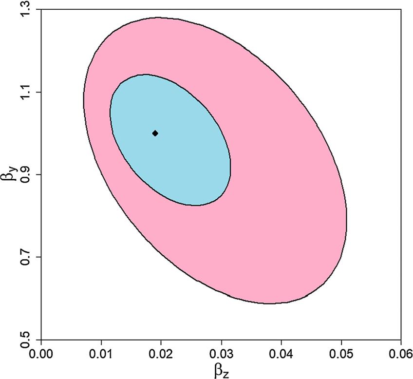
Fig. 1 portrays an example in which ρ1 = 0 and ρ2 satisfies:
q2
ρ2 = .
|σz |2
When St = η(Zt ) is restricted to be η1 (Zt − z̄), a given value of q imposes a restriction on η1
and, through equation (27), implicitly on (βy , βz ). Fig. 1 plots the q = .05 iso-entropy contour as
the boundary of a convex set for (βy , βz ).19
While Fig. 1 displays contours of time-invariant parameters with the same relative entropies
as the boundary of convex region, our restriction allows parameters (βy , βz ) to vary over time
provided that they remain within the plotted region. Indeed, we use (10) as a convenient way to
build a set of structured models. While we motivated this construction as one with time varying
parameters that lack probabilistic descriptions of how parameters vary, we may alternatively
view the set of structured models as inclusive of a restricted set of nonlinear specifications of the
conditional mean dynamics.
If we were to stop here and endow a max-min decision maker with the set of probabilities
determined by the set of martingales Mo , we could study max-min preferences associated with
19 This figure was constructed using the parameter values:
αy = .484 y
β = 1
αz = 0 z
β = .014
(σy ) = .477 0
(σz ) = .011 .025
taken from Hansen and Sargent (2020).
19You can also read