The Gardens2 algorithm - Repositorio INAOE
←
→
Page content transcription
If your browser does not render page correctly, please read the page content below
The Gardens2 algorithm

               Jonás Grande-Barreto
              Marı́a del Pilar Gómez-Gil

                             Manual

      Department of Computer Science
National Institute of Astrophysics Optics and
                 Electronics
             Tonantzintla, Puebla

                        c INAOE 2021
                          All rights reserved

  The authors hereby grants to INAOE permission to reproduce and to

                  distribute copies of this document.
1 Introduction
The Gardens2 algorithm [Grande-Barreto and Gómez-Gil, 2020] was developed to improve the
co-registration output of a generic brain atlas tissue templates to a specific brain target. As
a secondary task, the Gardens2 algorithm also can perform hard segmentation. The Gardens2
algorithm was implemented on MATLAB, and all the MRI (brain and atlas) inputs are in NII
format. Make sure that the proper packaging for handling NII files is in your MATLAB software.
Here1 is the link to download a package to manipulate NII files. The brain atlases were downloaded
from the McConnell Brain Imaging Center [Fonov et al., 2009, Fonov et al., 2011]. The link is here2 .
The 3D slicer software [Fedorov et al., 2012] required to perform the initial co-registration process.
Here is the link3 . It is recommended to use a field bias correction on MRI volume to improve
subsequent algorithms’ output. For the implementation described in this document, the N4ITK
MRI Bias correction algorithm was used (included in the 3D slicer software). For the algorithm
parameters, it is recommended to use a full width at half maximum of 0.20.
2 The Gardens2 algorithm
The Gardens2 algorithm requires five NII and one MAT input files. The NII files consist in
the brain MRI, brain mask, and three brain tissue templates named cerebrospinal fluid (csf), gray
matter (gm), and white matter (wm). The MAT file contains the feature representation of the brain
MRI volume. The brain MRI volume used for the implementation was taken from the Internet Brain
Segmentation Repository (IBSR) [IBSR, 2007]. The implementation of the Gardens2 algorithm is
divided into two parts, hard segmentation and partial maps. But first, it is necessary to perform
co-registration and feature extraction.
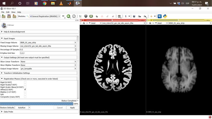
2.1 Atlas co-registration
It is necessary to carry out an initial co-registration process to align the scans of each of the tissue
templates with the brain MRI volume. The BRAINS algorithm [Johnson et al., 2007], included in
the 3D Slicer platform, was used to perform the initial co-registration process. This procedure
requires three inputs (tissue templates). For the implementation described by this manuscript
the files used were mni icbm152 csf tal nlin asym 09a, mni icbm152 gm tal nlin asym 09a, and
mni icbm152 wm tal nlin asym 09a. The outputs are csf template, gm template, and wm template.
the co-registration process is also required to generate the brain mask. For the implementation
described here, the file IBSR 01 ana brainmask (provided by the dataset) was co-registered to
generate the brain mask. Look the Figure 1 to learn the proper parameter settings.
2.2 Feature extraction
The feature representation procedure is composed by two functions cooc3d [Carl, 2021] and
GLCMFeatures [Brynolfsson, 2021]. Execute the script Feat represent.mat to compute feature rep-
resentation. This process requires the use of parallel computing, make sure you have this package
installed. For the implementation described by this manuscript the files required are brain mask
and IBSR 01 ana strip (mri volume).
1
https://la.mathworks.com/matlabcentral/fileexchange/8797-tools-for-nifti-and-analyze-image
2
http://www.bic.mni.mcgill.ca/ServicesAtlases/ICBM152NLin2009
3
https://download.slicer.org/
2Figure 1. Brain MRI scan.
2.3 Hard segmentation
This implementation performs a hard partition of the voxels for each scan of the brain MRI
volume. Open theGardens2 hard seg.mat script and execute lines 1 to 57 to initialize the internal
parameters of the Gardens2 algorithm. Load the required input files using the following lines
atlas_csf = load_nii ( ' Gardens2 pro \ csf_template . nii ') ;
atlas_gm = load_nii ( ' Gardens2 pro \ gm_template . nii ') ;
atlas_wm = load_nii ( ' Gardens2 pro \ wm_template . nii ') ;
GT = load_nii ( ' Gardens2 pro \ brain_gt . nii ') ;
brain_msk = load_nii ( ' Gardens2 pro \ brainmask . nii ') ;
load ( ' Gardens2 pro \ feats_Subject_x . mat ' , ' feat_all_ibsr ')
Transform the fuzzy labels of the brain tissue templates to a hard label format
[ Atlas_parcial , Atlas_crisp ] = Atlas_ref ( mri , atlas_csf , atlas_gm , atlas_wm ) ;
Next, it is necessary to calculate some indices to match the tissue templates’ information with
the feature representation
[ col , row , dip ] = size ( mri . img ) ;
midd = round (( rt (2) - rt (1) ) /2) + rt (1) ;
slix = midd - 20 : midd + 29;
point = rt (1) : rt (2) ;
scan_length = length ( slix ) ;
Inside the main for loop (for scan = 1 : scan length), the tissue templates’ information and the
feature representation are matched. The images are oriented in the axial plane. If the matching is
correct, for the first iteration, the image depicted in Figure 2 will show up.
3Figure 2. Brain MRI scan.
data = zeros ( row * col ,35) ;
sliceg = slix ( scan ) ;
xslice = find ( point == sliceg ) ;
Atlas_crisp_n = imrotate ( Atlas_crisp (: ,: , sliceg ) ,90) ;
Atlas_parcial_n = imrotate ( Atlas_parcial (: ,: , sliceg ) ,90) ;
mask = double ( imrotate ( round ( abs ( brain_msk . img (: ,: , sliceg ) ) ) ,90) ) ;
xs = find ( mask ) ;
data ( xs ,:) = feat_all_ibsr (1: length ( xs ) ,: , xslice ) ;
lnnan = isnan ( data ) ;
data ( lnnan ) = eps ;
ld = 16:35;
data (: , ld ) = [];
BI = reshape ( data (: ,13) ,row , col ) ;
aux = normalize ( data ( xs ,:) ) ;
data ( xs ,:) = aux ;
imshow ( BI ,[] , ' InitialMagnification ' , ' fit ')
In digital image processing, the over-segmentation is an undesired result. However, in the Gar-
dens2 pipeline, the over-segmentation is an intermediate output used to identify homogeneous
regions in the image. The following lines perform the over-segmentation using the watershed trans-
formation. The image depicted in Figure 3 will show up if the over-segmentation was successfully
executed.
[ J3 ,~] = imgradient ( BI , ' sobel ') ;
L = watershed ( J3 ) ; % Watershed transformation
LIO = logical ( L ) ; %
subregion = max ( L (:) ) ; % # de subregiones
subRs = zeros ( subregion , size ( data ,2) ) ;
for k =1: subregion
index = find ( L == k ) ;
subRs (k ,:) = mean ( data ( index ,:) ,1) ;
end
subRs (1 ,:) = [];
subregion = size ( subRs ,1) ;
La = double ( L ) ;
La = La - 1;
lnan = L == 1;
ln0 = L == 0;
La ( lnan ) = 0;
4La ( ln0 ) = 0;
g0 = LIO ==0;
AA = BI ; AA ( g0 ) = 0;
imshow ( AA ,[] , ' InitialMagnification ' , ' fit ')
The Gardens2 algorithm is machine learning-based; therefore, it requires the computation of
centroids for each tissue class to later perform the voxel clustering. The following lines execute
these procedures. If the code compiles correctly, the image depicted in Figure 4(a) will show.
% % Centroid computation
[ idx , Ci , tsamp ] = refsubRs ( subRs , LIO , La , data , Atlas_crisp_n ,...
subreg_cent , tissues ) ;
[ suger , Sub_inx , Cin_o , Gardened ] = suggestedsubregion ( subRs , percent_inclu , Ci ,...
Atlas_parcial_n , La , tissues , data ) ;
% % Clustering subregions
Dis_n = zeros ( subregion , tissues +2) ;
RN = 1 : subregion ;
Cin_old = Cin_o ;
for k = 1: subregion
while true
r = randi ([ min ( RN ) , max ( RN ) ]) ;
ri = find ( RN == r ) ;
if ~ isempty ( ri )
RN ( ri ) = [];
break
end
end
B = subRs (r ,:) ;
l2 = find ( La == r ) ;
A = Cin_old ;
Dis_n (r ,1: tissues ) = sum ( A .^2 - 2* A .* B ,2) ';
[~ , lr ] = min ( Dis_n (r ,1: tissues ) ) ;
Dis_n (r , end ) = lr ;
Sub_inx ( r ) = lr ;
Gardened ( l2 ) = lr ;
imshow ( Gardened ,[] , ' InitialMagnification ' , ' fit ')
end
Oversegmentation
Figure 3. Result of the watershed transformation for the Brain MRI scan.
5(a)
(b)
Figure 4. Hard segmentation result of the Gardens2 algorithm.
The watershed borders voxels are clustered using euclidean distance. The final result for the first
scan of the brain MRI volume is depicted in Figure 4(b). Repeat the process for the remaining
images of the volume.
% % Clustering of isolated voxels ( Watershed borders voxels )
isolated_vox = mask & ~ La ;
lf = find ( isolated_vox ) ;
A = Cin_o ;
for q = 1 : length ( lf )
B = data ( lf ( q ) ,:) ;
srd = sum ( A .^2 - 2* A .* B ,2) ;
[~ , srm ] = min ( srd ) ;
Gardened ( lf ( q ) ) = srm ;
end
imshow ( Gardened ,[] , ' InitialMagnification ' , ' fit ')
2.4 Partial tissue maps
This implementation performs an atlas adjustment for the tissue templates. Before starting, it
is necessary to execute theGardens2 hard seg.mat script; some parameters computed in that script
6are required for this part of the code. Open theGardens2 partial maps.mat script and execute the
lines 1 to 45 to load the required input scripts and set internal parameters of the algorithm. Partial
tissue maps are calculated using a novel fuzzy function composed by the Euclidean distance and a
regularization term. The centroids for each class are calculated with the following lines
% % Compute general centroids for the whole MRI volume
for qp = 1 : zli
c1 ( qp ,:) = CI (1 ,: , qp ) ;
c2 ( qp ,:) = CI (2 ,: , qp ) ;
c3 ( qp ,:) = CI (3 ,: , qp ) ;
end
K (1 ,:) = mean ( c1 ,1 , ' omitnan ') ;
K (2 ,:) = mean ( c2 ,1 , ' omitnan ') ;
K (3 ,:) = mean ( c3 ,1 , ' omitnan ') ;
The core of the code is the functionstepfcm2, which computes the tissue maps adjustment. This
function first computes the euclidean distance for the analyzed voxels
% % Euclidean distance
% Voxels to analyze
xs = find ( IM ) ;
dist = zeros ( size ( Ci1 , 1) , size ( aux , 1) ) ;
for k = 1: size ( Ci1 , 1)
dist (k , :) = sqrt ( sum ((( aux - ones ( size ( aux ,1) ,1) * Ci1 (k ,:) ) .^2) ,2) ) ;
end
The regularization process consists of adding a compensation factor, taken from the neighbor
voxels on the partial maps, to the estimated euclidean distance. The regularization factor is large
when the membership degree of neighboring voxels is large to tissue classes different from the
analyzed. Therefore, a voxel’s membership degree to a particular tissue class is large when the
euclidean distance and the membership degree of neighboring voxels to other tissue classes are low.
The following lines execute the outlined process
% % Regularization
dist3 = zeros ( size ( Ci1 , 1) , size ( aux , 1) ) ;
for k = 1 : size ( aux , 1)
[ xa , ya ] = ind2sub ([ row +(2* d3 ) , col +(2* d3 ) ] , xs ( k ) ) ;
x3 = xa ;
y3 = ya ;
Ia = ( tempA ( x3 - d3 : x3 + d3 , y3 - d3 : y3 + d3 ,:) ) ;
for q = 1 : tissues
g = ones (1 ,3) ;
g ( q ) = 0;
p2 = gamma * sum ( sum (( Ia .* w ) .^ expo ) ) ;
p2 = p2 (:) ;
p2 = g * p2 ;
dist3 (q , k ) = dist (q , k ) + p2 ;
end
end
tmp3 = dist3 .^( -2/( expo -1) ) ;
U_new3 = tmp3 ./( ones ( tissues , 1) * sum ( tmp3 ) ) ; %
U_new3 = round ( U_new3 ,2) ;
7Finally, the adjusted membership degrees of each tissue class are sorted to be displayed in image
format. If the code compiles correctly, the image depicted in Figure 5 will show.
% % Sorting and visualization
for qp = 1 : 3
temp4 = zeros ( row , col ) ;
temp4 ( xs ) = U_new3 ( qp ,:) ;
tempa (: ,: , qp ) = temp4 ;
end
csf_u (: ,: , scan ) = tempa (: ,: ,1) ;
gm_u (: ,: , scan ) = tempa (: ,: ,2) ;
wm_u (: ,: , scan ) = tempa (: ,: ,3) ;
subplot (2 ,2 ,1)
imshow ( BI ,[] , ' InitialMagnification ' , ' fit ')
title ( ' MRI ')
subplot (2 ,2 ,2)
imshow ( tempa (: ,: ,1) ,[] , ' InitialMagnification ' , ' fit ')
title ( ' CSF partial map ')
subplot (2 ,2 ,3)
imshow ( tempa (: ,: ,2) ,[] , ' InitialMagnification ' , ' fit ')
title ( ' GM partial map ')
subplot (2 ,2 ,4)
imshow ( tempa (: ,: ,3) ,[] , ' InitialMagnification ' , ' fit ')
title ( ' WM partial map ')
MRI CSF partial map
GM partial map WM partial map
Figure 5. Partial maps for the brain MRI scan.
8References
[Brynolfsson, 2021] Brynolfsson, P. (2021). Vectorized GLCM Texture features calculations. MAT-
LAB Central File Exchange.
[Carl, 2021] Carl (2021). 3D statistical texture algortihm. MATLAB Central File Exchange.
[Fedorov et al., 2012] Fedorov, A., Beichel, R., Kalpathy-Cramer, J., Finet, J., Fillion-Robin, J.-
C., Pujol, S., Bauer, C., Jennings, D., Fennessy, F., Sonka, M., et al. (2012). 3d slicer as an
image computing platform for the quantitative imaging network. Magnetic resonance imaging,
30(9):1323–1341.
[Fonov et al., 2011] Fonov, V., Evans, A. C., Botteron, K., Almli, C. R., McKinstry, R. C., Collins,
D. L., Group, B. D. C., et al. (2011). Unbiased average age-appropriate atlases for pediatric
studies. Neuroimage, 54(1):313–327.
[Fonov et al., 2009] Fonov, V. S., Evans, A. C., McKinstry, R. C., Almli, C., and Collins, D.
(2009). Unbiased nonlinear average age-appropriate brain templates from birth to adulthood.
NeuroImage, (47):S102.
[Grande-Barreto and Gómez-Gil, 2020] Grande-Barreto, J. and Gómez-Gil, P. (2020). Segmenta-
tion of mri brain scans using spatial constraints and 3d features. Medical & Biological Engineering
& Computing, 58(12):3101–3112.
[IBSR, 2007] IBSR (2007). Internet brain segmentation repository. Massachusetts General Hospital,
Center for Morphometric Analysis.
[Johnson et al., 2007] Johnson, H., Harris, G., Williams, K., et al. (2007). Brainsfit: mutual infor-
mation rigid registrations of whole-brain 3D images. Insight J, 57(1):1–10.
9You can also read