The Global Meteor Network - Methodology and First Results

MNRAS 000, 1–30 (2020) Preprint 2 August 2021 Compiled using MNRAS LATEX style file v3.0

 The Global Meteor Network - Methodology and First Results

 Denis Vida,1,2★ Damir Šegon3,4 , Peter S. Gural5 , Peter G. Brown1,2 , Mark J.M. McIntyre6 ,
 Tammo Jan Dijkema7 , Lovro Pavletić8 , Patrik Kukić9 , Michael J. Mazur1 ,
 Peter Eschman 10 , Paul Roggemans11 , Aleksandar Merlak12 and Dario Zubović4
 1 Department of Physics and Astronomy, University of Western Ontario, London, Ontario, N6A 3K7, Canada
 2 Institute for Earth and Space Exploration, University of Western Ontario, London, Ontario, N6A 5B8, Canada
 3 Astronomical Society Istra Pula, Park Monte Zaro 2, HR-52100 Pula, Croatia
 4 Višnjan Science and Education Center, Istarska 5, HR-51463 Višnjan, Croatia
arXiv:2107.12335v3 [astro-ph.EP] 29 Jul 2021

 5 Gural Software and Analysis LLC, Lovettsville, Virginia, USA
 6 Tackley Observatory, 40 Medcroft Road, Tackley, Oxfordshire OX5 3AH, UK
 7 ASTRON, Netherlands Institute for Radio Astronomy, Oude Hoogeveensedijk 4, 7991 PD Dwingeloo, The Netherlands
 8 Department of Physics, University of Rijeka, HR-51000 Rijeka, Croatia
 9 Faculty of Electrical Engineering and Computing, University of Zagreb, HR-10000 Zagreb, Croatia
 10 New Mexico Meteor Array, Albuquerque, New Mexico, USA
 11 Pijnboomstraat 25, 2800 Mechelen, Belgium
 12 Istrastream d.o.o, Hum, Croatia

 Accepted 2021 July 7. Received 2021 July 6; in original form 2021 January 26.

 ABSTRACT
 The Global Meteor Network (GMN) utilizes highly sensitive low-cost CMOS video cameras
 which run open-source meteor detection software on Raspberry Pi computers. Currently, over
 450 GMN cameras in 30 countries are deployed.
 The main goal of the network is to provide long-term characterization of the radiants,
 flux, and size distribution of annual meteor showers and outbursts in the optical meteor mass
 range. The rapid 24-hour publication cycle the orbital data will enhance the public situational
 awareness of the near-Earth meteoroid environment. The GMN also aims to increase the
 number of instrumentally observed meteorite falls and the transparency of data reduction
 methods.
 A novel astrometry calibration method is presented which allows decoupling of the camera
 pointing from the distortion, and is used for frequent pointing calibrations through the night.
 Using wide-field cameras (88° × 48°) with a limiting stellar magnitude of +6.0 ± 0.5 at 25
 frames per second, over 220,000 precise meteoroid orbits were collected since December 2018
 until June 2021.
 The median radiant precision of all computed trajectories is 0.47°, 0.32° for ∼ 20% of
 meteors which were observed from 4+ stations, a precision sufficient to measure physical
 dispersions of meteor showers. All non-daytime annual established meteor showers were
 observed during that time, including five outbursts. An analysis of a meteorite-dropping
 fireball is presented which showed visible wake, fragmentation details, and several discernible
 fragments. It had spatial trajectory fit errors of only ∼40 m, which translated into the estimated
 radiant and velocity errors of 3 arc minutes and tens of meters per second.
 Key words: meteors – meteoroids – comets

 1 INTRODUCTION distribution within streams can therefore provide unique insights
 into parent body physical properties and evolution (e.g. Egal et al.
 Measuring the activity and variability of meteor showers has been
 2020).
 a long term goal of meteor science. Meteor showers provide a
 direct link in many cases to known parent bodies (Vaubaillon et al. Recording meteor shower activity variations and physical char-
 2019). Characterization of the absolute flux, variability and particle acteristics such as radiants, particle size distributions and orbits is
 difficult. In particular, flux measurements require persistent, global
 observations and necessarily cannot be done from a single location.
 ★ E-mail: dvida@uwo.ca Some of the earliest success in near continuous, global monitoring

 © 2020 The Authors

2 D. Vida et al.
of meteor shower activity were performed in the 1980s by visual ob- expected to be optically observed. The number of actual meteorite
servers distributed across many longitudes during the 1988 Perseid recoveries will further be reduced due to inhospitable field terrain.
meteor shower (Roggemans 1989). An initiative aimed at addressing the problem of the small
 While visual records of meteor showers have been shown to be numbers of instrumentally recorded meteorite producing fireballs
valuable, they suffer some drawbacks. Visually, only the strongest is the Global Fireball Observatory (GFO) project (Devillepoix et al.
showers have reliable activity profiles as background contamina- 2020). This effort grew out of the regional Desert Fireball Network
tion becomes a problem (Rendtel et al. 2020). Moreover, visual (Howie et al. 2017). The GFO aims to rapidly expand the rate of
observations cannot be used to compute individual radiants, orbits meteorite recovery by covering 2% of the Earth’s surface by the
or examine ablation characteristics of shower meteors (begin/end early 2020s with modern high resolution DSLR cameras. When
height, deceleration, lightcurves) which may be used to infer phys- complete, the GFO expects to record ∼ 50 meteorite falls a year.
ical structure of meteoroids (Borovička et al. 2019). Optical instru- Here we describe the development and architecture of the
ments, however, can measure these quantities. Global Meteor Network (GMN), an analog to the GFO, but focused
 on fainter meteors. The broad goal of the GMN is to greatly expand
 Historically, optical networks have had a regional focus, often
 the atmospheric coverage of video networks to a global scale, per-
with the goal of recording meteorite producing fireballs (Halliday
 mitting continuous optical observations of meteors, using a fully
1971). The lower sensitivity and small number of stations on a
 open source software and data model. The intent is to make au-
global scale have, until recently, prevented such networks from be-
 tomated, reproducible detections and all associated measurements
coming a mainstay for monitoring meteor showers. Since the 1990s,
 of individual meteors immediately available for analysis by all in a
the advent of sensitive and inexpensive digital and video cameras
 fully transparent software pipeline.
has revolutionized optical meteor astronomy (Koten et al. 2019). As
a consequence, numerous dedicated regional video networks have Presently, most video meteor networks are either national or re-
been established (e.g. Weryk et al. 2007; SonotaCo 2009; Jenniskens gional, with some efforts to merge data sets from different networks
et al. 2011; Molau & Barentsen 2013; Vida et al. 2014). As digital (e.g. Kornos et al. 2014). Networks with the largest coverage consist
video cameras have become widely used in distributed meteor net- of amateur astronomers or citizen scientists hosting cameras at local
works they have also become widely adopted by many amateur and observatories or their private residences (e.g. Jenniskens et al. 2011;
professional observers. This is largely due to the commercial avail- Molau & Barentsen 2013). Additionally, complete data from these
ability of cheap, easy to use and highly sensitive low-light cameras. networks are often neither publicly available in near real-time nor
The most common model of data collection is to have one or more are the original data readily available for independent reductions
cameras connected to a computer running automated meteor detec- and quality checks. The Cameras for Allsky Meteor Surveillance
tion - the multi-station data is then sent to a central server where (CAMS) network is the closest to having a global presence, with
observations are paired and meteor trajectories computed. stations on all continents except Antarctica (Bruzzone et al. 2020).
 Most video networks also store data in mutually incompatible
 In the last decade, video meteor systems have matured to the
 formats, the data calibration procedures are not transparent or well
point where they have made substantial contributions in a number
 documented and data are reduced using proprietary software. Fur-
of areas. This includes the discovery of dozens of new established
 thermore, the data are usually published years after being collected.
meteor showers and hundreds of meteor shower candidates (Vida
 This leads to uncertainty in data quality and makes reproducib-
et al. 2013; Andreić et al. 2014; Jenniskens et al. 2016b; Jenniskens
 lity challenging. Finally, the lags in publication of the data negates
2017), measuring meteor shower flux (Molau & Barentsen 2014;
 its use for real-time near-Earth meteoroid environment situational
Ehlert & Erskine 2020), estimating population indices of meteor
 awareness. High quality data sets that do exist are usually composed
showers (Molau 2015), and recovery of meteorites produced by
 of manually calibrated and reduced data (e.g. Borovička et al. 2005;
bright fireballs (Borovička et al. 2015). Similar networks have also
 Campbell-Brown 2015), but manual labour is expensive, severely
been used to observe rare meteor shower outbursts and validate the
 limits the number of reduced meteors, and introduces subjective
existence of weak meteor showers (Holman & Jenniskens 2012;
 biases.
Šegon et al. 2014; Jenniskens et al. 2016a; Sato et al. 2017).
 Finally, most existing meteor network hardware is relatively
 While the foregoing networks have largely emerged out of expensive and specialized from an amateur astronomer perspective.
regional efforts, to achieve persistent global sky surveillance both The cost of deploying a single system is currently close to $1000
hemispheres and a wide range of longitudes must be instrumented. USD, including a camera and a computer. This is prohibitive for
This ensures that unique short-duration meteor shower outbursts are citizen scientists from low-income countries where sky coverage is
not missed due to timing (e.g. during the day for some observers) particularly desirable. Our goal is to lower the cost of entry into this
or as a result of poor local weather conditions. For example, no domain by a factor of 5 to 10 for a single-camera system.
published optical observations of the unexpected 2012 Draconid A major motivator for establishment of the Global Meteor Net-
meteor storm (ZHR ∼ 9000 at radar sizes) exist because the peak work (GMN) project is to build a distributed meteor network which
of activity occurred in darkness over central Asia where no meteor is treated as a fully automated decentralized science instrument. In
cameras were operating at the time (Ye et al. 2014). its final mature form, we envision GMN observing the night sky
 A similar challenge exists in trying to record meteorite- every night of the year from as many locations around the world
producing fireballs where the goal is to provide spatial context in as possible using citizen scientists as hosts. To achieve this goal,
the solar system for recovered samples. Annually, about 10 fireballs the installation cost and day-to-day operations must be accessible
drop at least 300 g of meteorites over an area of 0.5 million square to an average amateur astronomer. GMN data quality should mimic
kilometers, the size of a typical current regional network - e.g. Cali- as closely as possible high-precision manual reductions through
fornia, France, or Spain (Halliday et al. 1989; Bland et al. 1996). As implementation of frequent automated astrometric and photomet-
fireballs can only be well observed at night and 50% of the planet is ric recalibrations, and by applying rigorous filtering of the final
covered by clouds at any given time (global average; Stubenrauch data products. All filtering, calibrations and analysis procedures are
et al. 2013), only two to three such meteorite dropping fireballs are based on an open source software architecture and are to be docu-

 MNRAS 000, 1–30 (2020)

Global Meteor Network 3
mented. Sufficient Level 0 data products are retained so anyone can
fully reprocess detections either with their own software or using
manual reduction tools provided with the GMN software suite.
 The main science goals of the Global Meteor Network are:

 (i) To provide the public with near real-time awareness of the
near-Earth meteoroid environment in the optical meteoroid mass
range (mm-sizes and larger) by publishing orbits of meteors within
24 hours of their observation. A yearly average of 1000 orbits/day
are set as an initial operational goal, bringing the GMN close to
the orbit numbers observed by meteor radars and therefore permit-
ting automated statistical detections of meteor showers (Jones et al.
2005; Brown et al. 2010).
 (ii) To create a continuous record of annual meteor showers and
meteor shower outbursts for future research. In particular, the flux, Figure 1. A full night of stacked images showing maximum pixel values
mass indices, and orbits of shower meteors will be computed with during meteor detections. Over 300 meteors are visible in this stack from
each trajectory and the orbit will have an associated covariance Oct 9, 2018 during the Draconid outburst as imaged by the HR0010 camera
matrix. in Croatia (color-inverted). The slanted dashed lines are bright stars which
 (iii) To provide high-resolution observations of meteorite- drift through the field over the course of the night relative to the fixed camera.
producing fireballs with the aim of increasing the number of mete- The field of view is 88° × 48°.
orites with known orbits (only ∼ 40 published orbits up until mid-
20211 ) to improve number statistics to constrain meteorite source (Vida et al. 2019). As an example, Figure 1 shows a co-added im-
regions in the Solar System. An additional by-product of GMN age of the 2018 Draconid outburst (Egal et al. 2018) observed by a
high-quality observations is the prospect of recording the formation GMN camera in Croatia (Vida et al. 2018a).
of fireball wake and details of fragmentation which can be used Recognizing that amateur astronomers are an invaluable re-
to estimate the physical properties of large meteoroids (Borovička source as they can offer their time and enthusiasm to operate and
et al. 2020; Shrbený et al. 2020). invest a small amount of money towards a meteor camera, the GMN
 is built around amateur participation. In this way, GMN has out-
 sourced funding, maintenance, and deployment to private parties.
1.1 Concept of Operations The GMN project opened the development of software to contrib-
 utors from the general public, but still retains control over final
The current model used by most professional video meteor networks software changes, ensuring a stable, common code base.
is to have a team which applies for funding, builds and distributes As many amateur astronomers tend to install meteor cameras
meteor camera systems, and handles long-term maintenance of the close to their residence, and due to the modular design of the system,
network, with station operators in passive support roles. In contrast, maintenance is simple. No component of the system costs more
the Global Meteor Network philosophy is to reduce the time and than $50 USD and most parts can be sourced locally. The network
money spent by scientists on building hardware and on day-to-day is loosely organized on the global scale and divided into national
operations. GMN provides a blueprint and a list of parts for a me- or regional sub-networks. Some stations consist of lone camera
teor camera so anyone can build one. Additionally, building has operators who manage several cameras and choose not to closely
been outsourced to a private company which offers compatible plug interact with local networks.
and play systems for purchase at low cost. Interested individuals Operationally, once a camera is deployed, the station operator
then build and deploy the systems, which are then automatically contacts the network coordinator who assigns a unique station code.
connected to the main GMN server which collects, processes, cor- The code consists of an ISO-2 country code followed by four al-
relates and quickly publishes all daily GMN detections. phanumeric characters, e.g. US001A. Next, the network coordinator
 In the most common configuration, the imaging part of a GMN creates an astrometric calibration plate which the operator uploads
system consists of a low-light Internet Protocol (IP) camera board to their station. After the network coordinator inspects the quality
(∼$30 USD), a 3.6 mm f/0.95 CCTV lens (∼$10 USD), and an of the data and ensures that the automated recalibration procedure
aluminium housing (∼$20 USD). The most expensive part of a me- works well (described in detail in Section 2.5), the camera is added
teor station, the personal computer, is replaced by a Raspberry Pi into the automated trajectory estimation pipeline. Finally, meteor
(RPi) single-board computer (∼$35 USD) in the GMN. Together observations from multiple stations are automatically correlated.
with other accessories, the total cost of parts for one meteor station Associated meteor trajectories and additional metadata are typi-
is around $200 USD (circa 2021). The stations run Raspberry Pi cally available on the Global Meteor Network’s website3 within 24
Meteor Station (RMS) open-source software2 that is simple to con- hours of when the meteor was observed.
figure and requires little to no user attention on a day-to-day basis.
This hardware configuration achieves a limiting stellar magnitude
of +6 ± 0.5 and 10-100 meteor detections on a typical night. This 1.2 Overview of current status
rate may surpass thousands during the peak of the Geminid shower
 The first GMN systems were deployed in the spring of 2018. Since
 then, the network has experienced a rapid expansion, with the num-
 ber of cameras as of mid-2021 in excess of 450 in 30 countries. Fig-
1 List of meteorite orbits: http://www.meteoriteorbits.info/
2 RMS software library: https://github.com/
CroatianMeteorNetwork/RMS 3 Global Meteor Network data: globalmeteornetwork.org/data/

MNRAS 000, 1–30 (2020)

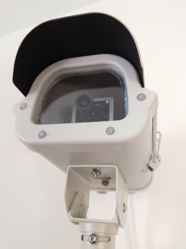
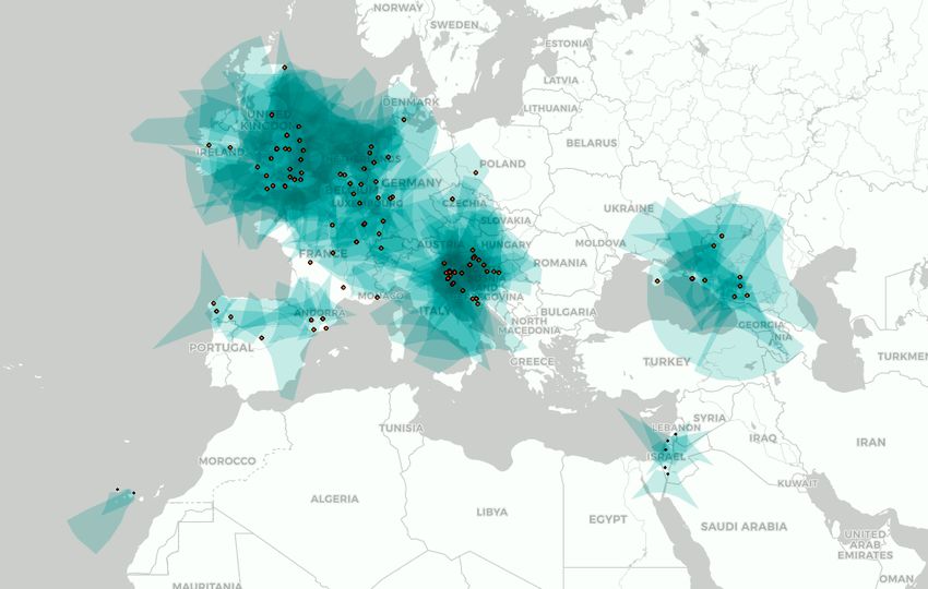
4 D. Vida et al.
 GMN, with a particular focus on calibration methods. We also out-
 line what we have found empirically to be best practices for com-
 puting reliable meteor trajectories from video observations, both
 manually and in an automated way. In Section 3 we present some
 first preliminary scientific results. In this section we also discuss
 the data accuracy, the observed orbital and magnitude distribution,
 and observations of established meteor showers and outbursts that
 occurred in 2019 and 2020. Finally, we highlight GMN’s capabil-
 ity for recording fireballs by presenting an analysis of one recent
 meteorite-dropping fireball.

 2 METHODS
 2.1 Hardware Evolution
 Zubović et al. (2015) were the first to demonstrate that Raspberry Pi
 2 single-board computers6 are powerful enough to replace personal
 computers for video meteor data capture and automated processing.
 Their prototype meteor camera system had a total cost of only
 $150 USD (in parts), an order of magnitude less than any other
 video meteor systems deployed at the time. As there was no freely
 available software which would run on Linux operating systems,
 Vida et al. (2016) developed novel open-source meteor, fireball,
 and star detection algorithms.
 Initial tests with this system were performed using analog Sony
 ICX-673 Charge Coupled Device (CCD) cameras and an EasyCap
Figure 2. Field of view coverage (light blue) projected to a height of 100 km frame grabber (Vida et al. 2018b) which produced a standard defi-
for currently operational GMN cameras (dots) in Europe (top) and North nition (720 × 576) interlaced video at 25 frames per second (FPS).
America (bottom). Taken from the meteor map website5 .
 However, this system architecture was potentially weak in terms of
 long term support and replacement as Sony ceased production of
 CCD sensors in 2015. Such sensors were ubiquitously used in video
ure 2 shows fields of view of currently operational GMN cameras
 meteor work and in 2015 there were no comparable complementary
in Europe and North America (a few cameras in Brazil, Australia,
 metal–oxide–semiconductor (CMOS) imaging chip alternatives.
and New Zealand are not shown).
 In 2017, Hankey & Perlerin (2018) reported first results with
 The data collected by the GMN in this early period has been
 a low-cost and highly sensitive Sony IMX290 CMOS sensor em-
used in several studies, demonstrating the versatility of GMN data.
 bedded in a commercial of the shelf (COTS) IP camera providing
Moorhead et al. (2020) presented a new method of measuring the
 high definition (1920 × 1080) video at 25 FPS. These digital cam-
radiant dispersion of meteor showers, applying the technique to the
 eras send the video stream via an Ethernet connection and support
Orionids and the Perseids using GMN data. The analysis will be
 Power-over-Ethernet (PoE), simplifying the installation procedure.
expanded in a future paper. The measured dispersions were tighter
 This simplifies connecting multiple cameras into a single PoE net-
than reported by other authors in the past and larger than the inter-
 work switch while running only one cable to each camera. One
nally estimated measurement accuracy based on the Monte Carlo
 downside of these new COTS cameras is that they compress the
procedure (Vida et al. 2020a), suggesting that the true, physical
 video stream using the H.264 compression standard, which is lossy
radiant dispersion was observed for the first time.
 and requires additional computing to be decompressed introducing
 Vida (2020) compared high-precision manual radiant mea-
 additional computational overhead.
surements of the Orionids done using the Canadian Automated
 In late 2017, a more powerful RPi 3 became available which
Meteor Observatory’s mirror tracking system (Weryk et al. 2013;
 Vida et al. (2018b) tested using a newer IMX291 based COTS
Vida et al. 2021) with GMN’s automated measurements and found
 CMOS IP camera paired with a 4 mm f/1.2 lens. This combination
good agreement between the two datasets. Roggemans et al. (2020a)
 produced a field of view (FOV) of around 90° × 45°. They demon-
used GMN observations of the enhanced activity of the h Virginid
 strated that such a setup can achieve a limiting stellar magnitude
meteor shower in 2020 to compute the mean orbit of the shower.
 of around +5.5 at 25 FPS in light-polluted city conditions. The
In that study, the GMN contributed the most observed trajectories
 IMX291 has a full HD (1920 × 1080 px at 25 FPS) 1/2.8" sensor
and the GMN mean orbit was in agreement with orbits reported
 with a pixel pitch of 2.9 µm and a quantum efficiency of ∼ 70%7 .
by other networks. Finally, Egal et al. (2020) performed dynam-
 Vida et al. (2018b) also showed that good photometric measure-
ical simulations of the Orionids and the -Aquariids, and shown
 ments can be performed using these CMOS sensors and that there
that the radiants observed by the GMN were a good match to their
 was a noticeable increase in sensitivity compared to previous CCD-
simulations.
 based cameras used for meteor observations. A major advantage
 We have organized this paper describing the GMN as follows.
 of the Raspberry Pi is that it has a powerful Graphical Processing
In Section 2 we summarize the hardware and software used by the

 6 Raspberry Pi foundation: https://www.raspberrypi.org/
5 Meteor map website: https://tammojan.github.io/meteormap/ 7 IMX291 datasheet, available from the manufacturer

 MNRAS 000, 1–30 (2020)

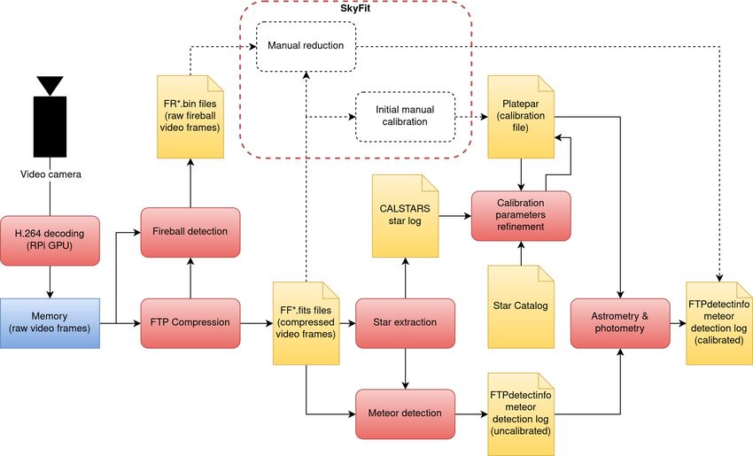
Global Meteor Network 5
Unit (GPU) which supports hardware H.264 decoding. This reduces
CPU overhead, although the resolution needs to be down-sampled
to 1280 × 720 px to ensure real-time processing. In addition to the
IMX291, cameras based on IMX307 and IMX385 were success-
fully tested and are in regular use, albeit in smaller numbers. We
also note that the RMS software supports any camera that can be
opened as a video device in the operating system.
 In contrast to analog CCD cameras, which provide interleaved
video signals, the IMX291 has a rolling shutter. In analog interleaved
video every other row is read out at the same FPS but offset in
time by half the FPS rate. This half frame spatial resolution is
termed a field. Therefore the fields per second rate is twice the
frames per second rate. For an IMX291 rolling shutter the sensor
continuously reads out video frames from the top of the frame to
the bottom such that the top and the bottom of video frames are
not phase synchronised. If meteor positions are measured using
such video, Kukić et al. (2018) have shown that the rolling shutter
effect introduces an angular velocity bias of up to several percent
for fast meteors observed using moderate field of view systems.
They developed a simple time correction which mitigates this effect
which is implemented within the GMN software library.
 Figure 3 shows a typical Global Meteor Network camera and
enclosure (circa mid-2021) while Figure 4 depicts a common in-
stallation arrangement. As of mid-2021, Raspberry Pi 3 and 4 are
the most commonly used boards. The Raspberry Pi is kept inside a
building because it would overheat during the summer if kept in the
camera housing, and there is a risk of water damage if the housing
is not completely waterproofed.
 The Raspberry Pis are equipped with an external real-time
clock module which keeps the correct time if it reboots. The time
is synchronized using the Network Time Protocol (NTP) protocol,
which is able to keep the correct time within at least one second. Figure 3. An assembled GMN camera system. The housing contains the
 lens and the sensor board (fan and heater optional).
Video frames are first encoded on the camera board, travel as trans-
mission control protocol (TCP) packets via Ethernet, and are finally
decoded on the Pi’s GPU. As a result, there is a fixed delay from
capture to recording of ∼2.2 s which is taken into account during
the trajectory estimation procedure.
 The GMN standard cameras typically use three types of lenses
with varying fields of views (see Table 1). A FOV comparison is
shown in Figure 5. The 3.6 mm f/0.95 lens affords a field of view
of 88° × 48° and is mostly used in dark locations. The 8 mm f/0.9
lens is used in heavily light polluted areas and has a field of view
of 40° × 22°. Finally, the 16 mm f/1.0 lens is useful for measuring
very precise meteor trajectories (astrometric precision of ∼ 0.1 arc
minutes) and has a FOV of 20°×11°. A dedicated network of twenty
three 16 mm systems is deployed in western Croatia.

2.2 Data acquisition and meteor detection
Figure 6 is a flowchart of the RMS data capture and calibration
pipeline. More details can be found in Vida et al. (2016, 2018b).
 The software automatically schedules data acquisition to be-
gin each night. This starts 30 minutes before and ends 30 minutes Figure 4. Diagram showing an installation of a GMN system. The Raspberry
after the local astronomical dusk and dawn, respectively. Video Pi is not kept inside the camera housing but inside the building to shield it
frames are compressed using the Four-frame Temporal Pixel (FTP) from the elements. The PoE cable may be tens of meters long and carries
 both the power and the digital video signal.
compression (Gural 2011), and stored to disk. A real-time fireball
detector stores raw frames of bright fireballs for posterior use.
 Stars and faint meteors are detected using a separate dedicated
detector, and the astrometry and photometry calibration is auto-
matically performed for each potential meteor detection. The end
product of this process is a list of meteor detections, with every
detection consisting of a set of time, position, and magnitude of

MNRAS 000, 1–30 (2020)

6 D. Vida et al.

Table 1. Comparison of lens fields of view and limiting stellar magnitudes with the IMX291 1/2.9" sensor. An image resolution of 1280 × 720 pixels is assumed.
Most of these lenses can be purchased for $10 - $20 USD.
 Focal length f-number FOV Stellar limiting magnitude Pixel scale (arcmin/px)
 3.6 mm f/0.95 88° × 48° +6.5 (ideal), +5.5 (city) 4.1
 6 mm f/0.95 53° × 30° +7.0 (ideal), +6.0 (city) 2.5
 8 mm f/0.9 40° × 22° +7.5 (ideal), +6.5 (city) 1.9
 16 mm f/1.0 20° × 11° +8.0 (ideal), +7.0 (city) 0.94
 25 mm f/1.2 13° × 7° +10.0 0.60

Figure 5. A comparison of the fields of view of lenses used by the GMN (color-inverted). The 16 mm lens provides a 4x better astrometric precision than the
3.6 mm lens, but it only covers ∼ 5% of that lens’ field of view.

the meteor on every video frame. The very first calibration file is approximation of the original video, the index of the video frame
created manually and then automatically updated thereafter numer- with the brightest pixel value is stored in the maximum frame index
ous times every night. Manual reduction of events of interest may image. Note that the number of frames in the block is chosen to
be performed if desired. The software automatically manages disk correspond to the number of discrete image levels in an 8-bit image
space, and the data is stored using a first-in, first-out approach where (28 = 256), so the index can be stored as an image level. If multiple
the oldest data is deleted to make room for the newest. frames have the same maximum value, the frame index is chosen
 The storage memory limitations of the Raspberry Pi are due to with a random number threshold dependent on how many times the
its use of micro-SD cards, which are currently limited to between 64 value is repeated.
to 256 GB at modest cost points. As a result, full raw video frames Inset b) in Figure 7 shows the gradient of the increasing bright-
(∼ 600 GB for an 8 hour night) are generally not stored to disk. To ness/index with the progression of the fireball towards the bottom
address this issue, the RMS software employs the FTP compression of the image. The average and standard deviation images, shown
method which provides a 64:1 compression ratio. This algorithm as insets c) and d), have the top four maximum values removed
takes a block of 256 raw video frames and compresses them into to mitigate the influence of bright fireballs on the estimate of the
four images which are saved into one Four Frame (FF) file in the background. This works well for fainter meteors, but as can be seen
Flexible Image Transport System (FITS) format, consisting of the in this case of a bright and slow-moving fireball which lasted over
maximum pixel, maximum pixel frame index, average pixel, and 120 frames, the standard deviation is contaminated by the meteor.
standard deviation image, each on an independent per pixel basis. The average and standard deviation frames are used by the
 In Figure 7 an example of each of these frames is shown. The meteor detection algorithm to determine which parts of the image
maximum pixel image only stores the maximum value of every contain a meteor by simply checking if the maximum value is a
pixel in the block of 256 frames, as shown in inset a). To preserve certain number of standard deviation above the mean. Finally, inset
the temporal information which allows reconstruction of a close e) shows co-added reconstructed video frames (every tenth) of the

 MNRAS 000, 1–30 (2020)

Global Meteor Network 7

Figure 6. A schematic of the RMS data flow and automated calibration procedure. Solid lines denote automated steps, while dashed lines indicate manual
steps. Red rectangles identify algorithms, and yellow rectangles represent data files.

fireball using the compressed frames. This reconstruction approach clear skies, 50-200 stars are usually detected on every FF image,
works well for faint meteors and the fainter parts of fireballs, but depending on the stellar limiting magnitude.
it creates artifacts for the brighter parts of fireballs simply because
it can only store one frame index for one brightest value. This
 If a minimum of 20 stars are visible, indicating that the skies
limitation was the reason a dedicated real-time fireball detector was
 are at least partially clear, a dedicated faint meteor detector is run
developed (Vida et al. 2016) which stores raw frames of fireballs
 on the FF file. This algorithm attempts to detect very faint meteors
while they are still available in memory and runs prior to the FTP
 and it requires more time to run than the fast fireball detector. In
compression. These raw frames can also be later used for manual
 summary, segments of 64 frames which are reconstructed from the
data reduction (e.g. see Figure 15).
 FF files and thresholded using a user-configurable simple image
 The star and meteor detection algorithms are run in parallel to
 operation max > avg + 1 + 1 , where values of 1 = 3.5 and
data acquisition. They asynchronously load the compressed FF files
 1 = 12 are most commonly used for IMX291 IP cameras. Next,
from a queue and may continue to run after the capture ends for
 a set of image morphological operators (clean, bridge, close, thin,
the night if processing has not been completed. The data process-
 clean; see Dougherty & Lotufo 2003) reduce potential meteors into
ing typically lasts no more than a few hours after the end of data
 thin lines while suppressing all background noise. A kernel-based
collection.
 Hough transform (Fernandes & Oliveira 2008) is applied to find
 The star extractor algorithm detects stars by finding local max-
 lines of pixels which may be meteor trails in the image, and line
ima on the average pixel image and attempts to fit a 2D Gaussian
 candidates are fed into a 3D line segment finding algorithm (where
point spread function (PSF) to them. The value of the Gaussian is
 dimensions are X, Y, and frame number) to check for temporal
limited to the saturation point (255 for 8-bit sensors), making it a
 propagation (Vida et al. 2016).
flat-topped distribution for bright stars that saturate the sensor. In
this way, a reliable fit and a rough estimate of the stars unsaturated
brightness is obtained. Star candidates which are not round (the If the detection covers at least 4 consecutive video frames and
smallest ratio between X and Y standard deviations is less than 0.5), has an angular velocity within the range of 2-51 ° s−1 (expected
or too large (2 > 5px), and for which the minimization procedure meteor range; Gural 1999), centroids and sums of pixel intensity
does not quickly converge are rejected. This method is found to be for every frame are computed within a ∼ 30 px wide rectangular
robust and also provides an estimate of the variation of the PSF segment with a length which varies with the angular velocity such
across the field of view. Generally, if the 3.6 mm lenses are well that it encompasses the whole meteor on every frame. Finally, the
mounted and focused, the PSF is constant across the whole field of rolling shutter correction is applied if necessary. For more algorith-
view with a full width at half maximum (FWHM) of ∼ 3 px. Given mic details, see Vida et al. (2016).

MNRAS 000, 1–30 (2020)

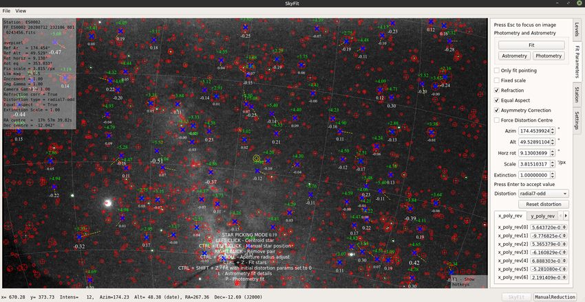
8 D. Vida et al.

Figure 7. FTP compressed images stored in an FF file of a fireball observed on January 22, 2020 over Southwestern Ontario. a) Maximum pixel image, b)
Maximum frame index image, c) Average image showing the background stars, d) Standard deviation image, e) Co-added every tenth reconstructed video
frame.

2.3 Astrometric and photometric calibration 256 frame average. Most commonly, the GAIA DR2 star catalog
 (Gaia Collaboration et al. 2018) is used, although others such as the
To produce useful astrometry and photometry for analysis of meteor Sky2000 and BSC5 are supported as well (see Appendix B). The
measurements, transformations of the pixel detections and intensi- resulting meteor measurements are reported in the J2000 epoch, to
ties from the focal plane to celestial coordinates and calibrated be consistent with the star catalog.
intensities on the sky must be performed.
 The transformation between image (x,y) coordinates and ce-
lestial coordinates ( , or equivalent) is performed using an astro-
metric plate. The GMN employs a simple plane projection approach
(Smart et al. 1977) which uses a novel radial distortion model with
odd terms up to the ninth order to construct an astrometric plate.
This approach can compensate for lens asymmetry and non-square 2.3.1 IMX291 spectral sensitivity
pixels using a total of only nine coefficients. Alternatively, a third The GAIA G band (not to be confused with the green filter) has a
order polynomial in (x,y) together with radial terms can be used. broad spectral sensitivity, with the transmissivity sharply rising at
This approach results in an astrometric plate with 12 distortion co- 400 nm and falling off at 900-1000 nm (Weiler 2018). This range
efficients per image axis (Vida et al. 2018b). A detailed description roughly matches the sensitivity of the IMX291 sensor with the IR
of the method is given in Appendix A. filter removed (Figure 9) and we use the G-band as a proxy for the
 The camera pointing (corresponding to the centre of the op- spectral system of the IMX291 chip.
tical axis) is defined in equatorial coordinates at a reference time However, the IMX291 sensors have a Bayer RGB filter and as
using four affine transform parameters: right ascension, declination, the cameras are operated in the black and white mode, the camera
position angle of the Y image axis, and plate scale. If the radial dis- computes the pixel intensity luma value as = 0.299 + 0.587 +
tortion is used, one polynomial describes the forward, and one the 0.114 (Burger & Burge 2010) (black line in Figure 9). Assuming
reverse mapping. If the polynomial distortion is used, four sets of no significant influence from the front glass or the lens (which are
polynomials describe the distortion - two sets for forward mapping unknown to us for these low-cost products), we can approximate the
(image to sky) and a second pair of sets for reverse mapping (sky to spectral sensitivity using a combination of Johnson-Cousins filters
image), one set for every image axis X and Y. (Jenniskens et al. 2011) as 0.15 + 0.30 + 0.25 + 0.30 (gray line
 When a new camera pointing is made, an initial astrometric in Figure 9). Nevertheless, we use the GAIA catalog as the spectra
calibration is preformed manually using the SkyFit program (based of meteors are essentially unknown and not all stars in the Sky2000
on a previous version from Vida & Novoselnik 2010) provided in catalog have BVRI values.
the RMS library. SkyFit allows calibrating and manually reducing Faster meteors radiate ∼ 20% more in the near infra-red
RMS format image files, as well as the Global Fireball Observatory (>700 nm) than slower meteors due to stronger atmospheric lines
(Howie et al. 2017) and FRIPON images (Colas et al. 2020), or (Šegon et al. 2018). Compared to previous Sony CCD sensors (e.g.
any media format supported by the OpenCV library (e.g. png, jpg, Jenniskens et al. 2011), the IMX291 sensors have a second peak of
avi, mp4; Bradski 2000). Figure 8 shows the SkyFit graphical user sensitivity at around 850 nm, which may be beneficial for detecting
interface. If the RMS data is used, the calibration is done on the faster meteors relative to earlier CCDs.

 MNRAS 000, 1–30 (2020)

Global Meteor Network 9

Figure 8. An example of the SkyFit graphical user interface with an overlaid equatorial grid showing a manual astrometric plate produced for a camera at
Roque de Los Muchacos, La Palma, Spain (the MAGIC telescope is visible in the bottom of the FOV). The effective stellar limiting magnitude of this 256
frame average is +6.7 . The red markers are catalog stars and their size indicates their magnitude (bigger means brighter). Blue markers indicate paired stars.
The yellow lines indicate the absolute value (times 100) and the direction of astrometric fit residuals. The green numbers are catalogue stellar magnitudes while
the white numbers below each star are the photometric residual per star for the given fit. The side bar at the right gives the details of the fit, and the status bar
at the bottom indicates the coordinates under the mouse cursor (currently pointing just below the middle of the image, as indicated by a yellow annulus).

 catalog stars. Clicking on a star produces a centroid and a sum of
 background-subtracted pixel intensities within an annulus of ad-
 justable size. If less than 12 stars are paired, only the four affine
 parameters are fit, which is useful if a user only wants to readjust
 the pointing and the distortion is already known. For the initial fit
 however, at least 40 stars are paired across the whole field of view
 to ensure a robust estimate of the distortion coefficients. We de-
 scribe the minimization procedure in detail in Appendix A1. The fit
 residuals for 3.6 mm lenses and 1280 × 720 resolution (plate scale
 of ∼ 4 ’/px) is usually around 0.2 pixels and 0.8 arcmin when the
 radial distortion model is used, although this may vary depending
 on the image quality. Some manual refinement is usually needed
 to achieve a precise astrometric fit: centroids for stars with high fit
 residuals are redone with a different spatial aperture, and picks are
 manually forced to a particular position if the star is not isolated.
 The photometric fit is performed taking system vignetting and
 atmospheric extinction into account. The procedure is described in
 detail in Appendix B. The fit is initially performed on the same
Figure 9. Top: Comparison between the GAIA G spectral passband and set of stars selected for astrometry, but some manual refinement
individual color filters of the IMX291 sensor. Bottom: IMX291 luma spectral is usually needed during which stars with high fit residuals are
sensitivity (after conversion to black and white) compared to the closest fitted removed (e.g. stars in clouds or haze), and some new stars are
Johnson-Cousins equivalent.
 added. An average photometric fit error for the zero-point (intercept)
 of ±0.15 magnitudes is usually achieved for the typical GMN setup.

2.3.2 Manual calibration procedure
 2.4 Calibration Examples
To create an initial astrometric plate, the user first manually de-
fines a rough pointing direction and the plate scale. There is also an For the purpose of illustrating the type of calibration that was used to
option to query astrometry.net (Lang et al. 2010) for an initial produce the results presented in this paper, Figure 10 shows details
astrometric solution. Then, the user manually pairs image stars to of the astrometric and photometric residuals done for a typical GMN

MNRAS 000, 1–30 (2020)

10 D. Vida et al.
station (shown in Figure 8). The astrometric fit was done using the the radius ensures that a rough match is obtained at first, and later
novel radial distortion model (with odd terms up to the 7th order) any false matches (e.g. binary stars) are excluded from the fit. A
which was adopted by the GMN in late 2020. The average image maximum median distance of = 0.33px is mandated. If the value
and angular fit residuals are 0.19 px and 0.78 arc minutes and show is higher even after recalibration, the procedure is considered to
no trends, which is what is expected for a "good" astrometric fit have failed. Figure 12 shows an automated recalibration on one FF
free of systematic errors. Prior to the development of the novel file while Figure 13 shows the pointing drift over the course of a
radial method in late 2020, most systems were calibrated using the night. Shifts of up to 10 arc minutes are often observed.
polynomial method (see Appendix A3). Using the same data set as If the initial shift is larger than 10 pixels and no stars are
above, the method produced average image and angular fit residuals matched, the phase correlation image alignment method based on
of 0.19 px and 1.27 arc minutes, respectively. Minor trends in the the Fourier transform (Reddy & Chatterji 1996) is used to estimate
residuals could have been seen. the translation, rotation, and scale from the initial pointing.
 Because the sensor is 8-bit, the effective dynamic range for this In this approach, a synthetic image is created with a black back-
camera is from magnitude +7.0 to +1.0 . For objects brighter ground and white points placed where detected stars are located.
than +1.0 the sensor will start to saturate. The photometric er- This is then fed into the algorithm, together with a synthetic image
ror in the zero-point fit is ±0.13 magnitudes, when vignetting and generated using the predicted positions of catalog stars. Using a
extinction are taken into account (see Appendix B). We attempted fast Fourier transform and image representation in log-polar form,
to perform a saturation correction using the numerical simulation a cross correlation between the images is performed. This becomes
method of Kikwaya et al. (2010), but it appears that the non-linearity simple multiplication in the Fourier space and can be performed at
of CMOS sensors close to saturation and the H.264 compression low computational cost. The method produces values of translation,
prevent the successful application of this approach; thus we do not rotation, and scale that need to be applied for the two input images
apply any saturation correction to our data. to match. In practice, this method reliably works for shifts of up to
 SkyFit can also fit astrometric plates using radial distortion 1/4 of the total image and virtually any rotation.
models for high-resolution all-sky images, such as those produced At the same cadence as the astrometric recalibration (i.e. at
by the Global Fireball Observatory system (Devillepoix et al. 2020). the time of every detected meteor), the photometric offset is also
Figure 11 shows the calibration residuals when SkyFit is applied recalibrated. It uses the same set of paired stars as used for the astro-
to one of these cameras. An average angular precision of 0.5 arc metric recalibration, while keeping the vignetting coefficient fixed.
minutes can be achieved, limited mainly by the deformation of the Frequent photometric recalibration is necessary because the sky
PSF at the edges of the field of view. The photometric fit errors are transparency may change rapidly due to humidity, clouds, increas-
on the order of ±0.1 magnitudes. See Appendix A6 for a detailed ing sky glow with the rising Moon, varying aerosol concentration,
performance comparison between different methods of astrometry etc. Figure 14 shows an example of how the photometric offset varies
calibrations on various types of cameras. during the course of one night. In this case the offset (zero-point)
 dips as the Moon enters the field of view. Differences throughout
 the night of more than one magnitude are commonly observed when
2.5 Automated recalibration the full Moon is close to the field of view.
During early operation of GMN, it was discovered that astrometric
calibrations done on images several hours apart were often shifted by
 2.6 Manual data reduction
several arc minutes. By inspecting the actual and predicted positions
of stars, a gradual drift in pointing was noticed. We believe this is The automated RMS meteor detector produces centroids and mag-
caused by thermal expansion of the camera metal housing, mounting nitude measurements for fainter meteors, but the separate fireball
bracket and/or the platform or building the camera is attached to. detector only stores raw frames for bright events. Due to the complex
 To mitigate this effect, we implemented an automated recali- morphology of fireballs (which often show long wakes, fragmenta-
bration routine for the camera pointing which is performed on every tion, and flares which may saturate a large image area), fireballs are
image with a meteor detection. Because the camera pointing in our manually reduced using SkyFit.
astrometric method is independent of the distortion, and we assume When performing fireball reduction in SkyFit, the astromet-
that the distortion should remain unchanged (as it depends only ric plate is manually re-fit using as many as possible stars in the
on the optics, which is stable), only the affine parameters (refer- vicinity of the fireball. Figure 15 shows an example of how manual
ence right ascension, declination, rotation, and scale) are adjusted astrometric and photometric picks are done on every frame. For the
in this process. Although in theory the scale should remain fixed, initial frames, where a fireball often does not saturate, centroiding
in practice we found slight but visible changes which need to be can be used to make precise picks, and the magnitude can be mea-
compensated for. sured by manually coloring the pixels which the user decides belong
 During the recalibration procedure, the catalog stars and stars to the meteor.
detected on the image are paired using progressively smaller match As the fireball penetrates deeper and develops a wake, the
radii, from 10 to 0.5 pixels. The pointing direction is found by min- picking becomes more difficult and sometimes has to be manually
imizing the match cost function for every radius while requiring at adjusted so the center of the head is pinpointed. As the fireball
least 20 stars to be paired for the match to be considered successful. becomes brighter and starts producing flares, the picking mostly
The cost function, , is defined as: relies on adjusting the size of the annulus so that it matches the
 circular leading edge (see the smaller yellow circle in Figure 15),
 and a pick is forced to be in the middle of the annulus. The reduction
 2
 = √ , (1) requires that care be taken to ensure the pick does not deviate from
 +1 the line of previous picks, or that it produces a large gap. This process
where is the median distance in pixels between paired stars and is labour intensive, subjective and requires much experience. In
 is the number of matched stars. The progressive shrinking of the latter stages of flight where saturation and wake become less

 MNRAS 000, 1–30 (2020)

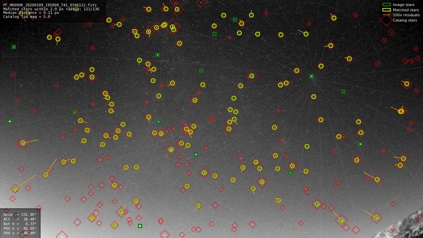
Global Meteor Network 11

Figure 10. Calibration details for the GMN station ES0002 with the 3.6 mm lens. Left: Astrometric calibration residuals using the radial distortion model.
Right: Photometric calibration residuals. The vignetting coefficient is given in radians per pixel.

Figure 11. Calibration details for the all-sky Global Fireball Observatory station at Tavistock, Ontario, Canada, co-located with the Canadian Meteor Orbit
Radar and Canadian Automated Meteor Observatory. Left: Astrometric calibration residuals. A radial distortion with odd terms up to the 7th order was used
and the asymmetry correction was applied. Right: Photometric calibration residuals.

significant again, it is common to resolve several discrete fragments The first step is to correlate meteor observations from multiple
which can be picked separately if desired. In most cases only the stations and produce candidate groups of observations of a common
brightest fragment is tracked. meteor. All observations are divided into 24-hour bins, with the bin
 After observations from all stations are reduced, the trajectory edges set at 12:00 UTC. Observations within a 10 second window
and orbit is computed using the Monte Carlo method described in (from the middle of the meteor) and from cameras 5 km to 600 km
Vida et al. (2020a). The solution may be inspected and outlier picks distant to one another which have overlapping fields of view are
improved or removed. We present a full example of a manually examined as a group to produce candidate trajectories.
reduced fireball trajectory in the Results section 3.4.

2.7 Automated trajectory estimation
 The FOV overlap is checked by confirming that vectors passing
All meteor observations are accumulated on the central GMN server through the center of the focal plane of each pair of cameras is visible
and trajectories are computed every 6 hours. For every night and in the other camera’s field of view for heights between 50-130 km.
station, a list of meteor detections (time, right ascension, declina- Given the location of a reference camera (camera A), its Earth-
tion, magnitude for every frame) and a calibration file are produced. centered inertial (ECI) coordinates at the time when the meteor
The calibration files contain the camera location and pointing infor- was observed (see Appendix D1 of Vida et al. 2020a), and ECI unit
mation. All observations which did not pass the recalibration step vector ˆ of the center of the focal plane, the point along that
described in section 2.5 are rejected. unit vector at height ℎ above ground can be computed as

MNRAS 000, 1–30 (2020)

12 D. Vida et al.

Figure 12. An example of an automated astrometry calibration generated
by RMS for an image showing many matched stars in the night of January
9/10, 2020 for the station HR000K (3.6 mm lens). Yellow circles indicate
matched image and catalog stars, with the residuals plotted as yellow lines at
100× their actual value. Green boxes are detected stars and red diamonds are
 Figure 14. Variation of the photometric offset in the night of January 9,
catalog stars that were not matched because either a bright star was missing
 2020 for the station HR000K in Croatia. The thin lines indicate the one
in the GAIA DR2 catalog, or a fainter star was not picked up by the star
 sigma confidence interval of the photometric fits (around ±0.15 ). The
extractor.
 Moon entered the field of view at 00:00 UTC.

 If the previous checks are satisfied, an intersecting planes tra-
 jectory solution is computed for these two stations using the method
 described in Vida et al. (2020a). Solutions which have meteor end
 heights higher than begin heights are rejected, as well as all meteors
 which begin outside the 50-150 km range, and end higher than 130
 or below 20 km. Note that these filters will exclude some deeply pen-
 etrating fireballs, but those are rare and are designed to be manually
 reduced in the GMN workflow.
 Next, the average velocity as seen from both stations separately
 is computed. The solution is rejected if they do not agree within
 25%, or are outside the 3-73 km s−1 range. If all checks are satisfied
 again, the pair of observations is added as a candidate trajectory.
 Next, all pairs with common observations are merged into groups
 of three or more observations if they occurred within a 10 second
 window and have radiants within 15° from one another. Groups of
 station detections where the maximum convergence angle between
 all observations is smaller than 3° are discarded.
Figure 13. Pointing direction variation color coded by time since the begin-
ning of the night of January 9, 2020 for station HR000K in Croatia. The final complete trajectory solution is done using the Monte
 Carlo method of Vida et al. (2020a), using a minimum of 40%
 of points from the beginning of the trajectory to compute the ini-
 tial velocity. This method will automatically estimate timing offsets
 | | cos between observations. Ten Monte Carlo runs are done to estimate
 = + arcsin , (2) the uncertainties, and 20 runs are used if the convergence angle is
 +ℎ
 cos smaller than 15°. Trajectories are rejected if they do not produce
 = ( + ℎ) , (3) heliocentric orbits or the trajectory minimization procedure does
 cos 
 not succeed. Successful solutions are checked for bad individual
 = + ˆ , (4)
 measurements from individual stations (those outside the 2 con-
where is the range from the station to , is the angle between fidence interval). If bad observations are found, they are removed
 , the centre of the Earth, and , is the elevation of the centre of and the solution is recomputed. This process continues until stable
the focal plane above horizon, and is the distance from the center set of observations is reached. In practice, only 1 or 2 points get
of the Earth to the surface of the WGS84 ellipsoid at the latitude of trimmed from the ends of the trail which are usually obvious out-
the camera (see equation D1 in Vida et al. 2020a). Finally, we can liers produced by an overzealous detection algorithm. All stations
check if this point is visible in the second camera’s field of view by where the root mean square deviation (RMSD) of their observations
testing if the angle between ˆ and − is smaller than half of is larger than 2 arc minutes are rejected. If there are three or more
the diagonal angle of the field of view. Note that this method assumes stations, observations that have an RMSD two times larger than the
a larger circular field of view circumscribed around (drawn outside median of all other RMSD’s are excluded from the solution, unless
of) the actual smaller rectangular FOV, but it prevents unphysical the RMSD is less than 0.5 arc minutes. If at any point only one
trajectory solutions. single-station observation satisfying the conditions above remains,

 MNRAS 000, 1–30 (2020)

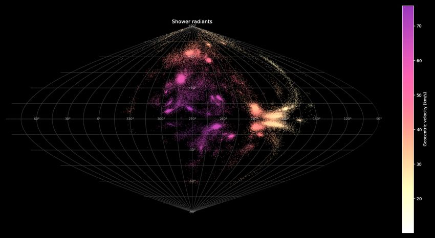
Global Meteor Network 13

Figure 15. A mosaic of video frames of a fireball observed on January 22, 2020 over Southwestern Ontario. Red squares mark raw frame cutouts produced by
the RMS fireball detector, while the background is reconstructed from an FF file. a) The early part of the fireball. Red crosses indicate pick points on the current
(large cross) and previous (smaller red crosses) frames, red round markers indicate locations of stars while the green area indicates pixels that will be used for
photometry. The large yellow circle with annulus represents the cursor pick location. b) Wake becomes visible. c) A flare occurs necessitating a manual pick.
d) Two distinct fragments visible at the end.

the trajectory candidate is rejected. The final average velocity is dated with new observations from stations that were late to upload
again checked to ensure it is within the 3-73 km s−1 range. their data.
 Using the astrometric solution to provide the range to each sta-
tion per frame, the photometric mass is computed by integrating the
100 km range-corrected light curve using the bolometric power of a 3 RESULTS
zero-magnitude meteor 0 = 1210 W (appropriate for Sony HAD
EX-View sensors, which might be different for IMX291; Weryk & Since the beginning of semi-regular operations in December 2018,
Brown 2013) and a dimensionless luminous efficiency = 0.7% the GMN recorded a total of ∼ 220, 000 meteors for which orbits
(Campbell-Brown et al. 2013). The light curve for integration is were computed (up to mid-2021). Every night-time annual meteor
computed by combining observations from all stations and only shower of significance for the satellite impact hazard (Moorhead
taking the brightest estimate. This method helps reduce effects of et al. 2019) was observed by the GMN over that period.
saturation if a meteor was observed by a more distant camera that Figure 16 shows the geocentric velocity distribution of all ob-
did not saturate. GMN cameras saturate at around magnitude −1 served meteors, sporadic meteors, and the top eleven showers with
(depending on the angular velocity of the meteor); thus meteors the most observed meteors. Meteoroids on asteroidal orbits ( > 3)
with brighter peak magnitudes will have underestimated photomet- make up 28.5% of the data set, Jupiter-family type (2 < < 3)
ric masses. orbits 20.5%, and Halley-type ( < 2) orbits 51.0%. We note that
 these raw percentages are subject to a significant observational bias
 Next, a check is made to determine if the meteor began or
 as GMN is a brightness-limited survey; namely the mass limit for
ended within the field of view of at least one camera. This is done by
 fast meteors is much smaller than for slower meteors. At the high
propagating the meteor trajectory forward/backward by two frames
 velocity extreme, GMN detects meteoroids two to three orders of
from the observed end/begin point in the image plane and checking
 magnitude smaller in mass than at the low velocity end. As a result
if the resulting coordinates are within the image. If only a portion
 the raw number of detections is richer in fast showers.
of the meteor was observed, the resulting photometric mass is only
 We note that at speeds below 20 km s−1 there are few known
the lower limit and is so flagged.
 meteor showers and that shower meteors constitute only 5.4% of
 A final set of filters is applied to each event before it is recorded
 those orbits. Generally, shower meteors constitute 51.1% and 41.9%
in the GMN database:
 of Jupiter-family and Halley-type comet orbits, respectively. A total
 of 10,400 Perseids, 10,200 Geminids, 6,200 Orionids, 5,400 Tau-
 • The meteor needs to be observed on at least 6 frames by the rids (North and South combined), and 2,000 Southern -Aquariids
station which observed it the longest. have been observed, among the top showers. However, again, these
 • A minimum convergence angle of 5° is imposed. represent raw observed numbers and since meteor showers typically
 • Orbits with eccentricities larger than 1.5 are rejected. have a shallower size frequency distribution than the sporadic back-
 • Orbits with geocentric radiant errors > 2° or geocentric veloc- ground (Koten et al. 2019), they will tend to be over represented
ity errors > 10% are rejected. relative to sporadics at a given speed.
 • Meteors that start above 160 km or end below 20 km are re- Figure 17 shows the dependence of the meteor peak magnitude
jected. with apparent initial velocity. A clear positive correlation of brighter
 magnitudes with higher velocities can be seen; at 20 km s−1 the
 Finally, meteor shower membership is determined using the average observed peak magnitude is +1.5 , while at 70 km s−1 it is
meteor shower table of Jenniskens et al. (2018) with a fixed angu- −0.5 . This trend is also seen for CAMS meteors (Jenniskens et al.
lar radius of association of 3° and a maximum geocentric velocity 2011), though the magnitude difference in that survey between fast
threshold of 10% (see Moorhead et al. 2020, for more details about and slow meteors is about half the GMN offset. We also note that
this procedure). All computed trajectories and orbits are accumu- compared to the stellar limiting magnitude, peak meteor magnitudes
lated into a table and immediately published on the GMN website. are as much as 4 brighter. This magnitude offset is explained by
Within a window of seven days, the trajectories are continuously up- taking the detection thresholds, a 4-frame duration minimum, noise

MNRAS 000, 1–30 (2020)