The impact of wavelet estimation in 4D inversion - an offshore Brazil case study - CGG
←
→
Page content transcription
If your browser does not render page correctly, please read the page content below
SPECIAL TOPIC: MARINE SEISMIC & EM

The impact of wavelet estimation in 4D inversion —
an offshore Brazil case study
Ekaterina Kneller1*, Ulisses Correia1, Jean-Philippe Coulon1, Laryssa Oliveira1, Paulo de Oliveira
Maciel Junior 2 and Wilson Lisboa Ramos Filho2 demonstrate how wavelet estimation in 4D
inversion in a post-salt turbidite reservoir in the Campos Basin can lead to significant uplift in
the mapping of 4D anomalies.

Introduction                                                             advanced processing technologies available in the industry at the
The development and production of post-salt turbidite reservoirs         time to enhance reservoir monitoring and characterization. The
frequently present a challenge. One effective tool for understanding     baseline survey was acquired in 2005 and the monitor survey
fluids and pressure effects in reservoirs is 4D global inversion. This   in 2018. Both surveys deployed streamer vessels towing 6 km
tool can be used to obtain changes in elastic properties over time,      long cables, 50 m apart, with 480 channels in each cable. A
helping to reduce uncertainty in mapping 4D anomalies. The 4D            configuration of two sources spaced 25 m apart was used. The
global inversion workflow is a multistage process that includes          main objective was to evaluate the 4D seismic signal in post-salt
seismic data preconditioning, wavelet estimation, low-frequency          reservoirs. Processing efforts focused on preserving data ampli-
model building, 3D inversion, and finally a 4D global inversion.         tude and removing source- and receiver-related ghosts. A set of
This inversion algorithm benefits from an iterative and non-linear       pre-stack depth migration (PSDM) imaging techniques, as well
optimization process that greatly improves the 4D interpretation. In     as state-of-the-art time-lag full waveform inversion (TL-FWI)
this work, focusing on a post-salt turbidite reservoir in the Campos     and least-squares (LS) migration technologies, were also applied.
Basin, offshore Brazil, we show how this process can help to better          Furthermore, to improve the repeatability between surveys,
understand the 4D seismic data, bringing a significant uplift in the     seismic conditioning processes were performed prior to the 4D
quality of the mapping of the 4D anomalies. Special attention was        seismic inversion study. These included random noise filtering,
paid to the wavelet estimation process, which played a significant       and structurally consistent filtering, 4D warping and residual
role in this case study. The 4D inversion results helped in the          time-misalignment correction with very small time shifts which
decision-making process for selecting new well locations in the          do not impact the frequency content.
study area. The objective of this work is to demonstrate the benefits
of assessing the impact of the inversion parameters, particularly        Global 4D inversion
wavelets, on 4D interpretation.                                          The main purpose of 4D inversion is to derive a model of
                                                                         the changes in the elastic properties of the reservoir from the
Geological setting                                                       seismic amplitude variations between vintages. The impedances
The field is located in the Campos Basin, in the southeastern            characterize the interval properties of the rocks, while the
region of the Brazilian continental margin. A 6 km wide channel          reflectivity characterizes the contrasts between intervals. The
represents its external geometry, elongated in the NW-SE direc-          result of 4D inversion is the P-Impedance (Ip) volume for the
tion. The production zone comprises Eocene turbidite sandstone           base and monitor surveys and the analysis is performed through
reservoirs deposited in a deep marine environment. The reservoirs        interpretation of the Ip Ratio calculated using the following
have good porosity (29% on average), good absolute permeability          equation:
(2500 mD on average), and a large active aquifer, which is efficient
at maintaining reservoir pressure. The oil gravity is 19° API.           Ip Ratio= 100*(Ip_moni – Ip_base)/Ip_base.
    Although the external geometry of the reservoir is well
resolved using the available 3D seismic data, internal details of        The 4D inversion workflow is a multistep process including:
the oil zone are very difficult to observe owing to the impact of        1. Well-to-seismic calibration and wavelet estimation,
the fluid (oil) in the seismic signal.                                   2. Stratigraphic model building,
                                                                         3. Initial low-frequency model,
4D survey design and seismic processing                                  4. 3D inversion,
This study relates to a time-lapse (4D) seismic processing project       5. 4D inversion as an iterative process with parameter optimi-
performed in 2018/2019, which benefited from all the latest                  zation.

    1
        CGG |   2
                    Petrobras
    *
        Corresponding author, E-mail: ekaterina.kneller@CGG.com
    DOI: 10.3997/1365-2397.fb2021082

                                                                                 FIRST   BREAK   I   VOLUME   39   I   NOVEMBER   2021     45
SPECIAL TOPIC: MARINE SEISMIC & EM
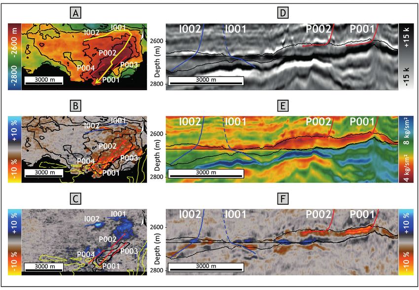
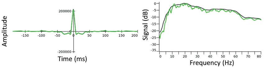
1. Well-to-seismic calibration and wavelet estimation are key In Figure 3 we observe two main differences between statistical
steps in the inversion process because they link seismic amplitude wavelet WV2 and multi-well wavelet WV4. Firstly, WV2 has
and reflectivity derived from elastic properties. Table 1 summa- higher amplitude high-frequency content (20-80 Hz) and, second-
rizes the workflow used for wavelet estimation. All the wavelets ly, WV2 has lower amplitude low-frequency (0-10 Hz) content.
were extracted from the near partial stack (8 degrees). The initial This difference in low frequency content can be interpreted as a
guess is usually based on a zero-phase statistical wavelet (Edgar bias introduced by the use of a short vertical time window for the
and van der Baan, 2011). Wavelet WV1 was estimated for a time wavelet extraction, owing to the limited interval where either the
window of 1 second in the vicinity of three well locations, which logs are available and/or the match between seismic and synthetic
were sufficiently representative of the entire volume (Figure 1). is sufficiently good. To attenuate the secondary lobes that may
The jittering of the frequency spectrum can be stabilized by add- still be observed on the wavelets in the time domain and that can
ing more traces or smoothing the frequency spectra (Figure 1). be interpreted as noise, we decided to use stronger constraints.
The smoothing effect with the use of a 3 Hz moving window For example, WV5 was extracted in the same way as WV4 but
is demonstrated by wavelet WV2 (WV1 with the smoothing using a 10 Hz smoothing window to obtain a smoother phase
applied). Based on a visual evaluation, the smoothing effect is and amplitude spectra. Figure 2C shows the individual wavelets
stronger where the spectrum is ‘steeper’ – the curves diverge and Figure 3 shows the multi-well wavelet for comparison.
between 0 and 7 Hz (Figure 1). Increasing the smoothing attenuates secondary lobes and noise.
Once the statistical wavelet has been obtained, the well-to- Unfortunately, it also has a significant impact on the width of the
seismic tie can be performed and refined. We recommend apply- central lobe, which may affect the vertical resolution, and the low
ing minimal stretch and squeeze editing to the time-depth curve, frequencies (0-5 Hz), which may introduce a bias compared to the
respecting the check-shots or integrated sonic logs. A deterministic WV4 (red) and the WV5 (blue) spectra (Figure 3). We generated
wavelet can then be estimated at each well location with the three wavelet versions for subsequent inversion tests: WV2 – the
amplitude and phase spectra that provide the maximum cross-cor- statistical wavelet with the 3 Hz smoothing window applied, WV4
relation between the seismic and synthetic traces. Figure 2A shows – the constrained well wavelet, and WV5 – the more constrained
the result of wavelet estimation in three wells, W001, W004, and well wavelet, which contains fewer sidelobes and noise. Despite
W006. When the deterministic wavelets are being extracted, the observing the constant component in wavelets WV4 and WV5,
use of constraints (taper, smoothing, averaging between wells) these wavelets were used in the inversion tests to demonstrate the
becomes important, since every mismatch between seismic and possible impact on the inversion result.
well reflectivity impacts the wavelets (Figure 2A). Usually, at
this stage, some wells are excluded from the wavelet estimation 2. Stratigraphic model construction is an important stage in the
process – as is the case for well W006, which was excluded from workflow because the inversion used is layer-based – the average
the analysis owing to a ‘noisy’ individual wavelet, which is an thickness of microlayers and the geometry of the layering must be
indication of the uncertainty in its well-to-seismic calibration. As optimized depending on the seismic resolution and stratigraphic
mentioned above, the extraction process requires some constraints context.
– we applied smoothing of phase spectra in a 3 Hz window
(Figure 2B). The phase was computed in the 4 to 48 Hz frequency 3. Initial low-frequency model building is an essential part
interval and extrapolated out of this interval. Only traces with cor- of 3D inversion to obtain a reliable absolute elastic model
relation coefficients greater than 0.6 were used in the extraction. from the inversion process using five partial angle stacks
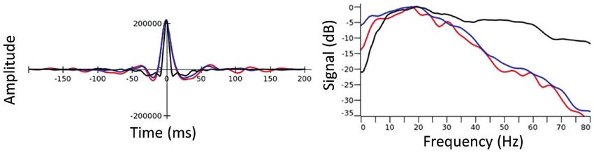
Figure 1 WV1 and WV2. Statistical wavelets and
amplitude spectra without (green, WV1) and with
(black, WV2) smoothing using a 3 Hz moving window.
Short description Parameters Name Complementary
Low-Pass Filter
First guess Statistical wavelets WV1 3-12 Hz
Statistical ‘good looking’ Smooth 3 Hz applied to the WV1 WV2 3-12 Hz
‘Raw’ well wavelets Well wavelets without constraints WV3
Constrained well Well wavelets with soft constraints WV4 1-8 Hz
wavelets
Overconstrained well Well wavelets with harsh WV5 0-6 Hz
Table 1 Wavelet extraction workflow. All the wavelets
wavelets constraints
were extracted from the near partial stack (8 degrees).
46 FIRST BREAK I VOLUME 39 I NOVEMBER 2021
SPECIAL TOPIC: MARINE SEISMIC & EM

                                                                                           Figure 2 A).WV3. Wavelets are estimated with well
                                                                                           data for wells W001, W004 and W006 without using
                                                                                           any constraint or stabilization. B). WV4. Wavelets
                                                                                           are estimated with well data with 3 Hz smoothing.
                                                                                           C). WV5. Wavelets are estimated with well data with
                                                                                           10 Hz smoothing.

                                                                                           Figure 3 Comparison of wavelets. WV2 statistical
                                                                                           wavelet (black), WV4 constrained multi-well wavelet
                                                                                           (red), and strongly constrained multi-well wavelet
                                                                                           WV5 (blue).

                                                                                           Figure 4 Low-pass filters were designed for the three
                                                                                           wavelets. The blue curve is a spectrum of the wavelet,
                                                                                           the black curve is the calculated complementary filter,
                                                                                           and the magenta curve is the low-pass ramp defined
                                                                                           by two frequency values matching the complementary
                                                                                           black spectra. A) for wavelet WV2 – low pass 3-12 Hz,
                                                                                           B) for WV4 – low pass 1-8 Hz, C) for WV5 – low pass
                                                                                           0-6 Hz.

covering incidence angles of up to 36 degrees. Considering             Using the three different wavelets (WV2, WV4, and WV5)
the band-limited seismic data, the main objective is to fill       and their corresponding low-frequency models, based on the
the gap in the low-frequency range that is not present in the      values shown in Figure 4, 3D inversion runs were performed.
seismic data. Figure 4 shows the low-pass complementary            Figure 5 shows a comparison section through the acoustic imped-
filters designed for the wavelets. The statistical wavelet WV2     ance volumes. The inversion with the WV2 statistical wavelet
requires a 3-12 Hz low-pass filter for the initial model. The      (A) demonstrates the strongest low-frequency content compared
constrained multi-well wavelet WV4 requires a 1-8 Hz low-pass      to the inversion using the WV4 (B) and WV5 (C) well wavelets.
filter for the initial model. The additionally smoothed wavelet    The accuracy of the 3D inversion can be numerically evaluated
WV5 requires a 0-6 Hz low-pass filter for the initial model.       through an analysis of the match to the well log values – this is
Adding the wells and the smoothing ‘boosts’ low frequencies        one of the main decision-making criteria in the inversion param-
in the wavelets and means, as a result, that the initial model     eter optimization process. The three inversion tests demonstrate
requires a narrower frequency corridor. The properties required    similar correlation values (around 0.7) between the upscaled
in the inversion were propagated in the stratigraphic model with   impedance logs and inversion results, so, based on this, none of
collocated co-kriging using the seismic velocity as a second       the tests can be judged to be better than the others. The quality
variable.                                                          of the 3D inversion result based on the correlation values alone
                                                                   cannot be used as a criterion for the wavelet choice.
4. 3D Inversion as described by Coulon et al. (2006) is part of
the 4D inversion workflow because it provides the initial model    5. Further analysis was performed through a global 4D inversion
for the 4D inversion.                                              method described by Lafet et al. (2008) using the workflow

                                                                           FIRST   BREAK   I   VOLUME     39   I   NOVEMBER       2021          47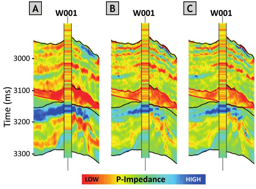
SPECIAL TOPIC: MARINE SEISMIC & EM

                                                                                                       Figure 5 3D inversion results intersecting well W001
                                                                                                       A) with statistical wavelet WV2 and initial 3-12 Hz
                                                                                                       model, B) with constrained multi-well wavelet WV4
                                                                                                       and initial 1-8 Hz model, C) with strongly constrained
                                                                                                       multi-well wavelet WV5 and initial 0-6 Hz model.

shown in Figure 6. As for the 3D inversion process, 4D inver-
sion minimizes a cost function using a Simulated Annealing
procedure. However, it is adapted to the multi-vintage setting
and allows user control over the level of 4D coupling between
inverted elastic attributes. The objective is to find a global solu-
tion that simultaneously optimizes the match between the input
angle stacks for all vintages and the corresponding synthetics.
Time-lapse coupling is achieved by restricting the range of the
perturbations between successive surveys according to user-spec-
ified constraints, based on physical knowledge of the 4D changes.
This makes it possible to reduce the inversion non-uniqueness
and limit the solution space. These user-defined bounds integrate
several pieces of information summarizing the degree of con-
fidence in the initial model, the reliability of the rock-physics
information linking successive surveys, the magnitude of the 4D           Figure 6 Global 4D inversion of multiple seismic vintages and angle stacks with 4D
signal and other geological interpretation constraints.                   corridor constraints for coupling inverted attributes between successive surveys. A
     In this study, we only show the acoustic part of the 4D              wavelet is an input for each partial stack (modified from Lafet et al., 2008).
inversion as it is the main variable for analysing the 4D signature
in the context of the field, with a dominant fluid change response,       uses the well wavelets WV4 and WV5. The main 4D anomalies –
no temperature effect, no compaction, no strong pressure change,          softening (red) and hardening (blue) – are less prominent against
and no salinity issues. The challenge of 4D inversion parametri-          the increasing 4D noise in tests B and C. The strong 4D response
zation lies in the absence of direct numerical quality controls           outside the reservoir interval (defined by the black horizons) – in
(i.e, matching with well logs as in 3D inversion), which would            Figure 7 – prompted us to check the seismic data more carefully
allow informed decision making about the choice of parameter              and we found a difference between the frequency content of the
values. In this study, and considering the information available,         Base and Monitor in the 0-10 Hz interval (Figure 8). This observa-
we decided to start from an identical initial elastic model for the       tion inspired a series of tests with different wavelets for the Base
different vintages (no initial 4D difference was introduced). This        and Monitor in the global 4D inversion. In the initial tests, the same
initial model is based on the results obtained from a preliminary 3D      wavelets that were created for the Base vintage were also used for
inversion of the Base vintage. Out of curiosity to see the impact of      the Monitor vintage even though this could potentially introduce
the estimated wavelets, the 4D inversion test was performed with          more bias in the results due to the absence of any production
the three different wavelets. Test A is a 4D inversion with statistical   effects in the well logs. Tests D, E, and F in Figure 7 correspond
WV2, test B uses the constrained WV4 and test C uses the strongly         to the inversion with different wavelets for the Base and Monitor.
constrained WV5. Figure 7 shows the sections through the Ip Ratio         By using different wavelets it is possible to significantly attenuate
volumes from these 4D inversion tests.                                    the 4D noise outside the reservoir because they help to compensate
     The Ip Ratio extracted from inversion A with statistical wavelet     for the difference in the bandwidth of Base and Monitor. When the
WV2 contains a lower-amplitude signal outside the reservoir               statistical wavelets are used – comparing tests A and D – we can
compared to the Ip Ratio from inversion tests B and C which               see the significant uplift in the amplitude of the signal compared

48      FIRST   BREAK   I   VOLUME   39   I   NOVEMBER   2021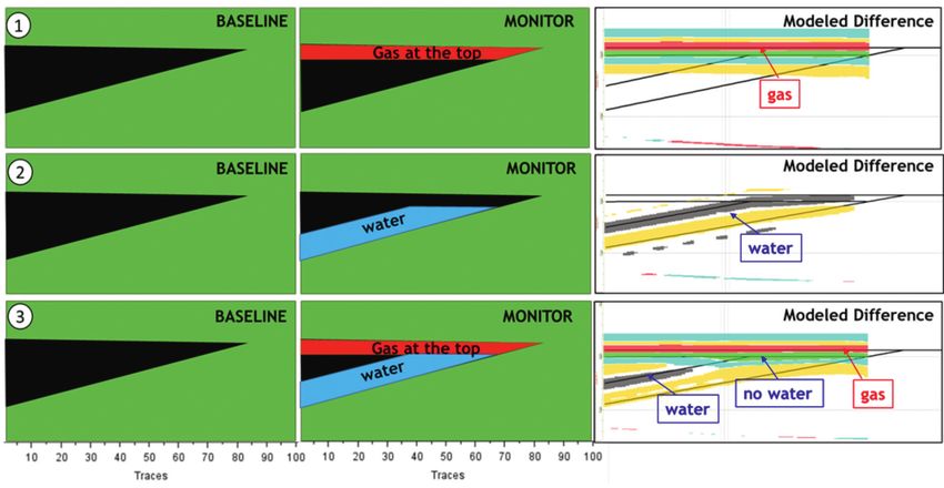
SPECIAL TOPIC: MARINE SEISMIC & EM

to the noise level. The 4D noise tends to decrease also for tests E                       Currently, the drainage strategy for this reservoir consists
and F compared to tests B and C respectively, but at the same time,                   of four horizontal producing wells positioned at the top of the
in other locations, noise is introduced by the wavelet difference.                    channel complex away from the oil-water contact level.
This is explained by the wavelet estimation bias when using well                          A large aquifer maintains the effective pressure in the res-
data in a short estimation window, in addition to the impact of the                   ervoir close to its original value, but two injection wells, which
constraints and smoothing. Both these factors impact mostly the                       are also horizontal, and positioned in the northern portion of the
low-frequency part of the spectra where the difference between                        field, inject water to help to maintain pressure and guide the
Base and Monitor was observed. To evaluate the 4D inversion                           hydrocarbon flow. However, the low efficiency of the injecting
tests quantitatively, the ratio of 4D Energy inside and outside the                   wells during the period between the seismic surveys resulted in
reservoir was used as a metric. First, for every test, we extracted                   the formation of a gas cap just above the production wells in the
the map of the energy for the reservoir interval. Then, both Top                      upper part of the structure.
and Base horizons were shifted 150 ms below to obtain a similar                           The producer wells started operating between 2008 and 2015,
interval outside the reservoir and the energy was estimated there.                    while the injectors have been operating since 2011. The 4D seismic
These values of energy were calculated using Impedance Ratio                          analysis between 2005 and 2018 is therefore suitable for evaluating
volumes and Table 2 shows the average values for each test in the                     the dynamic behaviour of the reservoir. The pressure regime is
representative rectangular area consisting of 230,000 traces. Test D,                 globally stable and only a few isolated compartments may be
4D inversion with the use of statistical wavelets extracted separate-                 relevant.
ly for the Base and Monitor, was selected as the best result based                        For this reservoir, oil sands are typically of lower impedance
on the 4D Energy ratio and was used in the subsequent analysis.                       than the shales, resulting in a negative seismic amplitude
The energy inside the reservoir for this test is 5.48 times stronger                  response at the top of the reservoir and positive response at the
than the energy outside the reservoir, while in other tests this metric               base (Figure 9D). The 3D acoustic impedance section shows
has lower values – it decreases drastically when we analyse tests
B, C, E, and F which use the well wavelets. The tests using the
different wavelets for the Base and Monitor (D, E, F) have higher
values of the metric compared to the tests with the same wavelets
for the Base and Monitor (A, B, C). This analysis shows that the
bias in wavelet estimation can have a strong negative impact on
the 4D inversion result adding 4D noise to results and can be
unidentifiable in the preceding 3D inversion tests.

Interpretation of results
The whole 4D inversion parametrization process required
close interaction between the geophysicists and the interpreters
because, unlike 3D inversion, no detailed quantitative quality
control analysis is available. All impedance variations observed
in the 4D inversion results are directly linked to the effects of
field production, and require validation by a field specialist. In
the light of that, we based all our final geological interpretation
work on the best test we obtained from the sensitivity analysis
we made - test D. We should also mention that the interpretation
itself is a fundamental component of this whole inversion
process.
                                                                                      Figure 7 4D inversion test results. A) Common WV2 wavelet for Base and Monitor B)
                                                                                      Common WV4 wavelet for Base and Monitor C) Common WV5 wavelet for Base and
                                                                                      Monitor D) Different WV2 wavelets for Base and Monitor E) Different wavelets for
 4D inversion         Energy inside        Energy                Ratio of             Base and Monitor, WV4, F) Different wavelets for Base and Monitor, WV5. The black
 test                 reservoir            outside               Energy inres/        horizons define the top and the base of the reservoir formation interval, and the red
                                           reservoir             outres               horizons limit the top of the oil leg, without a gas cap in the vicinity of the well, and
                                                                                      the base of the oil leg merged with the oil-water contact.
 A                    2.24                 0.47                  4.77

 B                    1.81                 0.70                  2.59

 C                    1.96                 0.72                  2.72

 D                    2.41                 0.44                  5.48

 E                    1.74                 0.69                  2.52

 F                    1.81                 1.71                  1.06
Table 2 The ratio of energy inside and outside the reservoir for ratio impedance in   Figure 8 Frequency spectra of the Base and Monitor seismic datasets showing a
4D inversion tests.                                                                   difference in the 0-7 Hz range.

                                                                                                  FIRST    BREAK     I   VOLUME      39   I   NOVEMBER        2021          49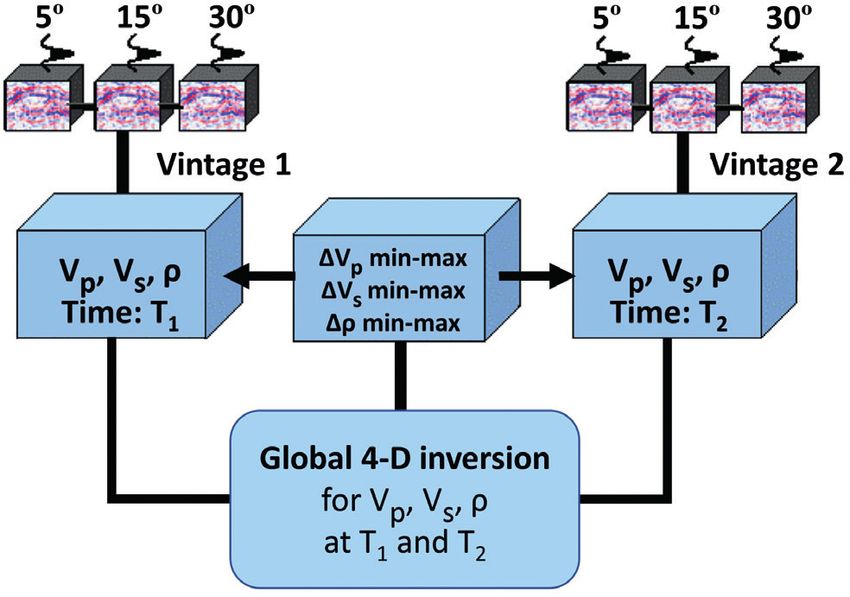
SPECIAL TOPIC: MARINE SEISMIC & EM

Figure 9 4D geophysical interpretation and integration with reservoir management. A) Reservoir top depth map. B) Maximum negative values of the relative acoustic impedance
ratio, indicating impedance decreases, in a 10 m layer at the top of the reservoir. C) Maximum positive values of the relative acoustic impedance ratio, indicating impedance
increases, in a 25 m layer at the base of the reservoir. D) 3D seismic amplitude of the Base. E) 3D acoustic impedance from 3D seismic inversion of the Base. F) 4D inversion
acoustic impedance ratio. In map A, the yellow line represents the arbitrary line location through selected wells for the sections on the right. In maps B and C, the yellow polygons
represent the outline of regions with low 4D seismic repeatability (high NRMS above the reservoir) due to surface obstructions. In sections D, E, and F the black lines are the top
and base reservoir, and the oil-water contact. In both map and section views, the injectors are in blue (I001, I002) and the producers are in red (P001, P002, P003, P004).

                                                                                                                            Figure 10 Illustrative 4D seismic amplitude modelling
                                                                                                                            for different wedge model scenarios: gas saturation
                                                                                                                            increases at the top (1), water saturation increases at
                                                                                                                            the base (2), and both simultaneously (3).

the strong seismic response to the fluid content, indicating the                                 The softening anomalies at the top of the reservoir (Figures 9B
oil-water contact (Figure 9E).                                                               and 9F) are related to an increase in gas saturation. Because of
    As a result of the high-quality data, it was possible to identify                        the depletion history of the field and the temporary increase in
anomalies mainly related to changes in fluid saturation in the 4D                            the produced gas-oil ratio, the most likely interpretation is that
seismic response. In terms of other reservoir property changes                               pressure has declined below the bubble point, causing gas to
which could result in a 4D seismic response, the effects of tempera-                         break out of the solution. Therefore, this gas that is out of solution
ture and salinity can be ignored and the pressure drop is also small,                        migrates upwards to the top of the reservoir and forms a secondary
but significantly, initial pressure was just above the bubble point.                         gas cap. In Figure 9F we can see differences in the intensities of

50        FIRST    BREAK      I   VOLUME     39   I   NOVEMBER       2021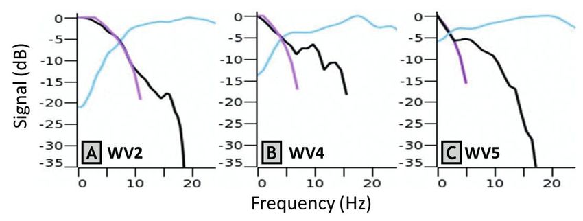
SPECIAL TOPIC: MARINE SEISMIC & EM

this softening effect, which may be related to lower depletion and       to detect the softening and hardening anomalies associated with
gas saturation observed in well P002 when compared to producer           increases in gas and water saturation, respectively. In addition to
P001. Through interpretation of this volume, we can evaluate             the difference in reservoir thickness, the observed difference in
different reliability scenarios for the continuity of the anomaly        these anomalies may also be related to less gas saturation at the top
corresponding to the gas layer, at the time of the Monitor survey.       of the structure at well P002, as previously stated.
Using 4D seismic data to gain insight into the gas distribution and          The results for this reservoir show significant movement of
understand its cause played a significant role in field management.      the oil-water contact on the northern and eastern sides of the field.
     In addition to the 4D anomalies related to the presence of          On the other hand, there is no apparent water movement in the
gas, there are also anomalies associated with the presence of            central part between wells I002 and P002, suggesting there may
water in the lower portions of the oil zone. In Figures 9C and 9F,       be additional drilling opportunities there.
blue areas indicate increases in impedance, which is the result of
water replacing oil. Furthermore, the limit of the anomaly on the        Conclusions
eastern flank is conformable with structure and movement in the          In this study, we presented a detailed description of 4D global
oil-water contact. These changes can be observed around injec-           inversion, paying particular attention to wavelet extraction, which
tion wells I001 and I002 (Figure 9C, north), where the water             helped us to understand its impact on the 4D interpretation. In this
was injected into a thin oil zone and shifted the oil-water contact      way, it was possible to minimize inversion artifacts and improve
towards the producing wells on top of the structure (Figure 9A,          confidence in the results. We have shown the merits of a stepwise
dark red area). The advancement of water, especially from the            approach in parametrizing the 4D inversion, particularly for
aquifer, is observed where the water saturation increases near           handling the wavelets. We also demonstrate that the consistent and
the producing wells yielding an impedance increase (hardening            highly reliable 4D results we obtained, coupled with a thorough
anomaly) in the blue areas (Figure 9C and 9F).                           geological interpretation, enabled us to achieve a better understand-
     In Figure 9F, on the right of injector well I002 (also in Fig-      ing of the dynamic behaviour of the turbidite sandstone reservoir.
ure 9B), there is a small region with a local impedance decrease
(negative values, softening anomaly) interpreted as an overpressure      Acknowledgments
caused by injection in a locally compartmentalized region. Although      The authors would like to thank Petrobras and CGG for permission
there is a discontinuity in the top of the reservoir along the section   to publish this article. They would also like to thank Vitor Mello,
between injecting wells I001 and I002, the compartmentalization          from Petrobras, for his help with Figure 10 of this article that
could not be identified using only the 3D data (Figures 9D and 9E).      greatly supported the discussion in the interpretation of results.
     The increases in acoustic impedance observed in Figure 9F
close to the oil-water contact denote the rising of this surface         References
towards the producing region. However, it is interesting to note that    Coulon, J.P., Lafet Y., Deschizeaux, B., Doyen, P.M. and Duboz, P.
below well P001 there is no hardening effect like the one observed           [2006]. Stratigraphic elastic inversion for seismic lithology discrim-
below well P002, even though production from these wells                     ination in a turbiditic reservoir, SEG Annual Meeting, Expanded
showed a similar increase in water saturation between the Base               Abstracts, 2092-2096, New Orleans, US.
and Monitor surveys. According to a fluid substitution modelling         Edgar, J.A. and van der Baan, M. [2011]. How reliable is statistical wave-
based on a representative reservoir well (Figure 10), the 4D data            let estimation? Geophysics, 76(4), July-August 2011; P. V59-V68, 11
was not expected to be of sufficient resolution to simultaneously            figs. 10.1190/1.3587220.
detect changes related to the softening at the top of the reservoir      Lafet, Y., Roure, B., Doyen, P.M., Bornard, R. and Buran, H. [2008].
and a hardening just below well P001. On the other hand, below               Global 4-D seismic inversion and fluid prediction. 70th EAGE
producing well P002, where the reservoir is thicker, it is possible          Conference & Exhibition, Rome, Italy, 9-12 June 2008.

                                                                                  FIRST   BREAK    I   VOLUME   39   I   NOVEMBER   2021        51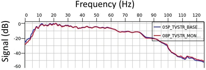
You can also read