The Noninvasive Analysis of Paint Mixtures on Canvas Using an EPR MOUSE - MDPI
←
→
Page content transcription
If your browser does not render page correctly, please read the page content below
heritage

Article
The Noninvasive Analysis of Paint Mixtures on
Canvas Using an EPR MOUSE
Elizabeth A. Bogart † , Haley Wiskoski † , Matina Chanthavongsay † , Akul Gupta † and
Joseph P. Hornak *
 Magnetic Resonance Laboratory, Center for Imaging Science, Rochester Institute of Technology, Rochester,
 NY 14623, USA; eab3609@rit.edu (E.A.B.); hew3641@rit.edu (H.W.); matina.chanth@gmail.com (M.C.);
 akulguptax@gmail.com (A.G.)
 * Correspondence: jphsch@rit.edu; Tel.: +1-585-475-2904
 † These authors contributed equally to this work.

 Received: 6 February 2020; Accepted: 8 March 2020; Published: 12 March 2020

 Abstract: Many artists create the variety of colors in their paintings by mixing a small number
 of primary pigments. Therefore, analytical techniques for studying paintings must be capable of
 determining the components of mixtures. Electron paramagnetic resonance (EPR) spectroscopy is
 one of many techniques that can achieve this, however it is invasive. With the recent introduction of
 the EPR mobile universal surface explorer (MOUSE), EPR is no longer invasive. The EPR MOUSE
 and a least squares regression algorithm were used to noninvasively identify pairwise mixtures of
 seven different paramagnetic pigments in paint on canvas. This capability will help art conservators,
 historians, and restorers to study paintings with EPR spectroscopy.

 Keywords: paint mixture analysis; electron paramagnetic resonance spectroscopy (EPR), low
 frequency electron paramagnetic resonance spectroscopy (LFEPR); EPR mobile universal surface
 explorer; EPR MOUSE; noninvasive EPR of paintings; unilateral EPR of paintings

1. Introduction
     Electron paramagnetic resonance (EPR) spectroscopy is one of a vast number of spectroscopic
analytical techniques [1–10] used by art conservators, historians, and restorers to study paintings.
EPR spectroscopy probes magnetic energy levels associated with unpaired electrons in matter, and
is therefore useful for investigating paramagnetic, ferro/ferrimagnetic, and free radical containing
pigments. The utility of EPR spectroscopy to the art community has been established. EPR spectroscopy
has been used to study rock paintings [11], wall paintings [12], and individual pigments [13–17].
EPR spectroscopy is particularly well suited for studying ancient pigments, as many of these were
either transition metal or free radical based. Conventional high frequency EPR (HFEPR) spectrometers
operate at 9 GHz and have a limit of detection of 1012 spins/mT of spectral linewidth [18], or 0.3 ppb
for a 1 mT linewidth sample. Unfortunately, HFEPR is invasive, limiting the utility of EPR in the
study of precious paintings. It is only recently that a low frequency EPR (LFEPR) spectroscopy was
developed that made EPR spectroscopy noninvasive for 30 cm wide paintings [19,20]. The more recent
development of an EPR mobile universal surface explorer (MOUSE) [21], has made EPR spectroscopy
truly noninvasive for all sample size paintings and made the instrument portable for true in situ
investigations. The EPR MOUSE performs a contact analysis of a bulk sample, obtaining a signal from
a 3 mm diameter, 1.5 mm thick disc on the surface.
     No single analytical technique alone can determine all possible paint analytes under all possible
conditions. Successful studies often rely on complementary techniques [22–26]. Mixtures of paints
make the determination of pigments more challenging for any technique. Artists often work with

Heritage 2020, 3, 140–151; doi:10.3390/heritage3010009                          www.mdpi.com/journal/heritage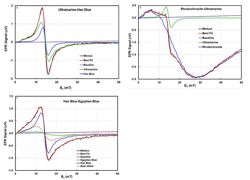
Heritage 2020,33 FOR PEER REVIEW
Heritage2020, 1412
small palette of primary paint colors and mix them to produce the many unique colors in their
apaintings.
small palette of primary
For example, paintMonet
Claude colors had
andamix them
palette ofto
sixproduce
primarythe many
colors thatunique colors
he mixed in their
to produce
paintings. For example, Claude Monet had a palette of six primary colors that he
the many colors in his masterpieces [27]. Deconvolution of complex spectral line components frommixed to produce
the many colors
mixtures in his performed
is routinely masterpieces [27].
with Deconvolution
HFEPR spectroscopyof complex
[28–30], spectral
but it has line components
never from
been reported
mixtures is routinely performed with HFEPR spectroscopy [28–30], but it has never
using the surface coil and unilateral magnet combination found in the EPR MOUSE. Demonstrating been reported
using the surface
the ability of the coil
EPRand unilateral
MOUSE magnetmixtures
to analyze combination found ininthe
of pigments EPRonMOUSE.
paint Demonstrating
canvas will provide art
the ability of the
conservators, EPR MOUSE
historians, andtorestorers
analyze mixtures of pigments
with another in paint on
noninvasive, canvas will provide
complementary art
analytical
conservators, historians, and restorers with another noninvasive, complementary analytical
technique for studying paintings [31,32]. This study specifically answers the question; can the EPR technique
for studying
MOUSE paintings
be used [31,32]. the
to determine Thiscomponents
study specifically answers
of a paint mixturethespectrum?
question; can the EPR MOUSE be
used to determine the components of a paint mixture spectrum?
2. Background
2. Background
Electron paramagnetic resonance spectroscopy is based on the absorption of photons of energy E
Electron paramagnetic resonance spectroscopy is based on the absorption of photons of energy
and Larmor frequency ν by matter with unpaired electrons when placed in an external magnetic field
E and Larmor frequency ν by matter with unpaired electrons when placed in an external magnetic
(B). The relationship between ν and B is given by Equation (1) and depicted in Figure 1, where β and h
field (B). The relationship between ν and B is given by Equation (1) and depicted in Figure 1, where
are physical constants known as the Bohr magneton and Planck’s constant, respectively, and the Landé
β and h are physical constants known as the Bohr magneton and Planck’s constant, respectively, and
g factor is an intrinsic constant of matter containing unpaired electrons.
the Landé g factor is an intrinsic constant of matter containing unpaired electrons.
EE==hhνν==ggββ BB (1)
(1)
Therelationship
The relationshipbetween
betweenννand andBBisismore
morecomplex
complex when
when thethe atoms
atoms have
have unpaired
unpaired nuclear
nuclear spinspin
or
or multiple unpaired electrons, but Equation (1) will suffice for an understanding of our
multiple unpaired electrons, but Equation (1) will suffice for an understanding of our presentation. presentation.
Continuouswave
Continuous waveEPR
EPRspectra
spectraare
arerecorded
recordedby bysending
sendingaafixed
fixedννinto
intothe
thesample
samplewhile
whilescanning
scanning
B.AAspectral
B. spectralabsorption
absorptionappears
appearswhen
whenEquation
Equation(1)(1)isissatisfied.
satisfied. Spectral
Spectral absorptions
absorptions appear
appear as as first
first
derivatives of an absorption as a function of B because magnetic field modulation and phase
derivatives of an absorption as a function of B because magnetic field modulation and phase sensitive sensitive
detection at
detection at the
the modulation
modulation frequency
frequency areare employed
employed to to improve
improvethe thesignal-to-noise
signal-to-noise ratio
ratio (SNR)
(SNR) in in aa
spectrum[33].
spectrum [33].
Figure 1. EPR Energy level diagram depicting the relationship between the absorbed energy, first
derivative signal, and magnetic field.
Figure 1. EPR Energy level diagram depicting the relationship between the absorbed energy, first
derivative
The size ofsignal, and magnetic
the EPR signal is field.
related to the population difference between the two spin levels
and given by Boltzmann statistics [33]. The greater the population difference, the larger the signal.
The size of the EPR signal is related to the population difference between the two spin levels
and given by Boltzmann statistics [33]. The greater the population difference, the larger the signal.Heritage 2020, 3 142
Defining N− and N+ as the respective number of electron spins in the upper and lower energy levels, k
as Boltzmann’s constant, and T as the absolute temperature of the sample,
N− hν
= e−( kT ) (2)
N+
HFEPR spectrometers operate at ν = 9 GHz and scan B between approximately 100 and 600 mT.
LFEPR spectrometers generally operate at ν < 500 MHz and scan 0 < B < 50 mT. Equation (2) tells us
that HFEPR has a larger signal and thus smaller limit of detection than LFEPR.
Continuous wave EPR spectra are recorded by sending a fixed ν into the sample while scanning
B. A spectral absorption appears when Equation (1) is satisfied. Spectral absorptions appear as first
derivatives of an absorption as a function of B because magnetic field modulation and phase sensitive
detection at the modulation frequency are employed to improve the SNR in a spectrum [33].
It can be inferred from Equation (2) that the EPR signal is proportional to the number of spins [33].
Lifetime effects and spatial inhomogeneity in B give width to an EPR signal. All other acquisition
factors being constant, the number of spins is proportional to the area under an absorption peak. For
equal spin concentration samples, the one with the narrowest linewidth will have the lower LOD. EPR
spectra of mixtures of equal molar concentrations of two different spin types with different linewidths
will retain the relative LOD due to linewidth differences. In pigments, this may be further complicated
by the signal being due to an impurity as in Victoria green [34], or a non-stoichiometric free radical as
in charcoal [35].
Paramagnetic materials are distinguished from each other by their g factor, peak-to-peak linewidth
(ΓPP ), and any splitting pattern from interactions between electron and nuclear spins. The g factor and
ΓPP are more challenging to quantify with LFEPR because the ΓPP is often approximately equal to the
sweep width of B and a clear estimation of the signal baseline is not always available to determine the
g factor. Additionally, samples with nuclear spin and/or multiple unpaired electrons create spectra that
are more challenging to interpret.
The invasive nature of HFEPR spectroscopy and the poorer limit of detection of LFEPR spectroscopy
may have hindered the development of EPR for studying paintings. Advances in electronics and the
introduction of the EPR MOUSE, which can examine any 3 mm diameter spherical cap shaped area of
an infinite size painting, changes the viability of EPR for studying paintings. Demonstrating the ability
of the EPR MOUSE to identify mixtures of two pigments will further advance the viability of EPR
spectroscopy for studying paintings.
3. Materials and Methods
Seven pigments were chosen to make the paints used in this study: charcoal (C) (Kingsford),
Egyptian blue (EB) (CaOCuO(SiO2 )4 , Kremer Pigments), Han blue (HB) (BaOCuO(SiO2 )4 , Kremer
Pigments), rhodochrosite (RC) (MnCO3 , Kremer Pigments), terracotta red (TCR) (clay flowerpot),
ultramarine (UM) (Na8 Al6 Si6 O24 S3 , Old Holland), and blue vitriol (BV) (CuSO4 ·5H2 O, J.T. Baker).
Ultramarine and charcoal are respectively sulfur and carbon centered free radicals. Han blue and
Egyptian blue are isomorphs, differing only in the presence of barium or calcium ions, and contain
paramagnetic Cu(II) ions. Blue vitriol is also a paramagnetic Cu(II) ion pigment. Even though these
three pigments contain Cu(II) ions, their EPR properties are very different. Rhodochrosite and terracotta
red contain paramagnetic Mn(II) and Fe(III), respectively. These pigments were selected because they
have a known LFEPR signal. [20] The set contains pigments with a variety of g factors, ΓPP values, and
signal amplitudes, as it is these properties and not colors that matter in EPR spectroscopy analysis.
These properties represent the range of possible values and determine the ease of distinguishing
between any two pigments in a mixture spectrum.
The pigments were used for seven standard paints. The Ultramarine blue was a premixed,
commercial linseed oil-based paint. The Han Blue, Egyptian Blue, and Rhodochrosite powders were
used as is, while the blue vitriol, charcoal, and terracotta red were crushed and sieved to have particlesHeritage 2020, 3 143
Heritage 2020, 3                                                                                          144

where kc is a constant for a given coil. For the MOUSE surface coil kc = 2.65 mm−1 , and S reaches 95%
of its maximum value by 1.15 mm. This signal profile drove our use of more impasto-like swatches.
The spectral acquisition parameters for all standards and mixtures are summarized in Table 1. All spectra
for a swatch were reproducible. All aspects of the spectrometer were controlled by LabVIEW® (National
Instruments) code. Spectra were imported into Microsoft Excel for display and analysis.

                            Table 1. EPR MOUSE spectral acquisition parameters.

                                        Parameter                     Value
                                     Spectral Points                   1000
                                      Dwell Time                    215 ms/pt
                                     Time Constant                     0.3 s
                                      Sweep Start                    0.05 mT
                                       Sweep End                    50.48 mT
                                        Step Size                  0.05048 µT
                                 Operating Frequency (ν)           421.8 MHz
                                  Modulation Frequency               10 kHz
                                 Modulation Amplitude                0.22 mT
                                  Number of Averages                   4-10

     The analysis of the mixtures consisted of first creating standard spectra (Si (x)) where i represents
the standard number and x the data point in the spectrum for each of the standard swatches. These
spectra were a result of averaging at least four individual, x = 1000 point spectra together to achieve a
desirable SNR. Spectra of the mixture swatches (Mj,k (x)) for each of the 21 pairwise mixtures (j,k) of the
seven pigments. Additional single mixture spectra were recorded where j=k to check the performance
of the algorithm.
     The algorithm calculated a trial mixture spectrum (T(x)) defined by Equation (4), where Ai is the
amount of the ith spectrum contributing to the trial spectrum.
                                              X
                                      T (x) =     (Ai Si (x)) + So (x)                                   (4)
                                                   i

So (x) is a term added to the summation of Equation (4) to account for the possibility of a small linear
baseline drift during the acquisition of the mixture spectrum. This term has the form So (x) = mx+b
where m is the slope and b the intercept.
      The sum of the square of the residuals between each point of Mj,k (x) and T(x) is given by Equation (5).
                                              X                    2
                                         R=       M j,k (x) − T (x)                                       (5)
                                               x

The algorithm determines the combination of Ai , m, and b necessary to minimize R, giving a least
squares method. The algorithm was implemented in Microsoft® Office Excel and the Ai values
determined for each mixture spectrum using the Solver option with the Generalized Reduced Gradient
(GRG) nonlinear solving method selected. The Solver was constrained to keep Ai ≥ 0, seeded with
Ai = m = b = 0, and terminated with a constraint precision of 0.00001. Excel was chosen because its
availability and widespread use on personal computers. The fraction of each standard paint swatch
spectrum in a mixture swatch spectrum was reported as
                                                         A
                                                   fi = P i                                               (6)
                                                         i Ai

     To convert fi to a mole fraction, it is necessary to know the molar concentration of each standard
paint swatch and either have equal swatch thicknesses or in the case of unequal thicknesses, knowledge
of the spatial signal per unit quantity of sample of sensitivity of the MOUSE surface coil. This was not
attempted because of the need to know the exact spatial sensitivity of the MOUSE and the challenge of
making swatches with equal thickness.
Heritage 2020, 3 145
4. Results
The seven standard spectra recorded with the EPR MOUSE are presented in Figure 3, and the ΓPP
and zero crossing of the spectra are presented in Table 2. The standards contain spectra with similar and
different ΓPP and zero crossing, thus providing a good test of the algorithm. The ΓPP values are slightly
different than those reported by Javier and Hornak [20]. The differences are attributed to the (1) ν = 421
MHz for the MOUSE and ν = 271 MHz for the 2 cm surface coil, and (2) less homogeneous B of the
Heritage 2020, 3 FOR PEER REVIEW 8
unilateral magnet on the MOUSE compared to the solenoidal magnet used with the 2 cm surface coil.
Figure 3. LFEPR spectra of the seven standard paint samples recorded at 421.8 MHz using the
Figure
EPR 3. LFEPR spectra of the seven standard paint samples recorded at 421.8 MHz using the EPR
MOUSE.
MOUSE.
Table 4. fi values for the calculated spectral components of two component swatches.*.Heritage 2020, 3 146
Table 2. Spectral properties of the seven standard spectra.
Pigment Zero Crossing (mT) ΓPP (mT)
Ultramarine Blue 14.79 2.56
Han Blue 14.53 3.66
Egyptian Blue 13.96 10.85
Terracotta Red 13.05 6.19
Rhodochrosite 10.48 23.63
Charcoal 15.07 0.92
Blue Vitriol 13.75 7.31
These seven spectra were used as the standard spectra in the analysis algorithm. The results from
the analysis are separated into two groups. The first is when the mixture spectrum Mj,k is composed of
a single pigment (j=k). Table 3 summarizes the fi values for each of the seven possible components
in the seven Mj,k spectra. This group served as a test of the algorithm that was designed to identify
multiple components to identify single component spectra.
Table 3. f i values for the calculated spectral components of single component swatches *.
Component
Swatch Spectra C TCR HB EB RC UM BV
Charcoal 0.99 0.00 0.00 0.00 0.00 0.00 0.00
Terracotta Red 0.00 0.99 0.00 0.00 0.00 0.00 0.01
Han Blue 0.00 0.00 1.00 0.00 0.00 0.00 0.00
Egyptian Blue 0.00 0.00 0.00 0.99 0.01 0.00 0.01
Rhodochrosite 0.00 0.00 0.00 0.04 0.96 0.00 0.00
Ultramarine 0.01 0.00 0.00 0.00 0.00 0.99 0.00
Blue Vitriol 0.02 0.00 0.02 0.04 0.00 0.00 0.92
* fi values rounded to the nearest 0.01.
For this single component (j = k) group, the algorithm identified the correct component by
returning a fraction greater than 0.92 in all cases. In five of the cases, the fraction was greater than or
equal to 0.99. In the remaining two cases, rhodochrosite and blue vitriol, the fractions were respectively
0.96 and 0.92. Since all of these swatches were made from single component paints, the deviation from
1.0 must be attributed to the presence of low frequency spectral noise mimicking the spectra of minor
components. To the eye, all spectra fit adequately with f = 1.0 for the actual component, but minor
differences caused by noise cause a better fit with a few percent of other spectra.
The results from the second group of mixture spectrum Mj,k occur when j , k. Table 4 summarizes
the fi values for each of the seven possible components in the 21 Mj,k spectra.
For the 21 swatches in the two-component j , k group, the algorithm correctly identified the two
primary components in all cases. In six of the 21 mixtures, only the two components were found. In five
mixtures, a single extra component was found. In seven mixture spectra, there were two extra minor
components; in two mixture spectra, there were three extra minor components; in a single mixture
spectrum, there were four extra minor components. The presence of these extra minor components
in the fit was again attributed to spectral noise. As with all spectral deconvolution techniques, SNR
affects the ability to discriminate between analytes with similar spectral characteristics. The larger
the noise and closer its frequency to that of the signal frequency, the more difficult the discrimination
between analytes. The two mixtures with the smallest component ΓPP difference, UM-HB and TCR-BV,
had no minor components identified. There was no correlation with zero crossing similarity and
extra components. Both of these observations are characteristic of a random noise process. It should
be possible to decrease the noise by using additional signal averaging as well as increasing the time
constant and dwell time acquisition parameters, thus increasing the scan time of a spectrum.Heritage 2020, 3 147
Table 4. fi values for the calculated spectral components of two component swatches *.
Component
Swatch Spectra C TCR HB EB RC UM BV
Rhodochrosite-Charcoal (1) 0.68 0.00 0.00 0.00 0.32 0.00 0.00
Han Blue-Charcoal (2) 0.66 0.00 0.19 0.05 0.00 0.07 0.03
Egyptian Blue-Charcoal (3) 0.32 0.00 0.00 0.68 0.00 0.00 0.00
Terracotta Red-Charcoal (4) 0.43 0.55 0.00 0.00 0.00 0.01 0.01
Rhodochrosite-Terracotta Red (5) 0.00 0.61 0.00 0.00 0.38 0.00 0.01
Han Blue-Terracotta Red (6) 0.00 0.67 0.33 0.00 0.00 0.00 0.00
Egyptian Blue-Blue Vitriol (7) 0.00 0.00 0.00 0.70 0.02 0.00 0.28
Ultramarine-Blue Vitriol (8) 0.00 0.00 0.00 0.27 0.05 0.03 0.65
Ultramarine-Han Blue (9) 0.00 0.00 0.60 0.00 0.00 0.40 0.00
Blue Vitriol-Charcoal (10) 0.43 0.00 0.00 0.00 0.00 0.00 0.57
Ultramarine-Charcoal (11) 0.53 0.00 0.00 0.00 0.01 0.46 0.00
Rhodochrosite-Han Blue (12) 0.00 0.02 0.37 0.06 0.51 0.05 0.00
Egyptian Blue-Rhodochrosite (13) 0.00 0.01 0.00 0.40 0.58 0.00 0.01
Blue Vitriol-Rhodochrosite (14) 0.00 0.02 0.00 0.00 0.44 0.00 0.55
Rhodochrosite-Ultramarine (15) 0.00 0.03 0.01 0.00 0.83 0.14 0.00
Han Blue-Egyptian Blue (16) 0.00 0.00 0.49 0.27 0.05 0.00 0.19
Han Blue-Blue Vitriol (17) 0.00 0.00 0.29 0.00 0.03 0.04 0.64
Egyptian Blue-Terracotta Red (18) 0.03 0.63 0.00 0.31 0.00 0.00 0.03
Egyptian Blue-Ultramarine (19) 0.00 0.01 0.02 0.56 0.02 0.28 0.10
Terracotta Red-Blue Vitriol (20) 0.00 0.59 0.00 0.00 0.00 0.00 0.41
Terracotta Red-Ultramarine (21) 0.00 0.78 0.00 0.00 0.00 0.16 0.06
* fi values rounded to the nearest 0.01.
Quantitative EPR is challenging [37], and quantitative EPR with a surface coil and unilateral
magnet, such as found in the EPR MOUSE, is most challenging process. For this reason, the focus is not
on attaining fi ≈ 0.5 for two component mixtures. Instead, the metric of success is correctly identifying
the two components of a mixture having the two largest fi values.
Three examples of the fit to the mixture spectra are presented in Figure 4. These examples were
chosen from three general classes of results: (1) only two major fi value, (2) two major and other minor fi
values, and (3) two major and one significant minor fi value. The first example is the mixture spectrum
for ultramarine and Han blue and the best-fit spectrum consisting of the depicted standard spectra
of ultramarine and Han blue. The algorithm found that only the two components were necessary to
attain the best fit. Perhaps the need for only two standard spectra is attributed to the slightly larger
signal and narrow ΓPP values of the components.
The second example is the mixture spectrum for rhodochrosite and ultramarine and the best-fit
spectrum consisting of the depicted standard spectra of ultramarine and Han blue. The algorithm found
that four components were necessary to attain the best fit: two major components 0.83 rhodochrosite
and 0.14 ultramarine, and two minor components 0.03 terracotta red and 0.01 Han blue. The need for
the minor components is attributed to the noise level in the spectrum.
The final example is the mixture of Han Blue and Egyptian Blue. The regression algorithm found
0.49 Han blue, 0.27 Egyptian blue, 0.05 rhodochrosite, and 0.19 blue vitriol. The primary components
found were the correct ones, but the 0.19 blue vitriol value was unexpectedly large. Perhaps there is
some abnormal background baseline drift noise that is best fit with the combination of the wider ΓPP
blue vitriol and rhodochrosite contributions. In either event, it is difficult to tell the difference between
the best fit with these four components and just Han Blue and Egyptian Blue by using the naked eye.
The least squares fit shows that the fit with all four is slightly better.Heritage2020,
Heritage 2020,33 FOR PEER REVIEW 10
148
Figure 4. LFEPR analysis spectra of the mixtures (a) ultramarine-Han blue, (b) rhodochrosite-
Figure 4. LFEPR
ultramarine, and (c) analysis spectra of blue.
Han blue–Egyptian the mixtures a) ultramarine-Han
Each plot compares the mixture,blue, b) and
best fit, rhodochrosite-
individual
ultramarine,
component and c) Han blue–Egyptian blue. Each plot compares the mixture, best fit, and individual
spectra.
component spectra. .
The under-layer results are presented in Table 5. They show that the MOUSE and algorithm were
able toThe under-layer
identify the tworesults are presentedultramarine
major components: in Table 5. and
Theycharcoal.
show that the MOUSE
Knowing and
that the algorithm
swatch was
were able to identify the two major components: ultramarine and charcoal. Knowing that
clearly blue, one would conclude that there had to be a charcoal under layer. As with many of the the swatch
was clearly
other blue,
swatches, one would
it appears conclude
as noise that
in the there had
spectrum to bean
caused a erroneous fi = 0.03
charcoal under layer. As for
value with many of
terracotta
the which
red, other was
swatches, it appears
not present in the as noise in the spectrum caused an erroneous fi = 0.03 value for
sample.
terracotta red, which was not present in the sample.
Table 5. fi values for the calculated components of ultramarine over charcoal swatch *.
Component
Table 5. fi values for the calculated components of ultramarine over charcoal swatch.*.
Swatch Spectra C TCR HB EB RC UM BV
Component
Ultramarine Over Charcoal 0.37 0.03 0.00 0.00 0.00 0.60 0.00
Swatch Spectra C TCR HB EB RC UM BV
* fi values rounded to the nearest 0.01.
Ultramarine Over Charcoal 0.37 0.03 0.00 0.00 0.00 0.60 0.00
* fi values rounded to the nearest 0.01.
The technique will work equally well on these pigments in paintings, provided there is a reasonable
Theno
SNR and technique
reactionswill workorequally
between well onofthese
decomposition pigmentsin in
the pigments thepaintings, provided
mixture [38]. Thickerthere
impastois a
reasonable
technique SNR and
paintings no reactions
should be easierbetween or decomposition
than thinner of theaspigments
paint applications, in the
there is more mixture
pigment in [38].
the
Thicker
active impasto
volume technique
of the MOUSEpaintings should
surface coil. The be easier than
technique thinner
works well paint applications, asequal-volume
with approximately there is more
pigmentofinpigments.
mixtures the active volume
Future of can
studies thedetermine
MOUSE the surface coil.
limit of The technique
detection works
and spatial well with
sensitivity with
approximately
more equal-volume
disproportionate mixtures.mixtures of pigments. Future studies can determine the limit of
detection and spatial sensitivity with more disproportionate mixtures.
5. Conclusions
Our results demonstrate that by using the EPR MOUSE and the least-squares regression algorithm,
it5.isConclusions
possible to identify from a library of seven spectra the correct single or mixture of two pigments
that areOurpresent
resultsin demonstrate
a 3 mm diameter
that and up to 1.5
by using themm
EPRthick regionand
MOUSE of athe
painting. Additionally,
least-squares the
regression
algorithm, it is possible to identify from a library of seven spectra the correct single or mixture of twoHeritage 2020, 3 149
approach was demonstrated on one under layer, showing that the pigments do not need to be mixed or
have a visible surface presence. The MOUSE is nondestructive and because it can look at any sample
size, the size of a painting is not an issue and the technique is noninvasive. A single spectrum that is
representative of the components in a sample is recorded in as little as four minutes.
The construction cost of the EPR MOUSE and spectrometer was approximately 40,000 USD, or at
the lower end of the price of analytical instruments used to study paintings. The analysis does not
require purchase of expensive mathematical programming and analysis packages, as the algorithm is
implemented in Microsoft® Excel.
Although not explicitly demonstrated, there are two features of the MOUSE worth mentioning.
First, it is portable and therefore can examine paintings in situ. Second, it can be used for spectral
imaging by rastering the MOUSE across a painting [21,39].
Two negatives of the EPR MOUSE are that it is a contact analysis and its current low SNR.
The former cannot be changed, but latter can be improved by signal averaging and improvements
to the hardware. Random lower frequency noise may affect the algorithm’s ability to discriminate
between two pigments with similar g factors and ΓPP values.
There is still a need for further technique development work to answer the following questions:
Is the technique quantitative such that specific mole fractions of pigments can be determined within
a mixture? Will it work equally well on mixtures of three or four pigments? Will it work equally
well on a larger set of standard spectra? These questions can best be answered by partnering with
art conservators, historians, and restorers. Despite these questions, the analysis works for one or two
paramagnetic pigments with an LFEPR signal, so it will complement techniques that are more suitable
for organic based pigments.
Author Contributions: Conceptualization, J.P.H.; Data curation, E.A.B., H.W., M.C., A.G. and J.P.H.; Formal
analysis, E.A.B., H.W., M.C., A.G. and J.P.H.; Funding acquisition, J.P.H.; Investigation, E.A.B., H.W., M.C.,
A.G. and J.P.H.; Methodology, J.P.H.; Project administration, J.P.H.; Resources, E.A.B. and J.P.H.; Software, J.H.;
Supervision, J.P.H.; Validation, E.A.B., H.W., M.C., A.G. and J.P.H.; Visualization, E.A.B., H.W., M.C., A.G. and
J.P.H.; Writing – original draft, J.P.H.; Writing – review & editing, E.A.B., H.W., M.C. and J.P.H. All authors have
read and agreed to the published version of the manuscript.
Funding: This research received no external funding. M. Chanthavongsay acknowledged support from the
National Science Foundation REU program under project 1658806.
Conflicts of Interest: The authors declare no conflict of interest.
References
1. Giorgi, L.; Nevin, A.; Comelli, D.; Frizzi, T.; Alberti, R.; Zendri, E.; Piccolo, M.; Izzo, F. In-situ technical study
of modern paintings-Part 2: Imaging and spectroscopic analysis of zinc white in paintings from 1889 to 1940
by Alessandro Milesi (1856–1945). Spectrochim. Acta. A 2019, 219, 504–508. [CrossRef]
2. Rosi, F.; Cartechini, L.; Sali, D.; Miliani, C. Recent trends in the application of Fourier Transform Infrared
(FT-IR) spectroscopy in Heritage Science: From micro- to non-invasive FT-IR. Phys. Sci. Rev. 2019, 4. [CrossRef]
3. Brosseau, C.L.; Rayner, K.S.; Casadio, F.; Grzywacz, C.M.; Van Duyne, R.P. Surface-enhanced raman
rpectroscopy: A Direct method to identify colorants in various artist media. Anal. Chem. 2009, 81, 7443–7447.
[CrossRef]
4. Janssens, K.; Dik, J.; Cotte, M.; Susini, J. Photon-based techniques for nondestructive subsurface analysis of
painted cultural heritage artifacts. Acc. Chem. Res. 2010, 43, 814–825. [CrossRef]
5. Calligaro, T.; Gonzalez, V.; Pichon, L. PIXE analysis of historical paintings: Is the gain worth the risk?
Nucl. Instrum. Methods B 2015, 363, 135–143. [CrossRef]
6. Cotter, M.J. Neutron Activation Analysis of Paintings: Autoradiography following neutron irradiation
provides information for authentication and restoration and reveals the existence of underpaintings
undetected by other means. Am. Sci. 1981, 69, 17–27.
7. Lehmann, R.; Wengerowsky, D.J.; Schmidt, H.J.; Kumar, M.; Niebur, A.; Costa, B.F.O.; Dencker, F.;
Klingelhöfer, G.; Sindelar, R.; Renz, F. Klimt artwork: Red-pigment material investigation by backscattering
Fe-57 Mössbauer spectroscopy, SEM and p-XRF. STAR 2017, 3, 450–455. [CrossRef]Heritage 2020, 3 150
8. De Meyer, S.; Vanmeert, F.; Vertongen, R.; Van Loon, A.; Gonzalez, V.; Delaney, J.; Dooley, K.; Dik, J.;
Van der Snickt, G.; Vandivere, A.; et al. Macroscopic x-ray powder diffraction imaging reveals Vermeer’s
discriminating use of lead white pigments in Girl with a Pearl Earring. Sci. Adv. 2019, 5, 1971–1979.
[CrossRef]
9. Prati, S.; Fuentes, D.; Sciutto, G.; Mazzeo, R. The use of laser photolysis-GC-MS for the analysis of paint cross
sections. JAAP 2014, 105, 327–334.
10. Presciutti, F.; Perlo, J.; Casanova, F.; Glöggler, S.; Miliani, C.; Blümich, B.; Brunetti, B.G.; Sgamellotti, A.
Noninvasive nuclear magnetic resonance profiling of painting layers. Appl. Phys. Lett. 2008, 93, 033505.
[CrossRef]
11. Rowe, M.W. Dating of rock paintings in the Americas: A word of caution. In Pleistocene Art of the World;
Clottes, J., Ed.; Société Préhistorique Ariège-Pyrénées: Tarascon-sur-Ariège, France, 2012; Volume 60–61,
pp. 573–584.
12. Moretto, L.M.; Orsega, E.F.; Mazzocchin, G.A. Spectroscopic methods for the analysis of celadonite and
glauconite in Roman green wall paintings. J. Cult. Herit. 2011, 12, 384–391. [CrossRef]
13. Christiansen, M.B.; Sørensen, M.A.; Sanyova, J.; Bendix, J.; Simonsen, K.P. Characterisation of the rare
cadmium chromate pigment in a 19th century tube colour by Raman, FTIR, X-ray and EPR. Spectrochim. Acta
Part A Mol. Biomol. Spectrosc. 2017, 175, 208–214. [CrossRef]
14. Gobeltz, N.; Demortier, A.; Lelieur, J.P.; Duhayon, C. Correlation between EPR, Raman and colorimetric
characteristics of the blue ultramarine pigments. J. Chem. Soc. Faraday Trans. 1998, 94, 677–681. [CrossRef]
15. Orsega, E.F.; Agnoli, F.; Mazzocchin, G.A. An EPR study on ancient and newly synthesised Egyptian blue.
Talanta 2006, 68, 831–835. [CrossRef]
16. Raulin, K.; Gobeltz, N.; Vezin, H.; Touati, N.; Lede, B.; Moissette, A. Identification of the EPR signal of S2 − in
green ultramarine pigments. Phys. Chem. Chem. Phys. 2011, 13, 9253–9259. [CrossRef]
17. Lakshmi Reddy, S.; Udayabashakar Reddy, G.; Ravindra Reddy, T.; Thomas, A.R.; Rama Subba Reddy, R.;
Frost, R.L.; Endo, T. XRD, TEM, EPR, IR and Nonlinear Optical Studies of Yellow Ochre. J. Laser Opt. Photonics
2015, 2, 120. [CrossRef]
18. Wertz, J.E.; Bolton, J.R. Electron Spin Resonance; Chapman and Hall: London, UK, 1986; p. 497.
19. Switala, L.E.; Ryan, W.J.; Hoffman, M.; Javier Santana, S.; Black, B.E.; Hornak, J.P. A Wide-Line Low Frequency
Electron Paramagnetic Resonance Spectrometer. Concepts Magn. Reson. 2017, 47B, e21355. [CrossRef]
20. Javier, S.; Hornak, J.P. A Non-Destructive Method of Identifying Pigments on Canvas Using Electron
Paramagnetic Resonance Spectroscopy. JAIC 2018, 57, 73–82.
21. Switala, L.E.; Black, B.E.; Mercovich, C.A.; Seshadri, A.; Hornak, J.P. An Electron Paramagnetic Resonance
Mobile Universal Surface Explorer. J. Magn. Reson. 2017, 285, 18–25. [CrossRef]
22. Zoleo, A.; Nodari, L.; Rampazzo, M.; Piccinelli, F.; Russo, U.; Federici, C.; Brustolon, M. Characterization of
pigment and binder in badly conserved illuminations of a 15th-century manuscript. Archaeometry 2014, 56,
496–512. [CrossRef]
23. Monico, L.; Janssens, K.; Cotte, M.; Sorace, L.; Vanmeert, F.; Brunetti, B.G.; Miliani, C. Chromium speciation
methods and infrared spectroscopy for studying the chemical reactivity of lead chromate-based pigments in
oil medium. Microchem. J. 2016, 124, 272–282. [CrossRef]
24. Marinescu, M.; Emandi, A.; Duliu, O.G.; Stanculescu, I.; Bercu, V.; Emandi, I. FT-IR, EPR and SEM–EDAX
investigation of some accelerated aged painting binders. Vib. Spectrosc. 2014, 73, 37–44. [CrossRef]
25. Vandivere, A.; Wadum, J.; van den Berg, K.J.; van Loon1, A.; The Girl in the Spotlight research team. From
‘Vermeer Illuminated’ to ‘The Girl in the Spotlight’: Approaches and methodologies for the scientific (re-)
examination of Vermeer’s Girl with a Pearl Earring. Herit. Sci. 2019, 7, 1–14. [CrossRef]
26. Anselmi, C.; Vagnini, M.; Cartechini, L.; Grazia, C.; Vivani, R.; Romani, A.; Rosi, F.; Sgamellotti, A.; Miliani, C.
Molecular and structural characterization of some violet phosphate pigments for their non-invasive
identification in modern paintings. Spectrochim. Acta A. 2017, 173, 439–444. [CrossRef] [PubMed]
27. Kendall, R. Monet by Himself ; Kendall, R., Ed.; Cartwell Books, Inc.: Edison, NJ, USA, 2000; p. 327.
28. Flores-Llamas, H.; Ye-Madeira, H. The deconvolution and evaluation of the area under ESR lines. J. Phys. D
Appl. Phys. 1992, 25, 970–973. [CrossRef]
29. Magon, C.J.; Lima, J.F.; Donoso, J.P.; Lavayen, V.; Benavente, E.; Navas, D.; Gonzalez, G. Deconvolution of
the EPR spectra of vanadium oxide nanotubes. J. Magn. Reson. 2012, 222, 26–33. [CrossRef] [PubMed]Heritage 2020, 3 151
30. Słowik, G.P.; Wi˛eckowski, A.B. Determination of the fraction of paramagnetic centers not-fulfilling. The Curie
law in coal macerals by the two-temperature EPR. measurement method. Nukleonika 2015, 60, 389–393.
[CrossRef]
31. Chabbra, S.; Smith, D.M.; Bode, B.E. Isolation of EPR spectra and estimation of spin-states in two component
mixtures of paramagnetics. Dalton Trans. 2018, 47, 10473. [CrossRef]
32. Ren, J.Y.; Chang, C.Q.; Fung, P.C.; Shen, J.G.; Chan, F.H. Free radical EPR spectroscopy analysis using blind
source separation. J. Magn. Reson. 2004, 166, 82–91. [CrossRef]
33. Poole, C.P., Jr. Electron. Spin Resonance, 2nd ed.; John Wiley & Sons: New York, NY, USA, 1983; p. 780.
34. Navas, A.S.; Reddya, B.J.; Nieto, F. Spectroscopic study of chromium, iron, OH, fluid and mineral inclusions
in uvarovite and fuchsite. Spectrochim. Acta Part A 2004, 60, 2261–2268. [CrossRef]
35. Viana, G.A.; Lacerda, R.G.; Freire, F.L.; Marques, F.C. ESR Investigation of Graphite-Like Amorphous Carbon
Films Revealing Itinerant States as the Ones Responsible for the Signal. J. Non Cryst. Solids 2008, 354,
2135–2137. [CrossRef]
36. Asbeck, W.K.; Van Loo, M. Critical Pigment Volume Relationships. Ind. Eng. Chem. 1947, 41, 1470–1475.
[CrossRef]
37. Eaton, G.R.; Eaton, S.S.; Barr, D.P.; Weber, R.T. Quantitative EPR.; Springer: Berlin/Heidelberg, Germany, 2010;
p. 185.
38. Alter, M.; Binet, L.; Touati, N.; Lubin-Germain, N.; Hô, A.-S.L.; François Mirambet, F.; Didier Gourier, D.
Photochemical Origin of the Darkening of Copper Acetate and Resinate Pigments in Historical Paintings.
Inorg. Chem. 2019, 58, 13115–13128. [CrossRef] [PubMed]
39. Switala, L.E.; Ryan, W.J.; Hoffman, M.; Brown, W.; Hornak, J.P. Low Frequency EPR and EMR Point
Spectroscopy and Imaging of a Surface. Magn. Reson. Imaging 2016, 34, 469–472. [CrossRef] [PubMed]
© 2020 by the authors. Licensee MDPI, Basel, Switzerland. This article is an open access
article distributed under the terms and conditions of the Creative Commons Attribution
(CC BY) license (http://creativecommons.org/licenses/by/4.0/).You can also read