Radio Antennas, Feed Horns, and Front-End Receivers - Bill Petrachenko, NRCan EGU and IVS Training School on VLBI for Geodesy and Astrometry
←
→
Page content transcription
If your browser does not render page correctly, please read the page content below
Radio Antennas, Feed Horns, and
      Front-End Receivers
          Bill Petrachenko, NRCan
       EGU and IVS Training School on
       VLBI for Geodesy and Astrometry
                March 2-5, 2013
         Aalto University, Espoo, Finland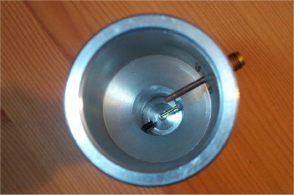
Radiation Basics – Power Flux Density
                Spectral Power Flux Density, Sf (Wm-2H-1),
   is the power per unit bandwidth at frequency, f, that passes through
  unit area. [Subscipt f indicates spectral density, i.e. that the parameter
    is a function of frequency and expessed per unit bandwidth (Hz-1)]

           Sf can be used to express power in bandwidth, δf ,
                     passing through area, δA , i.e.:
                                P = S f ⋅ δA ⋅ δf
   Sf is the most commonly used parameter to characterize the strength
of a source; it is often referred to simply as the Flux Density of the source.

        Because the typical flux of a radio source is very small, a
      unit of flux, the Jansky, has been defined for radio astronomy:
                            1 Jy = 10-26Wm-2Hz-1

 The power from a 1 Jy source collected in 1 GHz bandwidth by a 12 m
  antenna would take about 300 years to lift a 1 gm feather by 1 mm.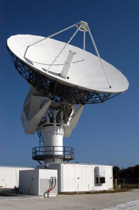
Radiation Basics – Surface Brightness

Surface Brightness, I f (θ , φ ) (Wm-2Hz-1sr-1), is the Spectral Power
  Flux Density, Sf, per unit solid angle (on the sky) radiating from
        direction, (θ , φ ) . (aka Intensity or Specific Intensity)

     Because I f varies continuously with position on the sky,
   it is the parameter used by astronomers for mapping sources.

                  I f is related to Sf according to

                          Sf =   ∫I
                                 ΔΩ
                                      f   dΩ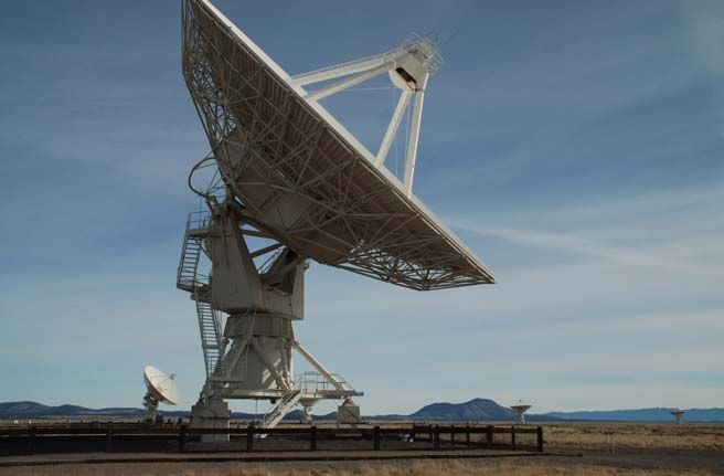
Radiation Basics – Brightness Temperature
                                         Source
                                                        Power generated per
Flux decreases as 1/R2                                  unit solid angle increases
since power per unit area                               proportional to R2 since the
                                      R                 area of the source (in the
is diluted as the distance
from the source increases.                              solid angle) increases as
                                                        the distance from the
                                    Observer            source increases.
   These two opposing effects cancel so that I f is independent of the distance
             from the source and hence a property of the source itself.

   For a Black Body in thermal equilibrium and in the Rayleigh-Jeans limit
(i.e. hν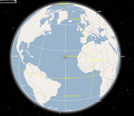
Radiation Basics – Radiative Transfer
                                                        Thermal
        For a Black Body, i.e. a perfect absorber,

                                    ⎛f ⎞
                         I f = 2kTB ⎜ ⎟
                                           2         Incident
                                                                       T
                                    ⎝c⎠
                     (see previous page)

                 For an imperfect absorber
                             2                       Scattered                  Transmitted
                        ⎛f ⎞
             I f < 2kTB ⎜ ⎟
                        ⎝c⎠
                                                                       T
             I f ∝ absorption coefficient

                                                          Absorption is a Lose-lose
               Oxygen                                     effect:
                                                            - the desired signal
For the atmosphere                                        is attenuated
   Imperfect absorption is                                  - thermal noise is added
   why zenith atmosphere                                  to system noise
    at x-band is 3°K and                                         Water vapour
          not 300°K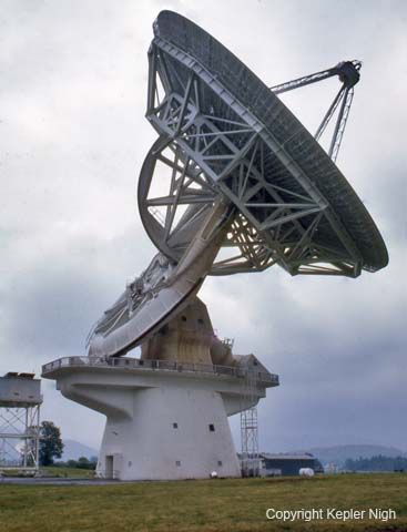
Radiation Basics - Polarization
     The Polarization vector is in the instantaneous direction of the E-field vector

     Linear Polarization             Circular Polarization             Random Polarization
                                                                        Probability of E-field
                                                                        direction

                                                                       Most geodetic VLBI sources
The most efficient detection of linear and circular polarization     have nearly circular distributions,
             signals is with a matched detector.                        i.e. are nearly unpolarized.

Regardless of the input signal, all of the radiated power can be detected with two orthogonal
   detectors, either Horizontal and Vertical linear polarization or Left and Right circular
  polarization. With random polarization this is the only option for detecting all the power.

         Linear Detector                                           Circular Detector

                 e.g. dipole                                           e.g. quadrature combination
                                                  90°      +/-               of dipole outputs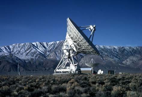
Antenna Basics
•   A Radio antenna is a device for converting electromagnetic radiation in free
    space to electric current in conductors
•   An Antenna Pattern is the variation of power gain (or receiving efficiency)
    with direction.

        Antenna pattern: Dipole antenna      Antenna pattern: Parabolic antenna

•   Reciprocity is the principle that an antenna pattern is the same whether the
    antenna is transmitting or receiving.
     – Transmitting antennas are generally characterized by gain
     – Receiving antennas are generally characterized by effective area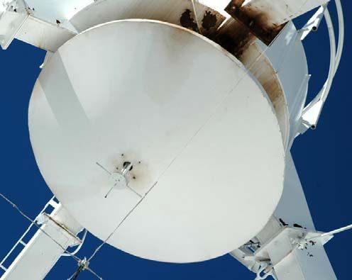
Antenna Gain - Characterizes a Transmitting
                                           Antenna
                                                P (θ , φ )
Antenna gain is defined as, G (θ , φ ) =                   , where
                                                  Piso
        P(θ , φ ) ~ power per unit solid angle transmitted in direction, (θ , φ )
                                                                                              Pin
            Piso ~ power per unit solid angle transmitted by an isotropic antenna, Piso =
                                                                                              4π

For a lossless antenna,      Pout = Pin , hence Glossless = 1 and             ∫ GdΩ = 4π
                                                                            Sphere

An isotropic antenna is a hypothetical lossless antenna radiating uniformly
in all directions, i.e. Giso (θ , φ ) = 1 .
[Note: An isotropic antenna is a useful analytic construct but cannot be built in practice.]

                                                                                   G(θ ,φ )
  The beam solid angle of an antenna is defined as                   ΩA =     ∫
                                                                            Sphere
                                                                                    Gmax
                                                                                           dΩ hence

                                                   4π
                                          ΩA =
                                                  Gmax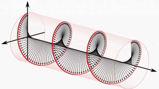
Effective Area – Characterizes a Receiving
                                                     Antenna
    The total power received into area, Ae (θ , φ ) , and bandwidth, BW , is
                           ⎛ Sf   ⎞
              P(θ , φ ) = ⎜⎜      ⎟⎟ Ae (θ , φ )BW             Note: S includes all radiated flux. For an
                           ⎝ 2     ⎠                           unpolarized source, only one half the flux
                              2 P(θ , φ )                      is received per polarized detector. Hence
           ∴ Ae (θ , φ ) =                                     the use of
                                                                             ⎛S⎞
                                                                             ⎜ ⎟   in the equations.
                              S f ⋅ BW                                       ⎝2⎠

              At a particular frequency, Ae (θ , φ ) can be rewritten
                                                             2 Pf (θ , φ )
                                             Ae (θ , φ ) =
                                                                 Sf
                where Pf     (WHz-1)       is the power received per unit frequency

The noise power (per Hz) generated by a resistor at temp, T, can be written Pf = kT .

                                                                         Pf = kT

    Note: It is common to use T as a proxy for Pf , especially in low power/noise situations.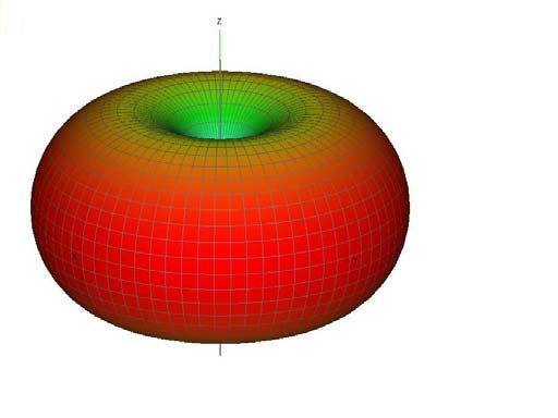
Average effective area
             Antenna Side                                                                Resistor Side
                                                      Black Body cavities
                                   If                    T1                   T2
     Pf =     ∫      Ae (θ , φ )             dΩ
                                    2
            Sphere                                                            R              Pf = kT
                            2
         2kT         ⎛f ⎞
    Pf =
          2
                     ⎜ ⎟
                     ⎝c⎠
                                  ∫ A dΩ e
                                Sphere                Rayleigh-Jeans

At thermodynamic equilibrium, T1=T2 and no current flows between antenna and resistor
                     Antenna Side must equal Resistor Side

                                                             2
                                                2kT    ⎛f⎞
                                              ∴
                                                 2
                                                       ⎜ ⎟
                                                       ⎝c⎠
                                                                   ∫ A dΩ = kT
                                                                 Sphere
                                                                          e

                                                   2
                                     ⎛c⎞                                                λ2
                       ∫         Ω = ⎜ ⎟ = λ                                       Ae =
                                            2
                            Ae d     ⎜f⎟
                     Sphere          ⎝ ⎠                                                4π
                                                  For an isotropic antenna
                                                                     λ2
                                                  Ae (θ , φ ) = Ae =
                                                                     4π
Effective Area Gain
From reciprocity
Ae (θ , φ ) ∝ G (θ , φ )
From earlier results
λ2
Ae = and G =1
4π
Combining these
λ2
Ae (θ , φ ) = G (θ , φ ) = G (θ , φ ) ⋅ Aiso
4π
This allows us to calculate the receiving pattern from the transmitting pattern
and vice versa.Main beam
High Gain Antenna (Gmax>>1) Sidelobes
e.g. Parabolic Reflector Antenna Stray radiation
It was already shown that, in a Black Body cavity, the received spectral density is
I f (θ , φ )
Pf = ∫ Ae (θ , φ ) dΩ = kT
Sphere
2
For a high gain antenna, Ae (θ , φ ) is concentrated in the main beam; hence
I f (θ , φ )
Pf = ∫ Ae (θ , φ ) dΩ = kT
Ω − Beam
2
which implies that I f (θ , φ ) need only cover the main beam for this result to be true.
If a source is smaller than the main beam,
Ω Source
If
Pf = ∫ Ae dΩ = kT
Ω − Beam
2 Ω BeamMain beam
High Gain Antenna (Gmax>>1) Sidelobes
e.g. Parabolic Reflector Antenna Stray radiation
Spectral Power Flux Density, Sf, Relations
If the source is larger than the beam
Ae S f Ω Beam
If
P Re ceived
= ∫ Ae dΩ =
2 Ω Source
f
Ω − Beam
2
If the source is smaller than the beam
If Ae S f
= ∫ dΩ =
Re ceived
P f Ae
Ω − Source
2 2Parabolic Reflector Antenna
Secondary reflector
(aka Sub-reflector)
Sub-reflector support legs
Feed Horn
Antenna positioner Feed Horn Support Structure
Primary reflector
Pedestal
(aka antenna tower)
The antenna reflectors The feed horn converts
concentrate incoming E-M E-M radiation in free
radiation into the focal space to electrical
point of the antenna. currents in a conductor.
The antenna positioner points the antenna at the desired
location on the sky.Aperture Illumination
The ‘Feed Horn’ is itself an antenna with a power pattern that
‘illuminates’ the reflector system. Although the terminology
derives from signal transmission, the feed works equally well,
in a radio telescope, as a receiving element.
Over-illumination: The feed pattern extends well
beyond the edge of the dish. Too much ground
radiation is picked up from outside the reflector.
Under-illumination: The feed pattern is almost
entirely within the dish. There is minimal ground
pick-up but the dish appears smaller than it is.
Optimal-illumination: This is the best balance
between aperture illumination and ground
pick-up. The power response is usually down
about 10 dB (10%) at the edge of the dish.Aperture Illumination Beam Pattern
The beam pattern of the antenna is the Fourier Transform of the aperture
illumination (assuming that the aperture is measured in units of λ).
λ FFT
Aperture illumination
Beam pattern
Depending on the details of the aperture illumination, the Half Power Beam
Width (HPBW) is approximately
λ
HPBW ≈
D
where D is the diameter of the reflector.
The beam becomes narrower as dish becomes larger or λ becomes shorter.
(λ becoming shorter is the same as the frequency becoming larger).Aperture efficiency
The antenna effective area, Ae , can be compared to the antenna
geometric area with the ratio, ηA , being the antenna efficiency, i.e.
Ae = η A Ageo
π
where, for a circular antenna, Ageo = D2 .
4
The antenna efficiency can be broken down into the product of a number
of sub-efficiencies:
η A = η sf ×ηbl ×η s ×ηt ×η p ×η misc
where
• η sf Surface accuracy efficiency (both surface shape and roughness)
• ηbl Blockage efficiency
• ηs Spill-over efficiency
• ηt Illumination efficiency
• ηp Phase centre efficiency
• η misc Miscellaneous efficiency, e.g. diffraction and other losses.Antenna Optics – i.e. reflector configuration
The purpose of the reflector system is to
concentrate the radiation intercepted by the full
aperture (and from the boresite direction) into a
single point.
Axial or Front Feed – aka Prime Focus
The front feed antenna uses a parabaloid primary
reflector with the phase centre of the feed placed
at the focal point of the primary reflector.
Advantages:
• Simple
• No diffraction loss at the sub-reflector (more
important at lower frequencies)
• Only one reflection required leading to less
loss and less noise radiated (minimal benefit if
the reflector material is a good conductor).
Disadvantages:
• Spill-over looks directly at the warm ground.
• Added structural strength required to support
feed plus front end receiver at the prime focusAntenna Optics – i.e. reflector configuration
Off-axis or Offset Feed
The primary reflector is a section of parabaloid
completely to one side of the axis, with the feed
supported from one side of the reflector.
Advantages:
• No aperture blockage (leading to higher
antenna efficiency)
Disadvantages:
• Spill-over looks preferentially toward the
warm ground (especially for high-side feed
support).
• Lack of symmetry.
• Added structural strength required to support
feed plus front end receiver to one side of the
reflector.
• Complications with all-sky positioner for low-
side feed support
• Complications with feed/receiver access for
high-side feed supportAntenna Optics – i.e. reflector configuration
Cassegrain
This is a two reflector system having a hyperboloid
secondary reflector (sub-reflector) between the
prime focus and the primary reflector. The sub-
reflector focuses the signal to a point between the
two reflectors.
Advantages:
• Spill-over past the sub-reflector is
preferentially toward cold sky.
• Minimal structural strength is required since
the sub-reflector is located nearer the primary.
Disadvantages:
• The sub-reflector obscures the prime focus
so it is difficult to achieve simultaneous
operation with a prime focus feed.Antenna Optics – i.e. reflector configuration
Gregorian
This is a two reflector system having a parabaloid
secondary reflector (sub-reflector) located on the
far side of the prime focus. The sub-reflector
focuses the signal to a point between the prime
focus and the primary reflector.
Advantages:
• Spill-over past the sub-reflector is
preferentially toward cold sky.
• The sub-reflector does not obscure the prime
focus so it is easier to achieve simultaneous
operation with a prime focus feed.
Disadvantages:
• Greater structural strength is required since
the sub-reflector must be supported further
away from the primary.Antenna Optics – i.e. reflector configuration
Shaped Reflector System
A shaped reflector system requires optics that
involve more than one reflector, e.g. the
Cassegrain or Gregorian systems. With a shaped
reflector system, the shape of the secondary
reflector is altered to improve illumination of the
primary. To compensate for the distortion of the
secondary, the shape of the primary must also be
changed away from a pure parabaloid.
Advantages:
• Improved efficiency
Disadvantages:
• The reflectors are no longer simple
parabaloids or hyperbaloids but more complex
mathematical shapes. [With the advent of
readily available computer aided design and
manufacture this is no longer a significant
complication.]Antenna Feed – crossed dipole
An antenna feed is itself an antenna. Whereas the reflector system concentrates
radiation from a wide area into a single point, the feed converts the E-M radiation
at the ‘single point’ into a signal in a conductor.
One of the simplest feeds is a crossed
dipole, i.e. a pair of orthogonal ½-λ
350-MHz crossed dipole
dipoles usually located ¼-λ above a
ground plane, e.g. the VLA crossed
dipoles.
75-MHzAntenna Feed - Broadband
A broadband feed can be designed using a series of log periodic dipoles. Log
periodic means that the length and separation of the dipoles increases in a
geometric ratio chosen so that all frequencies are covered. Here we see a
version of the Eleven Feed developed at Chalmers University for VLBI2010.
This version covers 2-12 GHz with a newer version covering 1-14 GHz.
Folded dipoles of the Eleven FeedCrossed dipole - polarization
Each dipole of a crossed dipole is sensitive
to signals with polarization vectors parallel
V-pol dipole
nal
Si
g to the dipole. Two orthogonal dipoles can
receive all the power from an arbitrary
signal.
H-pol dipole
An arbitrary polarization vector
decomposed into orthogonal
components
Circular polarization is formed by combining linear
signals in quadradure (i.e. by adding and subtracting
90°-shift linear polarizations after one of them has been
shifted by 90°). This works easily for narrow band
signals – but the existence of broadband 90°-shifters
+/- (hybrids) also makes it applicable to broadband
signals (like VLBI2010). For this to work well, the
L/R-pol electronics must represent the mathematics
accurately.VLBI works best with circular polarization
As seen from above, the linear polarization orientation for alt/az
antennas varies with geographic location
1 2 3 4 5
3 * 3 1 * 3
For parallel orientations, For orthogonal orientations,
correlated signal is found correlated signal shifts
in the co-pol products, to the cross-pol products
e.g. v1*v2 and h1*h2 e.g. v1*h2 and h1*v2
To avoid the shifting of correlated amplitude between cross- and co-pol products ,
VLBI traditionally uses circular polarization, where correlated amplitude is
independent of relative polarization orientation.Circular Polarization
To avoid noise degradation in the combining network, LNA’s are required
immediately on the outputs of the dipole antennas. Any amplitude or
phase imbalances in the amplifiers or inaccuracies in the 90° phase shifter
or combiners will degrade the generation of circular polarization.
LNA 90°-shift
LNA +/- L/R-polFeed Horns (as used in S/X-band feeds)
A piece of waveguide can be used directly as a feed.
However, because there is a significant mismatch between
the impedence of the waveguide and that of free space,
much of the input radiation is reflected or scattered.
To improve the match the waveguide is often flared and
corrugated.
Dipole antennas act as
probes to convert the
E-M radiation in the
waveguide to a signal
in a cable. Here we see
dual frequency probes
If a septum is inserted in the waveguide
Low frequency
both linear polarizations can be combined
High frequency
to get both circular polarizations without
the need for external circuitry.Antenna Positioners – Alt-az
The antenna positioner is system that points the beam of the antenna toward the area
of sky of interest. There are three main positioner systems: alt-az, equatorial, and X-Y.
Alt-az
This is the workhorse antenna mount for large radio
telescopes. It has a fixed vertical axis, the azimuth
axis, and a moving horizontal axis, the altitude (or
elevation) axis that is attached to the platform that
rotates about the azimuth axis. The azimuth motion
is typically ±270° relative to either north or south
and the elevation motion is typically 5° to 85°.
Advantages:
• Easy to balance the structure and hence
optimum for supporting a heavy structure.
Disadvantages:
• Difficult to track through the zenith due to the
coordinate singularity (key hole).
• Complications with cable management due to
540° of azimuth motion (cable wrap problem).Antenna Positioners - Equatorial
Equatorial
This type of positioner is no longer used for large
antenna’s although it was in widespread use prior to
the advent of high speed real-time computers for
calculating coordinate transformations. It has a fixed
axis in the direction of the celestial pole, the equatorial
axis, and a moving axis at right angles to the
equatorial axis, the declination axis. The declination
axis is attached to the part of the antenna that rotates
around the equatorial axis. The axis motion is
somewhat dependent on latitude but is < ±180° in
hour angle (equatorial) and < ±90° in declination.
Advantages:
• Can be used without computer control – just get
on source and track at the sidereal rate.
• No cable wrap ambiguity
Disadvantages:
• Difficult to balance the structure and hence sub-
optimal for large structures.
• Key hole problem at the celestial pole.Antenna Positioners – X-Y Mount
X-Y Mount
This type of positioner is mainly used for high
speed satellite tracking where key holes cannot be
tolerated. The fixed axis points to the horizon and
hence the only keyhole is at the horizon, which is
too low for tracking. Full sky coverage can be
achieved with ±90° motion in both axes.
Advantages:
• No place where an object cannot be tracked
(i.e. no key holes).
• No cable wrap ambiguity
Disadvantages:
• Structurally difficult to construct (compared
with alt-az).Typical Traditional VLBI Receiver
(S- or X-band)
Antenna Control room
Down
Feed converter
Channelizer
Cable run
Recorder
Formatter
RF IF
Digitizer
LNA
+ LO
Noise Pulse
diode gen.
Maser
• Down-conversion is done in the front end so that
Intermediate Frequency (IF) signals can be transmitted to
the control room on cables. Baseband converter
• The channelizer is an analog function hence it appears Baseband
IF
ahead of the digitizer in the diagram. Channelization is filter
achieved using a set of baseband converters (each LO Locked to
including an LO, single sideband mixer and maser
programmable filter).More Modern VLBI Receiver
(similar to VLBI2010)
Antenna Control room
Feed
Cable run
Channelizer
Recorder
Formatter
Converter
Up/Down
Fiber
Digitizer
LNA
+
Noise Pulse
diode gen.
Maser
• The full analog Radio Frequency (RF) signal is transmitted to the control
using analog over fibre, involving conversions from electrical to optical
and back to electrical.
• Flexible (any frequency) down-conversion is achieved using an Up-
Down converter
• The digitizer is ahead of the channelizer, which is implemented digitally
in a Digital Back End (DBE) as a Polyphase Filter Bank (PFB).Most Modern VLBI Receiver (DBBC3)
Antenna Control room
Feed Cable run
Converter
Channelizer
Digitizer
Recorder
Formatter
Down
LNA
Fiber
Noise
diode
Maser
• Digitization is done immediately after the LNA so that both down-
conversion and channelization are done digitally
• The signal is transmitted to the control room digitally over fibre.Amplification - Low Noise Design
The signal received from a radio source is very weak, e.g. using
P = A S = 2kT
Pff = Aee S ff = 2kTa a
System Noise Budget
a 1 Jy source observed by a 12 m antenna with 50% efficiency will produce an
antenna temperature, TA=0.02° K about 1000 times smaller than typcial system
noise. [See the table below for a breakdown of system noise components.]
Typical antenna
Source of noise Major dependencies
temperature (°K)
Cosmic microwave background 3
Milky Way Galaxy 0-1 frequency, direction
Ionosphere 0-1 time, frequency, elevation
Troposphere 3-30 elevation, weather
Antenna radome 0-10
Antenna 0-5
Ground spillover 0-30 elevation
Feed 5-30
Cryogenic LNA 5-20
Total 16-130Amplification - Low Noise Design
Hence it is important that good low noise design strategies be used, i.e. that the first
amplifier in the signal chain (the one immediately after the feed) has:
• very low input noise, i.e. that it is a cryogenically cooled Low Noise Amplifier
(LNA).
• high gain to dilute the noise contribution of later stages.
G1 ( S + N + N1 )
S+N G1 G2 G1G2 (S + N + N1 ) + G2 N 2
N1 N2
G1G2 S S The second noise
Hence, SNR = =
G1G2 ( N + N1 ) + G2 N 2 N + N + N 2 contribution has been
1 reduced by the first
G1 gain.
For example, if G1=3000 (35-dB) and N2=200°K, N2/G1=0.07°K.Amplification - Gain Compression
It is important that amplifiers operate in the linear range, i.e. output is simply
a multiple of the input (e.g. if input doubles the output must also double).
The 1 dB compression point is an
important amplifier specification. It is a
measure of how large a signal can be
input to an amplifier before significant
non-linear behaviour begins. It occurs at
the input signal level where output
increases 1 dB less than the input. To
guarantee linear operation, systems are
usually designed to operate at least 10
dB below the 1 dB compression point.
Consequenses of non-linear behaviour
Linear operation Saturation
- VLBI signal
disappears at
saturation.
VLBI noise signal - Amplitude modulation
plus cw RFI shifts frequenciesDynamic Range Example
Dynamics Range is the range of amplitudes in which an amplifier can operate.
The lower end is limited by noise performance of the amplifier and the upper end
is limited by gain compression.
For astronomical signals it is expected In following stages, the input signal
that the input signal will be significantly must be significantly above the noise
0-dBm below the first stage LNA input noise. level to avoid further degradation of the
This leaves the full dynamic range noise budget.
available to absorb unexpected signals
IN1dB Second stage compression
like Radio Frequency Interference (RFI).
IN1dB 20-dB DR
-50-dBm
Max linear power
-50-dBm 1% Noise add
30-dB DR
Second stage noise
Tsys Noise
50°K = -80-dBm Dotted lines show the
Follow-on stage operating levels of the
-100-dBm follow on stage.
Astronomical
Signal -110-dBm Gain=30 dB
LNA
10-dB/division
-150-dBmSystem Equivalent Flux Density (SEFD)
SEFD is the flux density that produces, in any particular system, an antenna
temperature equal to the system temperature. It is a figure of merit for the
sensitivity of the antenna/feed/receiver system (SNR=Sf /SEFD). Using
Ae S f η AπD 2
Pf = = kTa and Ae = ,Ta can be expressed as,
2 4
η AπD 2 S f
Ta =
8k
Under the condition Ta = TS it is true by definition that S f = SEFD so that
8kTs
SEFD = Note: SEFD decrease as
η AπD 2 sensitivity increases.
SEFD is very useful in VLBI for predicting the correlated amplitude and SNR, i.e.
ηc S f
Amp =
SEFD1 × SEFD2 SNR = Amp 2 × BW × T
where ηc is the correlator digital processing efficiency and 2xBWxT is the number of
independent samples. Amp is typically 10-4 so 2xBWxT must be very large to get
a good SNR. [Note: The SEFD spec for VLBI2010 is 2500.]Measurement of SEFD
Operationally, the SEFD is determined by measuring the power on and off a
source with a calibrated flux density.
P(on-src)
P(src)
P(off-src) P(on-src) = P(sys)+P(src)
P(sys) P(off-src) = P(sys)
Zero level
Using P(on-src), P(off-src) and the flux of the calibration source, SEFD can be
determined according to:
S f (cal − src )
SEFD =
⎛ Pon − src ⎞
⎜ − 1⎟
⎜P ⎟
⎝ off − src ⎠
Note: The units of P(on-src) and P(off-src) are irrelevant (provided they are both
the same) since only their ratio is used in the equation.Noise Calibration
• Noise calibration measures changes in the power sensitivity.
• A signal of known strength is injected ahead of, in, or just after the
feed, and the fractional change in system power is measured.
• The system temperature is then calculated from the known cal
signal strength as Tcal
Tsys =
⎛ Pon ⎞
⎜ − 1⎟
⎜P ⎟
⎝ off ⎠
• Even if the true value of the Tcal is unknown, the calculated Tsys
values are useful as measures of the relative changes in sensitivity.
• If Tcal is small (≤5% of Tsys), continuous measurements can be made
by firing the cal signal periodically (VLBA uses an 80 Hz rep rate)
and synchronously detecting the level changes in the backend.
• For reliable Tsys measurements
– Tcal must be stable (may require physical temperature control) and
– the system gain ahead of the injection point must be stable.Phase Calibration
The phase calibration system measures changes in system phase/delay.
• This is particularly important for cable delays that can vary with antenna
pointing direction and hence correlate with station position.
A train of narrow pulses is injected ahead of, in, or just after the feed - typically at
the same location as the noise cal signal.
• Since the PCAL signal follows exactly the same path (from the point of
injection onward) as the astronomical signal, any changes experienced by
the calibration signal are also experienced by the astronomical signal.
Feed LNA
+
Noise Pulse
diode gen.
Reference from maserPhase Calibration (cont’d)
Pulses of width tpulse with a repetition rate of N MHz correspond to a series of
frequency tones spaced N MHz apart from DC up to a frequency of ~1/tpulse
• E.g., pulses of width ~50 ps yield tones up to ~20 GHz
• Typical pulse rate is 1 MHz, but it will be 5 or 10 MHz in VLBI2010 (to
reduce the possibility of pulse clipping).
Δt=1/N(MHz) Δf=N(MHz)
PCAL
PCAL
Δt Δf
t f
Time domain representation Frequency domain representation
The PCAL signal is detected in the digital output of the receiver (usually at the
correlator where it is used). The detection can be either in the time domain or the
frequency domain:
• In the frequency domain, a quadrature function at the frequency of the tone
stops the tone so that it can be accumulated thus implementing the tone
extractor.
• In the time domain, averaging of the repetitive pulse periods implements the
pulse extractor with an FFT transforming the result to the frequency domain.Phase Calibration (cont’d)
• Older pulse generators used tunnel or step recovery diodes.
• Newer pulse generators use high-speed digital logic devices.
Precision of the instrumental phase/delay measurements can be no better
than the stability of the phase cal electronics
• Temperature sensitivity of the new phase cal isDown converter: mixer operation
A down converter translates a signal downward in frequency. [Lower frequencies
are required for example for signal transmission on cables or for digitization.]
An important element of a down converter is a mixer. Conceptually, a mixer can
be considered a multiplier producing outputs at the sum and difference
frequencies of the two inputs:
cos( f1 + f 2 )t + cos( f1 − f 2 )t
cos( f1t )× cos( f 2t ) =
RF(f1) IF(f1+f2, |f1-f2|) 2
From antenna To cable or
sampler
LO(f2) mixer
Phase locked to maser
f1 f2 |f1-f2| f1+f2
If the frequency sum is isolated using a filter this is referred to as an up converter.
If the difference is isolated using a filter this is referred to as a down converter.
Mixers used at RF frequencies are typically double or
triple balanced ring diodes and not pure multipliers. As a
result, other (usually unwanted) mixer products can be
found in the output, e.g. at frequencies f1, 2f1, 3f1, f2, 2f2,
3f2, 2f1-f2, 2f1+f2, (nf1±mf2), …..Down converter: sidebands
Signals, at the input to a down converter, with frequencies higher than the Local
Oscillator (LO) frequency are referred to as upper sideband (usb) signals.
mixer
usb usb
fLo
Signals with frequencies lower than the Local Oscillator (LO) frequency are
referred to as lower sideband (lsb) signals.
mixer
lsb lsb
fLo
Note that in the lower sideband (lsb) output, the ordering of the frequencies is
reversed.Down converter: Image rejection
The image is the RF signal from the undesired sideband that has the same IF
frequency as the desired signal.
Frequency of interest The USB frequency
of interest shares the
mixer output with an LSB
image.
fLo
The easiest solution is to use a pre-LO filter to eliminate the unwanted image.
8-9 GHz 1-2 GHz
filter
mixer
7 GHz LO
fLo
Pre-LO filters work well in many circumstances, but an up/down converter
works better for flexible down conversion in a system with a very broad input
frequency range (like VLBI2010).Flexible down converter: Up/down converter
Up converter Down converter
1-13 GHz 20-22 GHz 0.5-2.5 GHz
filter
23-33 GHz 22.5 GHz
tunable LO fixed LO
tunable LO=28.5 GHz
Input Target (8-9 GHz)
mixer 1
This whole spectrum can
be shifter up of down by
resetting the tunable LO.
filter Filter range
fixed LO=22.5 GHz
mixer 2
Ready to be Nyquist filtered and digitized
Can down convert any 1 GHz target band in the 1-13 GHz input range.Sources of RFI (2-14 GHz)
Entire frequency range is already fully allocated
by international agreement
Sources internal to VLBI and co-located space geodetic techniques
(e.g. SLR, DORIS, GNSS)
- Local oscillators, clocks, PCAL pulses, circuits
- DORIS beacon at ~2 GHz
- SLR aircraft avoidance radar at ~9.4 GHz
Terrestrial Sources
Space Sources
• General communications,
• Communications
fixed and mobile – land, sea, air
• Broadcast (C-, Ka-band;
• Personal communications
in Clarke belt at ±8° dec)
cell phones, wifi
• Military
• Broadcast
• Exploration
• Military
• Navigation
• Navigation
• Weather
• Weather
• Emergency
• EmergencyHow does RFI enter the receiver chain?
Multipath off objects and Spillover direct into the feed
antenna structure
Antenna sidelobes Direct coupling into
cables and circuitsNegative Impacts of RFI
Small RFI appears as added noise
- Reduces performance of the system
- Only impacts frequencies where RFI occurs
- Undesirable but can be tolerated within limits
Larger RFI can saturate the signal chain
Increasing severity
- Impacts entire band, not just frequencies where RFI occurs
- Must be avoided (observation is lost)
LNA output LNA output
- VLBI signal
disappears at
VLBI noise signal saturation.
plus cw RFI - Amp modulation
shifts frequencies
Even larger RFI can damage the VLBI receiver
- Typically LNA is most vulnerable
- Must be protected against (leads to expense and down time)Impacts of out-of-band RFI
Strong out-of-band RFI (even if in a very narrow band) that saturates the signal
chain prior to the point where bands are separated will destroy the whole input
range and hence destroy all bands.
If the RFI is strong enough it
RFI can impact the whole band.
2 14 GHz
RFI Aliased RFI
If the band select filters do not cut off
sharply enough, strong RFI can penetrate
the wings of the filter and be aliased into
the band during Nyquist sampling.RFI Mitigation Strategies
Avoidance mask Physical barrier as attenuator
Do not observe
below the dotted line
Design improvements Time windowing for pulsed signals
-Diode protection for LNA`s Do not observe
at these times
- Higher dynamic range components
- Lower antenna sidelobes t
Frequency reject filters
Feed LNA Signal Chain Sampler
Frequency selective feeds or IF filters are
cryogenic IF filters are technically technically easier and
challenging and expensive less expensive
Less flexible More flexibleGeodetic VLBI: How does it work?
A network of antennas
observes a Quasar
cτ
The delay between times of
arrival of a signal is measured
Using the speed of light,
the delay is interpreted By observing many sources, all
as a distance components of the baseline can
The distance is the component be determined.
of the baseline toward the sourceVLBI2010: Why do we need a
next generation geodetic VLBI system?
Aging systems
New Technology:
(now >30 years old):
- Fast cheap antennas
- Old antennas
- Digital electronics
- Obsolete electronics
- Hi-speed networks
- Costly operations
- Automation
- RFI
New
system
New requirements:
- Sea level rise
- Earthquake processes
- 1-mm accuracy
- GGOSGoals of the next generation system
1-mm position accuracy (based on a
24-hour observation)
• Unprecedented, needs research
Continuous measurements of station
VLBI2010 position and EOP
Goals
• Update processes and increase automation
Turnaround time to initial products
< 24-hrs
• Use eVLBIStrategy for VLBI2010 Goal #1:
1-mm accuracy
Reduce Random Errors: Reduce Systematic Errors:
Atmosphere Antenna Deformations
Clocks Source Structure
Delay Measurement Electronics
Remedy:
Careful design
Calibration
Remedy:
Reduce Source Switching Interval
Monte Carlo Simulations
Faster slewing antennas
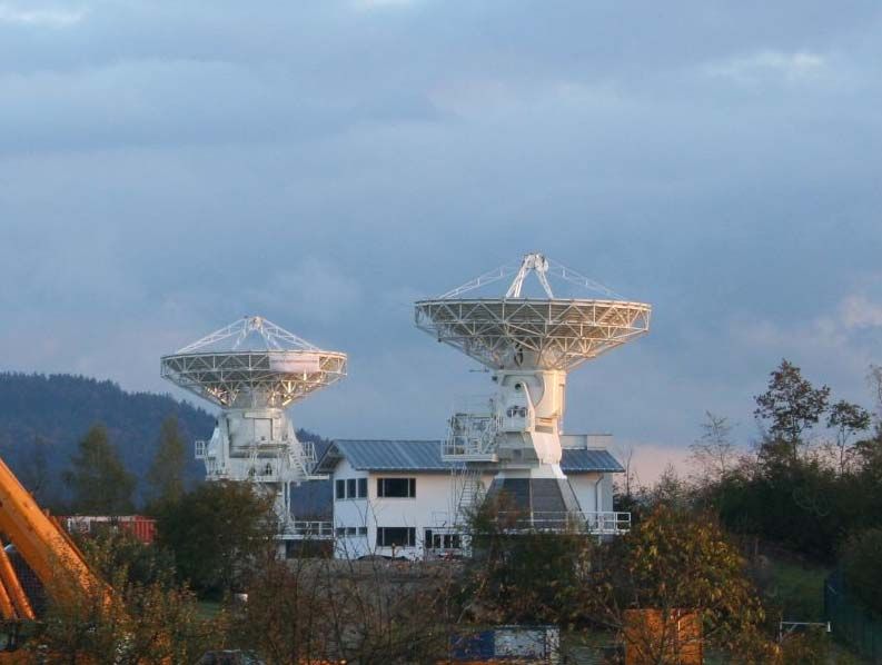
Shorter “on-source” timeFor VLBI2010 need faster slewing antennas
Smaller diameter: ~12-m; >50% efficient
12°/s azimuth rate; 6°/s elevation rate
Pictured here:
Twin Telescopes Wettzell (Vertex)
Other antennas meeting spec include:
• MT Mechatronics - RAEGE project (Spain & Portugal)
• IntertronicsNeed short on-source times
“Burst Mode”
Acquire data at
32 Gbps while on-source
Use extremely
high data and
record rates Record data at
8 Gbps while slewing
Short between sources
on-source
time
Use Broadband Broadband feeds
Delay (BBD) 2-14 GHz
**NEW**
Resolve phase
delay at Four 1-GHz bands
modest SNR across 2-14 GHzVLBI2010 System Block Diagram
Complete redesign relative to legacy S/X system
Antenna
Cryostat Control Room
V-pol LNA
Flexible
RF over Down- Rcd/
fibre DBE
LNA converter BW=1GHz eVLBI
H-pol 2-14 GHz 8 Gbps
HV-pol
BW=1GHz ‘burst’
HV-pol
PCAL
Generator Stable
cable
H-maser
LMR-400Haystack Approach
Antenna
Cryostat Control Room
V-pol LNA
RF over UDC
fibre 2-12 GHz RDBE MK6/
LNA
H-pol BW=512MHz BW=512MHz Mk5C
HV-pol HV-pol
PCAL
Generator Stable
cable
H-maser
LMR-400
DBBC Approach
Antenna Control Room
Cryostat
V-pol LNA DBBC3 Digital over DBBC
fibre MK6/
28 Gsps VLBI Mk5C
8-bit 2010
LNA
H-pol
Stable cable
H-maser
LMR-400Broadband Delay requires separation of
dispersive and non-dispersive delay
during (not after) fringe detection
Non-dispersive delay.
Delay is independent
of frequency (phase
is linear wrt frequency)
Combination
Phase (cycles)
φ = f ⋅τ
Non-dispersive φ = f ⋅ (τ g + τ clk + τ atm + ...)
component
Dispersive
Dispersive delay.
Delay varies with
component
frequency. Variation is
due to the Ionosphere.
K K
0 2 4 6 8 10 12 14 16 φIon = τ Ion = −
f f2
Frequency (GHz)Level 1 Solution: Group Delay only
Example optimized sequence
11.7 GHz
2.5 GHz
7.1 GHz
4.9 GHz
Phase (cycles)
With SNR=10 per band and a group delay
only solution, ΔƬ=~32 ps (~1 cm).
0 2 4 6 8 10 12 14 16
Frequency (GHz)Level 2 solution: Using the group delay
solution, connect the phase between bands
Need to resolve integer cycles of phase between bands
For SNR=10 per band and
phase resolved between all
bands, Δτ=~5-ps (~2 mm).
0 2 4 6 8 10 12 14 16Level 3 solution: Using the connected phase
solution, resolve the phase offset
Phase (cycles)
For SNR=10 and the phase offset resolved,
Δτ = ~1.3 ps (~0.5 mm).
0 2 4 6 8 10 12 14 16
Frequency (GHz)In practice, a search algorithm is used
to determine Ƭ and K
Phase (cycles)
Observed Non-dispersive
φ = f ⋅τ Search to find values
of Ƭ and K that flatten
K the observed delay
Dispersive φ= (when subtracted) and
f
hence maximize the
coherent sum
0 2 4 6 8 10 12 14 16
Frequency (GHz)VLBI works best with circular polarization
As seen from above, the linear polarization orientation for alt/az
antennas varies with geographic location
1 2 3 4 5
3 * 3 1 * 3
For parallel orientations, For orthogonal orientations,
correlated signal is found correlated signal shifts
in the co-pol products, to the cross-pol products
e.g. v1*v2 and h1*h2 e.g. v1*h2 and h1*v2
To avoid the shifting of correlated amplitude between cross- and co-pol products ,
VLBI traditionally uses circular polarization, where correlated amplitude is
independent of relative polarization orientation.
Although unprecedented, VLBI2010 uses linear polarizations directly. All four
polarization products are correlated and combined to generate a total intensity (I)
observable post-correlation. [Circular polarization could be generated electronically at
each antenna using 90°-hybrids but LNA imbalances are a problem.]Post-correlation determination of Total Intensity
( ) (
I = v1 ⋅ v2* + h1 ⋅ h2* ⋅ cos Δ + v1 ⋅ h2* − h1 ⋅ v2* ⋅ sin Δ )
φ1 φ2
Δ ~ differential antenna polarization angle, i.e. Δ = φ2 − φ1
Free air
Antenna Receiver Sampled output
signal
v Gv V = Gv ⋅ (v + Dh ⋅ h )
x-pol
coupling
h Gh H = Gh ⋅ (h + Dv ⋅ v )
Need to know G and D terms
- can be determined by observing a strong unpolarized point
source
- G terms can be tracked using noise and phase cal signalsVLBI2010 Antenna/Feed/Receiver Summary • Antenna Azimuth slew rate: 12°/s • Antenna Elevation slew rate: 6°/s • SEFD: < 2500 Jy • Frequency range: 2-14 GHz • Polarizations: V-pol, H-pol (linear) • # of bands: 4 • Bandwidth per band: 1 GHz • Data rate (burst): 16 Gbps (eventually 32 Gbps) • Sustained record rate: 8 Gbps (eventually 16 Gbps)
Resources, e.g.:
   • “Radio Astronomy Tutorial”,
   http://www.haystack.mit.edu/edu/undergrad/materials/RA_tutorial.html
   • “Essential Radio Astronomy”,
   http://www.cv.nrao.edu/course/astr534/ERA.shtm

Many thanks to Brian Corey for assistance with course material preparation!

           Questions?
You can also read