The partial response SVM - ESANN 2021
←
→
Page content transcription
If your browser does not render page correctly, please read the page content below
ESANN 2021 proceedings, European Symposium on Artificial Neural Networks, Computational Intelligence
and Machine Learning. Online event, 6-8 October 2021, i6doc.com publ., ISBN 978287587082-7.
Available from http://www.i6doc.com/en/.

                             The partial response SVM
                       B. Walters, S. Ortega-Martorell, I. Olier and P.J.G. Lisboa*

              Data Science Research Centre, School of Computer Science and Mathematics
               Liverpool John Moores University, Byrom Street, Liverpool L3 3AF, UK

           Abstract. We introduce a probabilistic algorithm for binary classification based on
           the SVM through the application of the ANOVA decomposition for multivariate
           functions to express the logit of the Platt estimate of the posterior probability as a
           non-redundant sum of functions of fewer variables (partial responses) followed by
           feature selection with the Lasso. The partial response SVM (prSVM) is compared
           with previous interpretable models of the SVM. Its accuracy and stability are
           demonstrated with real-world data sets.

     1    Introduction

     1.1 Motivation
     Black-box models are not interpretable by design, lacking transparency and
     accountability [1]. In particular for binary classification the SVM is a powerful
     discriminant model, but its deployment in high-stakes applications is limited by two
     factors: first, its roots in computational learning theory do not conform to the models
     of chance variation that are required to infer a posterior probability; second, the use of
     Gaussian makes it difficult to quantify the exact weight of each input towards the
     model output. As a consequence, the end user does not know for instance why
     specifically an SVM has misclassified for a particular example [2]. The first aspect
     has been the subject of extended research. Arguably the simplest approach to take is
     to use Platt’s approximation [3] by re-calibrating the decision function of the SVM
     i.e. the risk score function, by using a logistic regression model with parameters
     estimated by minimising the standard negative log-likelihood. We use this
     approximation but make the logistic regression model multivariate by applying it to
     multiple components derived from the decision function.
            Explanations for model decisions, however, can be pivotal in users making
     decisions e.g. in medical decision support [4]. There are several definitions of
     transparency and interpretability throughout the literature, but five main desiderata
     have been proposed for robust interpretability and explainability [5,6], that will guide
     the proposed approach: Intelligibility: “Are the explanations immediate and
     understandable?”; Faithfulness: “Are relevance scores indicative of ‘true’
     importance?”; Stability: “How consistent are the explanations for neighbouring
     examples?”; Parsimony: “Do the explanatory variables comprise a minimal set?”; and
     Consistency: “How robust are the explanations to perturbations in the data?”. In our
     view, an interpretable method that can fit these five criteria is the key to opening the
     black box corresponding to a standard l1-regularised SVM.

     *
       Bradley Walters would like to thank Liverpool John Moores University for
     a PhD Studentship

                                                    575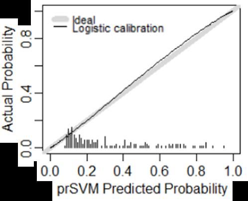
ESANN 2021 proceedings, European Symposium on Artificial Neural Networks, Computational Intelligence
and Machine Learning. Online event, 6-8 October 2021, i6doc.com publ., ISBN 978287587082-7.
Available from http://www.i6doc.com/en/.

           A key aim of the proposed approach is to create a method that focuses on
     contribution rather than attribution. In this context we refer to attribution as a signal
     fed back from the model output to the input for the purposes of quantifying the
     sensitivity of the former to the latter. This may be derived from a local tangent model,
     such as LIME [4] providing an explanation at a specific data point about which
     variables are most important. In contrast, we refer to interpretability as the calculation
     feedforward of the exact contribution of each input to the model output, similar to
     what is the case in Generalised Additive Models (GAM). In particular, we aim to
     provide global interpretability over the whole data space by quantifying how much
     each variable contributes to a prediction.

     1.2 Related work
     Early approaches to interpreting SVMs sought to express them with Boolean rules
     and by identifying prototypes through clustering [7]. Later, it was suggested to use
     GAMs to interpret different machine learning models [8]. This built on a very early
     proposal to structure the neural networks as self-explaining models [9] that cross-over
     between machine learning and conventional statistics. However, the central issue of
     the selection of relevance features in a statistically principled way. This is critical to
     the efficient estimation of an interpretable model, especially when two-way effects
     are considered.
           The proposed approach is closely related to the SVM nomogram [10,11] which
     followed a similar argument also with Platt’s approximation, by considering a Taylor
     expansion of the Gaussian kernels, followed by an iterative re-weighted SVM applied
     to the component functions generated by the Taylor expansion, in order to reduce the
     number of required functions and provide stability to the model.
           In fact, the expansion used in Van Belle’s papers [10,11] and in this manuscript
     to express the multivariate Gaussian kernel as a sum of functions of fewer variables
     has the form of an ANOVA decomposition, which is finite and exact if all terms are
     taken into account. That is to say, for a p-dimensional input, it is composed of 2p
     terms comprising a constant and effects of order 1, 2, …, p. The assumption made in
     both papers is that in many real-world applications the signal-to-noise level will
     render higher-order terms less relevant because they are very difficult to infer
     accurately.
           Therefore, there is potential for, and possibly even a performance advantage to
     be gained in making the decomposition of the complex multivariate kernel into
     simpler functions of fewer variables, which we call partial responses. This way, the
     coefficients of the partial functions, which we model for univariate and bivariate
     effects, can be explicitly estimated and further, by truncating the ANOVA expansion,
     the signal-to-noise ratio of the risk score functions can be improved by removing the
     higher-order, noisier terms, that are implicit in the original multivariate function.
           The SVM nomogram followed earlier work [12] in the framework of Functional
     Data Analysis (FDA). This involves setting specialised regularisation terms to
     implement sparsity and smoothness in the risk score function, by driving down its
     derivative in specific ways. This makes the method of particular interest to certain
     types of data with correlated inputs e.g. smooth spectra and time series.

                                                 576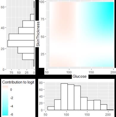
ESANN 2021 proceedings, European Symposium on Artificial Neural Networks, Computational Intelligence
and Machine Learning. Online event, 6-8 October 2021, i6doc.com publ., ISBN 978287587082-7.
Available from http://www.i6doc.com/en/.

     1.3 Novel contribution and limitations of this work
     The main contribution of this paper is an alternative methodology to calculate a
     nomogram for the SVM, by replacing the second SVM iteration in the model of [11]
     with the application of the logistic regression Lasso [13]. This has the advantage over
     the iterative re-weighted step of involving probabilistic modelling at the level of the
     partial responses including feature selection. This potentially improves calibration and
     stability in the selection of the final sparse model. It also simplifies the
     implementation of the SVM nomogram, so making it more easily accessible to other
     researchers.
           The main limitation of this work is that it applies only to tabular data,
     comprising independent covariates, as distinct from structured data such as images,
     speech and text.

     2         Methodology
     The implementation of the partial response SVM (prSVM) is straightforward:
          i.     Calculate the ANOVA decomposition to any desired order anchored at a
                 suitable point – we choose to use the median of data;
         ii.     Take the component functions, which are the partial responses at the anchor
                 point, to be the covariates in logistic regression Lasso.
           The first step is identical to the calculation of component functions in [10,11].
     The difference in this paper is the application of a probabilistic method directly to the
     partial responses, rather than to the score function arising from a linear SVM as the
     second step. This step involves aggressive pruning of the model coefficients, which
     required an iterative re-weighted algorithm where the regularisation parameters of the
     linear SVM were inversely proportional to the size of the corresponding model
     coefficients. Hence, the smaller the coefficient, the faster it would be pushed towards
     zero. Effective as this approach proved to be, it can be less stable than the Lasso. In
     addition, the availability of many coefficients for calibration, compared with a scalar
     risk score, makes it easier to achieve good calibration.
           It can be said that the prSVM utilises the benefits of the two models in a
     complementary way: the SVM contributes discriminant functions and the logistic
     Lasso carries out efficient feature selection.
           More formally, the partial responses are obtained from the logit of the Platt
     approximation to the probability of class membership, in other words directly from
     the risk score of the SVM, by evaluating it at the median of the data, then allowing
     one variable to change at a time, then two. The key is to formulate an orthogonal
     decomposition so that, for p-dimensional input data, the terms added up to
     interactions of order p exactly match the original function. The intention is to truncate
     this decomposition at order 2 as it is empirically observed that for many real-world
     applications e.g. in medicine, higher-order interactions seldom play a part in risk
     models, not least as low signal-to-noise ratios will make it difficult to infer such
     interactions accurately with reasonable sample sizes.
           The ANOVA decomposition anchored at the origin is defined by:

                                                 577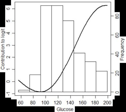
ESANN 2021 proceedings, European Symposium on Artificial Neural Networks, Computational Intelligence
and Machine Learning. Online event, 6-8 October 2021, i6doc.com publ., ISBN 978287587082-7.
Available from http://www.i6doc.com/en/.
(1)
where:
(2)
(3)
(4)
Having standardised the covariates to unit variance and shifted the origin to the
median, the values of the partial responses above for each row of data, become the
inputs to a standard logistic regression Lasso [13].
3 Empirical evaluation
3.1 Data description
The prSVM performance is compared with that of the original SVM with a Gaussian
kernel and the SVM nomogram model [11] using the same two real-world data sets.
The Pima diabetes dataset (n=532) comprises measurements from women aged
over 21 years old, of Pima Indian heritage, tested for diabetes. There are 7 covariates
and the binary outcome classes have a prevalence of 33.27%.
The German Credit Card dataset (n=1000) using the same 6 covariates as [11]
for comparability and outcomes of good or bad credit risk with a prevalence of 30%.
3.2 Classification performance
The two models for real-world data were optimised by 4-fold cross validation on the
training data. For both models the hyperparameter was tested in the range [2-7,22]
with the values 2-2 and 2-4 selected for the Pima and German Credit Card datasets
respectively.
The relative performance compared to the original SVM and the values quoted
in [11] are listed in Table 1. Note the smaller number of variables selected, for a
similar classification performance. This is important because smaller univariate and
bivariate effects are more difficult to infer accurately and can be unstable.
The implementation of SVM in R by [14] involves a cost parameter that
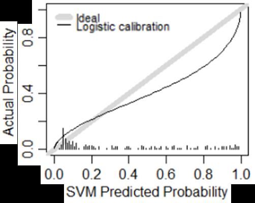
penalises misclassifications. The effect on calibration of both the hyperparameters
was considered and the calibration for the Pima dataset is shown in fig. 1. This is
consistent with the hypothesis that modelling the SVM with component functions
renders the prSVM a more accurate probabilistic model than resorting to the Platt
approximation. The form of the partial responses provides valuable insights about the
validity of the model predictions, as it can be verified by expert end-users.
578ESANN 2021 proceedings, European Symposium on Artificial Neural Networks, Computational Intelligence
and Machine Learning. Online event, 6-8 October 2021, i6doc.com publ., ISBN 978287587082-7.
Available from http://www.i6doc.com/en/.
Dataset Model AUC [CI] # H-L statistic
components (p-value)
PIMA SVM 0.801 [0.730,0.873] 7 26.5 (0.000867)
Diabetes prSVM 0.806 [0.737,0.876] 7 15.7 (0.0465)
SVM 0.780 28
Approx. [11]
German SVM 0.757 [0.696,0.818] 6 21.0 (0.00719)
Credit prSVM 0.754 [0.696,0.813] 18 11.2 (0.190)
Card SVM 0.760 21
Approx. [11]
Table 1: Results comparison between the original SVM, the prSVM and the SVM
Approximation in [11]. H-L stands for Hosmer-Lemeshow test statistic. The
#components is the #covariates for the SVM and the #partial responses for the rest.
Fig. 1: Calibration curves for the Pima diabetes data set, with hyperparameters =2-2
and Cost=10-2, showing an improvement for the prSVM compared with the original
SVM with a Gaussian kernel.
Fig. 2: Example partial responses in the nomogram for the Pima diabetes data set.
The contribution of each variable to the logit is shown on the y-axis. For a given
observation, these contributions add to form the nomogram. The responses show the
weights for Glucose and a 2-way interaction between Glucose and Skin thickness.
579ESANN 2021 proceedings, European Symposium on Artificial Neural Networks, Computational Intelligence
and Machine Learning. Online event, 6-8 October 2021, i6doc.com publ., ISBN 978287587082-7.
Available from http://www.i6doc.com/en/.
4 Conclusion
An alternative proposal for the calculation of the SVM nomogram is presented.
Compared with the original formulation in [11] the new approach is more stable to
generate sparse models. It shows markedly better calibration than the original SVM
while retaining a comparable classification performance.
A possible extension of this model is to calculate confidence intervals for the
partial responses by re-sampling with the bootstrap. This is particularly important for
quantifying uncertainty in underpopulated regions of the training data sample, shown
in the histograms along the axes in fig. 2.
References
[1] C. Rudin, Stop explaining black box machine learning models for high stakes decisions and use
interpretable models instead. Nature Machine Intelligence, 1:206-215, 2019.
[2] Y. Liang, S. Li, C. Yan, M. Li and C. Jiang, Explaining the black-box model: A survey of local
interpretation methods for deep neural networks. Neurocomputing, 419:168-182, 2021.
[3] J.C. Platt, Probabilistic Outputs for Support Vector Machines and Comparisons to Regularized
Likelihood Methods. In A.J. Smola, P. Bartlett, B. Schoelkopf, D. Schuurmans, editors, Advances in
large margin classifiers. Cambridge, MA, USA: MIT Press, pages. 61-74, 1999.
[4] M.T. Ribeiro, S. Singh and C. Guestrin, "Why should I trust you?" Explaining the predictions of any
classifier. In Proceedings of the 22nd ACM SIGKDD international conference on knowledge
discovery and data mining, pages 1135-1144, 2016.
[5] D. Alvarez-Melis and T.S. Jaakkola, Towards robust interpretability with self-explaining neural
networks. In Proceedings of the 32nd International Conference on Neural Information Processing
Systems (NIPS'18), pages 7786-7795, 2018.
[6] P.J.G Lisboa, S. Ortega-Martorell, M. Jayabalan and I. Olier, Efficient Estimation of General
Additive Neural Networks: A Case Study for CTG Data. In Joint European Conference on Machine
Learning and Knowledge Discovery in Databases, Springer, Cham, pages 432-446, 2020.
[7] H. Núñez, C. Angulo, and A. Català, Rule extraction from support vector machines. In Proceedings
of the European Symposium on Artificial Neural Networks (ESANN’02), pages 107–112, 2002.
[8] Y. Lou, R. Caruana, and J. Gehrke, Intelligible models for classification and regression.
In Proceedings of the 18th ACM SIGKDD International Conference on Knowledge Discovery and
Data Mining (KDD’12), ACM, pages 150–158, 2012.
[9] W.S. Sarle, Neural Networks and Statistical Models. In Proceedings of the Nineteenth Annual SAS
Users Group International Conference, 1994.
[10] V. Van Belle and P.J.G. Lisboa, White box radial basis function classifiers with component
selection for clinical prediction models. Artificial Intelligence in Medicine, 60:53-64, 2014.
[11] V. Van Belle, B. Van Calster, S. Van Huffel, J. Suykens and P. Lisboa, Explaining Support Vector
Machines: A Color Based Nomogram. PLOS ONE, 11(10), 2016.
[12] B. Martin-Barragan, R. Lillo and J. Romo, Interpretable support vector machines for functional data.
European Journal of Operational Research, 232:146-155, 2012.
[13] L. Meier, S. Van De Geer and P. Bühlmann, The group lasso for logistic regression. Journal of the
Royal Statistical Society: Series B (Statistical Methodology), 70:53-71, 2008.
[14] A. Karatzoglou, D. Meyer, K. Hornik, Support Vector Machines in R. Journal of Statistical
Software, 15:1-28, 2006.
580You can also read