Thermal Gradients on Planetary Bodies and the Molar Mass Ideal Gas Law
←
→
Page content transcription
If your browser does not render page correctly, please read the page content below
Thermal Gradients on Planetary Bodies and the Molar Mass Ideal Gas Law
   Robert IH*
   Faculty of Science and Engineering, Federation University, Mt Helen, Ballarat, Australia

   *
       Corresponding author: Robert IH, Faculty of Science and Engineering, Federation University, Mt Helen, Ballarat,
   Australia, Tel: 61418352801; E-mail: robertholmes@students.federation.edu.au

   Received: October 20, 2017; Accepted: February 08, 2018; Published: February 10, 2018

Abstract
It has always been complicated mathematically, to calculate the average near surface atmospheric temperature on planetary bodies with a
thick atmosphere. Usually, the Stefan Boltzmann (S-B) black body law is used to provide the effective temperature, then debate arises about
the size or relevance of additional complicating factors, including the albedo and the greenhouse effect. Presented here is a simple and reliable
method of accurately calculating the average near surface atmospheric temperature on planetary bodies which possess a surface atmospheric
pressure of over 10 KPa. The formula used is the molar mass version of the ideal gas law. This method requires a gas constant and the
measurement of only three gas parameters; the average near-surface atmospheric pressure, the average near surface atmospheric density
and the average mean molar mass of the near-surface atmosphere. This indicates that all information on the effective plus the residual near-
surface atmospheric temperature on planetary bodies with thick atmospheres, is automatically ‘baked-in’ to the three mentioned gas
parameters. It is known that whenever an atmospheric pressure exceeds 10 KPa, convection then dominates over radiative interactions as the
main method of energy transfer, and a rising thermal gradient is formed. This rising thermal gradient continues on down, (if there is a
depression or a mine shaft) to even below the average surface level. Given this thermodynamic situation, it is very likely that no one gas has
an anomalous effect on atmospheric temperatures that is significantly more than any other gas. In short; there is unlikely to be any
significant warming from the greenhouse effect on any planetary body in the parts of atmospheres which are >10 KPa. Instead, it is proposed
that the residual temperature difference between the S-B effective temperature and a measured near-surface temperature (the atmospheric
effect) is a thermal enhancement which is actually caused by auto-compression.

Keywords: Greenhouse effect; Temperatures of planets; Earth temperature; Venus temperature; Auto-C; Climate sensitivity; Global climate
change; Global warming; Atmospheric thermal gradient

   Introduction
   It is a postulate of this work that any warming effects arising from atmospheric greenhouse gases such as CO₂, are subjected
   to a 100% rate of negative feedbacks which are inherent in the climate system. The detail of these feedbacks will not be

   Citation: Robert IH. Thermal Gradients on Planetary Bodies and the Molar Mass Ideal Gas Law. J Phys Astron. 2018; 6(1):134
   © 2017 Trade Science Inc.                                                                                                            1
www.tsijournals.com | January-2018
outlined here, but the open nature of the atmosphere, coupled with the following thermodynamic arguments, indicate that this
postulate makes sense.
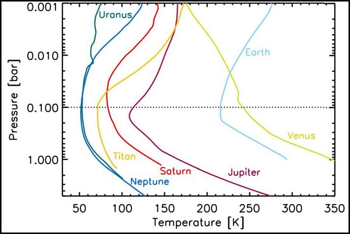
It is known that planetary bodies which have thick atmospheres, naturally set up a rising thermal gradient in that part of the
atmosphere which is higher than a pressure of 10 KPa, (0.1bar) until that bodies’ surface is reached [1] FIG. 1. Less well
known is that this rising temperature gradient continues even below the surface [2] making it difficult to attribute to the
greenhouse effect. In this denser part of the atmosphere, (on Earth, the troposphere) convection and adiabatic auto-
compression effects rule over radiative or ‘greenhouse’ effects in the determination of atmospheric temperatures and the
thermal gradient. However, higher up in the atmosphere, once the atmospheric pressure drops below 10 KPa (0.1 bar) then
radiative effects dominate. This is because the atmosphere there is too thin to initiate convection or any warming due to auto-
compression. Although the term ‘auto-compression’ may be unfamiliar to some, this can be seen as simply an engineering
term for what meteorologists call the ‘lapse rate’ and in astronomy is called the ‘Kelvin-Helmholtz’ contraction. Under the
latter, the contraction and so compression of a large inter-stellar molecular gas cloud under gravity, achieves such high
temperatures that nuclear fusion initiates, and a star is born [3].
FIG 1. A thermal gradient appears in all planetary atmospheres >10 KPa (0.1 bar) [1]
Using this knowledge, an exacting yet simple method is introduced, which enables the average near-surface atmospheric
temperature of any planetary body with an atmospheric pressure of over 10 KPa, to become easily and quickly calculated. A
molar version of the ideal gas law is utilised formulas 5 and 6, which consists of one gas constant and three basic atmospheric
gas parameters; the average near-surface atmospheric pressure, the average near-surface atmospheric density and the mean
molar mass of the near-surface atmosphere.
This formula proves itself here, to be not only more accurate than any other method heretofore used, but is far simpler to
calculate. It requires no input from parameters previously thought to be essential for the calculation of atmospheric
temperatures; for example, solar insolation, albedo, greenhouse gas content, ocean circulation and cloud cover among many
others. The reason these are not required, is because they, (and all others) are already automatically ‘baked-in’ to the three
2www.tsijournals.com | January-2018
gas parameters mentioned. Note: although terms for insolation intensity and auto-compression are not used in the formula, it
is proposed that these two are still what virtually determine the average near-surface planetary atmospheric temperature.
Venus is the planet which has been hard to explain
There has always been difficulty in explaining, or in formulating a simple method to satisfactorily explain or calculate the
very high surface atmospheric temperature of the planet Venus using conventional mathematical means or by employing the
greenhouse gas hypothesis. Here, the molar mass version of the ideal gas law will be used to simply and accurately determine
the surface temperature of this planet, by the measurement of just three variable gas parameters and the knowledge of one
fixed gas constant.
Molar mass version of ideal gas law calculates planetary surface temperatures
The ideal gas law may be used to more accurately determine surface temperatures of planets with thick atmospheres than the
S-B black body law [4], if a density term is added; and if kg/m³ is used for density instead of gms/m³, the volume term V may
be dropped. This formula then may be known as the molar mass version of the ideal gas law.
The ideal gas law is; PV = nRT (1)
Convert to molar mass; PV = m/M.RT (2)
Convert to density; PM/RT = m/V = ρ (3)
Drop the volume term; ρ = P/(R.T/M) (4)
P
Find for temperature; T (5)
R
M
V= Volume
m= Mass
n= Number of moles
T= Near-surface atmospheric temperature in Kelvin
P= Near-surface atmospheric pressure in KPa
R= Gas constant (m³, KPa, Kelvin⁻¹, mol⁻¹) = 8.314
ρ= Near-surface atmospheric density in kg/m³
M= Near-surface atmospheric mean molar mass (gm/mol⁻¹)
Alternatively, the molar mass version of the ideal gas law can be written thus
T PM (6)
R
Methodology involves calculating average near-surface temperature of planets
Formula 5 is here used throughout.
Using the properties of Venus [5],
3www.tsijournals.com | January-2018
9200
T
65
8.314
43.45
Venus calculated surface temperature = 739.7K
Using the properties of Earth from Wiki, [6]
101.3
T
1.225
8.314
28.97
Earth calculated surface temperature = 288.14K
Venus is calculated at 739.7K, which is given by NASA as ~740K. Earth is calculated at 288K, currently its quoted by
NASA [7] at 288K. It will be noted that the average temperature of the surface of Titan was measured by the Voyager 1, and
by the Huygens lander [8] and was probably used as an input to find the surface density; (the independently-measured surface
density on Titan could not be found in the literature). The 94K will therefore come out of the below formula, since it is a
rearrangement of formula 1. This could be seen as a circular argument. However, it is unlikely that if and when the density of
Titan is directly measured, for instance by the use of a dasymeter or similar, it will be significantly different from the
5.25kg/m³ stated here.
Calculate for Titan, data [9];
146.7
T
5.25
8.314
28.0
Titan calculated surface temperature = 93.6K
Calculate for Earth’s South Pole, data [10];
68.13
T
1.06
8.314
28.97
Earth’s South Pole average calculated temperature = 224K (-49°C) Calculate for Mars;
0.69 0.9
T T
0.02 0.02
8.314 8.314
43.34 43.34
Mars calculated surface temperature = 180K to 234K
The average temperature on Mars is 210K; as suspected from other work [1] this method is inaccurate for Mars, due to the
very low and variable atmospheric pressure. Pressures here were measured at the Viking 1 landing site and varied between
690Pa and 900Pa according to the season. It is only in atmospheres with a pressure of over 10 KPa (0.1bar) that strong
convection and a troposphere/tropopause is formed, and its associated thermal gradient. Mars is included to demonstrate the
4www.tsijournals.com | January-2018
validity of the >10 KPa rule. For Mars, the mid-point between the summer and the winter pressures is used, which results in a
temperature of 207K. The gas giants will now be assessed; note that these planets do not have a defined surface like the
terrestrials planets have, so here they are given a ‘surface’ by using the Earth’s surface pressure of 101.3 KPa (1 atm) as a
level to use for this calculation.
Calculate for Jupiter [7];
101.3
T
0.16
8.314
2.2
Jupiter calculated temperature at 1atm of pressure = 167K
Calculate for Saturn [7];
101.3
T
0.19
8.314
2.07
Saturn calculated temperature at 1atm of pressure = 132.8K
Calculate for Uranus [7];
101.3
T
0.420
8.314
2.64
Uranus calculated temperature at 1atm of pressure = 76.6K
Calculate for Neptune [7];
101.3 101.3
T T
0.450 0.450
8.314 8.314
2.53 2.69
In the case of Neptune, NASA gave two values for mean molar mass; 2.53 and 2.69, this necessitated two separate
calculations to give a high and a low of calculated temperatures. Neptune’s calculated temperature at 1atm of pressure =
68.5K to 72.8K. The temperature on Neptune at 1atm of pressure is 72K; this lies quite between the two calculated
temperatures (TABLE 1).
TABLE 1. Comparison of calculated and actual average surface temperatures.
Planetary body Calculated temperature Kelvin Actual temperature Kelvin Error
Venus 739.7 740 0.04%
Earth 288.14 288 0.00%
South Pole of Earth 224 224.5 0.20%
Titan 93.6 94 0.42%
Mars (low pressure) 180 to 234 210 1.40%
Jupiter 167 165 1.20%
Saturn 132.8 134 0.89%
Uranus 76.6 76 0.79%
Neptune 68.5 to 72.8 72 0.00%
5www.tsijournals.com | January-2018
Analysis about the postulate and hypothesis being presented herein
If this simple relationship between surface atmospheric density, pressure and molar mass is an accurate method of predicting
surface temperatures on bodies with a thick atmosphere, it will necessarily be informative about what actually determines
these planetary surface temperatures, and will have important implications for climate sensitivity.
In short, a postulate being put forward here, is that in the case of Earth, solar insolation provides the ‘first’ 255 Kelvin – in
accordance with the black body law [11]; this being the ‘effective’ or the ‘base’ level. Then gravitationally induced auto-
compression provides the ‘other’ 33 Kelvin, termed the ‘residual’, to arrive at the known and measured average global
temperature of 288 Kelvin. The ‘other’ 33 Kelvin is not hypothesised to be provided by the greenhouse effect, because if it
was, the molar mass version of the ideal gas law would not then work to accurately calculate real planetary temperatures in
the case of small incremental changes to gas levels, as it clearly does here.
Temperature in a gas is a measure of the average kinetic energy of the particles in the gas. When atmospheric gas pressure
exceeds 10 KPa, a temperature gradient is set up from that pressure level [1], down to the planetary surface (this thermal
gradient is known and measured to continue even below the surface, if there is for example, a mine shaft). It is postulated
here, that the cause of this thermal gradient is gravity-induced auto-compression. In general terms, the surface temperature
sets up convective overturning of the troposphere, which is adiabatic through much of the convection cycle [2], and this
combines with gravitationally induced atmospheric auto-compression to create the observed tropospheric thermal
enhancement and temperature gradient.
The origins of this thermal effect on gases go back to James Maxwell, who, in his 1872 book ‘Theory of Heat’ [12]
demonstrated that the formation of the thermal gradient from the tropopause downwards is assisted by convection and more
particularly, the increasing atmospheric pressure, which itself is a result of a combination of the Earth’s gravitational field
and the atmospheric density.
“In the convective equilibrium of temperature, the absolute temperature is proportional to the pressure.” [12].
The idea of a thermal gradient naturally forming in any column of gas in a gravitational field was first proposed in the 1860’s
by Loschmidt [13]. At the time, Maxwell thought that this idea violated the second law of thermodynamics, yet as has been
shown here, derivations of Maxwell’s own ideal gas law is an excellent predictor of temperatures – when the atmosphere is
thick enough to be compressed by a gravitational field.
The controversy between Loschmidt on one side, with Maxwell and Boltzmann on the other, raged for some time and was
finally experimentally tested in 2007, with the results published by Graeff [14]. Graeff’s experiments concluded that a
gravitationally-induced temperature gradient does spontaneously develop in sealed columns of both air and water – the
bottom of the column being warmer than the top. The theoretical amounts of warming according to Graeff should be 0.07K/m
and 0.04 K/m respectively. Graeff’s experimental apparatus reported 0.07K/m and 0.05K/m – so basically confirming
6www.tsijournals.com | January-2018
Loschmidt’s predictions. The thermal gradient appeared, despite the reverse gradient being prevalent in the immediate
environment of the experiment. Loschmidt originally has said that the second law of thermodynamics needed to be re-stated
to include the effects of gravitational fields on fluids.
The adiabatic auto-compression hypothesis enunciated herein, states that convection/pressure/lapse rate effects dominate over
radiative effects in regions of all planetary atmospheres >0.1 bar and a temperature gradient is naturally formed. In effect,
gravity formes a density and a temperature gradient; pressure is a corollary.
Auto-compression is known and used daily in mining
Auto-compression is well known in underground mining, and is used by ventilation engineers to calculate how hot the mine
air will get, so that they know how much cooling air to provide at each level. The effect of auto-compression can be
calculated by the following relationship;
Pe = Ps exp(gH/RT)
Where;
Pe = Absolute pressure at end of column (KPa)
Ps = Absolute pressure at start of column (KPa)
g = Acceleration due to gravity (m/s²)
H = Vertical depth (m)
As can be clearly seen, this effect primarily relies on pressure and gravity, which will be different for each planetary body.
Mechanism is adiabatic
Note that we are examining an adiabatic process, and when a gas parcel expands adiabatically, as it does when rising in a
gravitational field, it does positive work – and the kinetic energy drops and so the temperature drops. However, when a gas
parcel is compressed, as it is when is descends in a gravitational field, then it does negative work, and its kinetic energy rises
and so its temperature goes up. Why does the kinetic energy of the gas rise when descending? It’s because some of its
potential energy is converted to enthalpy, so producing an increase in pressure, specific internal energy and hence,
temperature in accordance with the following equation;
H = PV + U
Where;
H = Enthalpy (J/kg)
P = Pressure (Pa)
V = Specific volume (m³)
U = Specific internal energy (kinetic energy)
Discussion on Maxwell vs. Arrhenius and the ‘Greenhouse effect’
Work in this area of gas physics was detailed in the 19th century. However, there is a strong difference between the work and
the views of the researchers Maxwell and Arrhenius. Maxwell’s work shows that temperatures in the lower troposphere of
Earth are primarily determined by convection and the atmospheric mass/pressure/gravity relationship. Arrhenius’s later work
7www.tsijournals.com | January-2018
[15] completely ignored this and determined that temperatures in the lower troposphere of Earth are caused by the radiative
effects of greenhouse gases. There have been papers critical of Arrhenius’s radiative effects ideas since 1909 [16]. Who is
correct is critical to the present, since if Arrhenius is correct, then there should be some concern about CO₂ emissions, if the
climate sensitivity is high enough. If Loschmidt’s version of Maxwell’s work is correct, then more CO₂ will have no
measurable effect on tropospheric atmospheric temperatures.
What do atmospheric measurements actually show? Measurements [17] of the effects of more CO₂ in the atmosphere appear
to strongly support Maxwell. At pressures above 0.1 bar, “the extra CO₂ merely replaces water vapour” and little difference
is seen in temperatures – but at pressures below 0.1 bar more CO₂ is measured to cause strong cooling. One of the main
problems with the Arrhenius view, appears to be that convection is virtually ignored as a mode of heat transfer; later work
shows that only 11% of heat transfer in the troposphere is actually carried by radiation [18]. Whether this can cause
significant net warming in an open atmosphere is debatable. A recent paper has supported the Arrhenius view somewhat by
quantifying a forcing due to increased atmospheric CO₂ [19]. But there remains a lack of any paper in the literature, which
quantifies any warming attributable to increasing atmospheric CO₂ concentrations.
The accuracy and implications of formulas 5 and 6
It is apparent that this simple formula calculates the ‘surface’ temperatures of many planetary bodies in our Solar System
accurately FIG 2. Specifically, those which have atmospheres thick enough to form a troposphere (i.e. possessing an
atmospheric pressure of over 10 KPa or 0.1bar). These are; Venus, Earth, Jupiter, Saturn, Titan, Uranus and Neptune. All
calculated temperatures are within 1.2% of the NASA reported ‘surface’ temperature (except for Mars, which is excluded
because it has a much lower atmospheric pressure than 10 KPa). This accuracy is achieved without using the S-B black body
law, or the need to include terms for such parameters as TSI levels, albedo, clouds, greenhouse effect or, for that matter,
adiabatic auto-compression. All that is required to be able to accurately calculate the average near-surface atmospheric
temperature, is the relevant gas constant and the knowledge of three variable gas parameters.
FIG. 2. Actual temperature vs. calculated temperature of 8 planetary bodies and the South Pole
8www.tsijournals.com | January-2018
Discussion on the implications for climate sensitivity to CO₂
The reporting of climate sensitivity in the literature has been steadily reducing for decades, with some recent papers pointing
to a very low sensitivity, of much less than 1°C [20-22]. A careful reading of these papers, (for example the most recent one)
clearly indicates that the 0.6°C cited, is in fact an absolute maximum. This present work, if not invalidated by subsequent
work, clearly points to a climate sensitivity so low that it would not be possible to measure it in the real atmosphere; it could
even be negative (i.e., more CO₂ creates cooling). This work leads directly to the conclusion that a small change in any single
atmospheric gas, such as a doubling of the CO₂ level, (from the so-called ‘pre-industrial’ 0.03% to 0.06%) can have no
measurable positive or negative effect on atmospheric temperatures.
Probable implications for the climate sensitivity to CO₂
Some reflection upon the simplicity and accuracy of these results, combined with knowledge of significant other factors such
as the thermal gradient, should bring an unbiased person to some probable implications of this work. These are that the
residual near-surface atmospheric temperatures on planetary bodies with thick atmospheres are not mainly determined by the
greenhouse effect, but instead most likely by an effect from fluid dynamics, namely; auto-compression. This leads directly to
the conclusion that the climate sensitivity to, for example, a doubling of the atmospheric carbon dioxide concentration has to
be not only operating instantaneously, but also must be extremely low. Under this scenario, logic spells out that the
temperature change caused by the addition of 0.03% of CO₂ in the lower troposphere, cannot be very different to the addition
of a similar quantity of any other gas.
To be clear, formulas 5 and 6 appear to rule out any possibility that 33°C of global warming from a ‘greenhouse effect’ of the
type proposed by the IPCC in their reports [23] can exist in the real atmosphere. The reason is that the IPCC state in their
reports that a 0.03% increase in atmospheric CO₂, which represents a doubling from pre-industrial levels, must result in a
global lower tropospheric near-surface temperature rise of ~3°C; (within a range of 1.5°C to 4.5°C) [24,25] and an even
greater temperature rise in the upper troposphere.
This reported level of climate sensitivity to a doubling of atmospheric CO₂, has not changed significantly in the regular IPCC
reports since 1990. Anything like this magnitude of warming caused by such a small change in gas levels appears to be
completely ruled out by the molar mass version of the ideal gas law. The reason is that inserting any reasonable changes to
the three gas paraments caused by the small 0.03% of extra CO₂ into the formula, leads to almost no change in atmospheric
temperatures. A reasonable expectation would be that a 0.03% increase in atmospheric CO₂, which is a relatively heavy gas,
would result in the following changes in the three gas parameters;
Pressure: An increase of 0.03%
Density: An increase of 0.05%
Molar Mass: An increase of 0.05%
Calculate for a doubling of CO₂ from the pre-industrial level of 0.03% (by volume);
9www.tsijournals.com | January-2018
101.33
T
1.2256
8.314
28.984
Calculated temperature after doubling of CO₂ to 0.06% ≈ 288.23K
Climate sensitivity to CO₂ ≈ 288.23 - 288.14 ≈ 0.09K
The change would in fact be extremely small and difficult to estimate exactly, but would be of the order 0.09°C. That is,
thirty-three times smaller than the stated ‘likely’ climate sensitivity of 3°C cited in the IPCC’s reports. Even that small
number would likely be a maximum change, since if fossil fuels are burned to create the emitted CO₂, then atmospheric O₂
will also be consumed, reducing that gas in the atmosphere – and offsetting any temperature change generated by the extra
CO₂. This climate sensitivity is already so low that it would be impossible to detect or measure in the real atmosphere, even
before any allowance is made for the consumption of atmospheric O₂.
Conclusion
It has always been complicated mathematically, to calculate the average near surface atmospheric temperature on planetary
bodies with a thick atmosphere. Usually, the (S-B) black body law is used to provide the effective temperature, then debate
arises about the size or relevance of additional factors such as the greenhouse effect. Here is presented a simple and reliable
method of calculating the average near surface atmospheric temperature on planetary bodies which possess a surface
atmospheric pressure of over 10 KPa. This method requires knowledge of the gas constant and the measurement of only three
atmospheric gas parameters; average near- surface atmospheric pressure, average near surface atmospheric density and the
mean molar mass of the atmosphere.
The formula used is the molar mass version of the ideal gas law. It is here demonstrated that the information contained in just
these three gas parameters alone is an extremely accurate predictor of average near-surface atmospheric temperatures, in
atmospheres >10 KPa. Therefore, all information on the effective plus the residual near-surface atmospheric temperature on
planetary bodies with thick atmospheres; residual meaning the difference between the effective, (that predicted by S-B black
body law), and the measured actuality, must be automatically ‘baked-in’ to the three mentioned gas parameters.
This leads directly to the conclusion that a small change in any single atmospheric gas, not only has little effect on
atmospheric temperatures, but has a very similar effect to the same percentage change in any other atmospheric gas. It is seen
therefore, that no one gas particularly affects atmospheric temperatures more than any other gas; so, there can be no
significant ‘greenhouse warming’ caused by ‘greenhouse gases’ on Earth, or for that matter on any other planetary body.
Instead, it is hypothesised that the residual temperature differences, and the tropospheric thermal gradient observed on
planetary bodies, are actually caused by auto-compression.
10www.tsijournals.com | January-2018
Acknowledgement and Funding
Acknowledgement of non-specific Australian government support through “The Australian Government Research Training
Program Scholarship”.
REFERENCES
1. Robinson TD, Catling DC. Common 0.1 bar tropopause in thick atmospheres set by pressure-dependent infrared
transparency. Nature Geoscience. 2014; 7:12-15.
2. McPherson MJ. Subsurface ventilation and environmental engineering: Springer Science & Business Media.
2012.
3. Elmegreen BG, Elmegreen DM. Do density waves trigger star formation. The Astrophysical Journal. 1986;
311:554-62.
4. Stefan J. On the relationship between thermal radiation and temperature. Bulletin from the sessions of the
Vienna Academy of Sciences. 1879; 79:391-28.
5. Zasova LV, Ignatiev N, Khatuntsev I, et al. Structure of the Venus atmosphere. Planetary and Space Science.
2007; 55:1712-1728.
6. Wikipedia Properties of Earth’s atmosphere. Accessed. 2017.
https://en.wikipedia.org/wiki/Atmosphere_of_Earth
7. NASA fact sheet data on the planets. 2017.
8. Fulchignoni M, Ferri F, Angrilli F, et al. In situ measurements of the physical characteristics of Titan's
environment. Nature. 2005; 438: 785-91.
9. Lindal GF, Wood G, Hotz H, et al. The atmosphere of Titan: An analysis of the Voyager 1 radio occultation
measurements. Icarus. 1983; 53:348-63.
10. IceCube Wise. Wis/Mad Uni. 2017
11. NASA. Black body curves Sun and Earth. 2017
12. Maxwell JC. Theory of heat. Courier Corporation. 2012.
13. Flamm D. Four papers by Loschmidt on the state of thermal equilibrium. Pioneering ideas for the physical and
chemical sciences. Springer. 1997; 199-202
14. Graeff RW. Viewing the controversy Loschmidt–Boltzmann/Maxwell through macroscopic measurements of
the temperature gradients in vertical columns of water. Preprint. Additional Results Are on the Web Page. 2007
15. Arrhenius S. On the influence of carbonic acid in the air upon the temperature of the ground. The London,
Edinburgh, and Dublin Philosophical Magazine and Journal of Science. 1896; 41:237-76.
16. Wood RW. Note on the theory of the greenhouse. The London Edinburgh and Dublin Philosophical Magazine
and Journal of Science. 1909; 17:319-20.
17. Clough SA, Iacono MJ, Moncet JL. Line‐by‐line calculations of atmospheric fluxes and cooling rates:
Application to water vapor. Journal of Geophysical Research: Atmospheres. 1992; 97:15761-785.
18. Khilyuk L. Global warming: are we confusing cause and effect? Energy Sources. 2003; 25:357-70.
19. Feldman DR, Collins WD, Gero PJ, et al. Observational determination of surface radiative forcing by CO₂ from
2000 to 2010. Nature. 2015; 519:339-43.
11www.tsijournals.com | January-2018
20. Harde H. Advanced two-layer climate model for the assessment of global warming by CO₂. 2014.
21. Cederlof M. Using seasonal variations to estimate earth's response to radiative forcing. 2014.
22. Abbot J, Marohasy J. The application of machine learning for evaluating anthropogenic versus natural climate
change. GeoResJ. 2017; 14:36-6.
23. Team CW, Pachauri R, Meyer L. IPCC: Climate Change 2014: Synthesis Report. Contribution of Working
Groups I. II and III to the Fifth Assessment Report of the Intergovernmental Panel on Climate Change. 2014;
151.
24. Allen MR, Barros VR, Broome J, et al. IPCC Fifth Assessment Synthesis Report-Climate Change. Synthesis
Report. 2014.
25. Hess SL, Henry RM, Leovy CB, et al. Meteorological results from the surface of Mars: Viking 1 and 2. Journal
of Geophysical Research. 1977; 82:4559-74.
12You can also read