THOMAS RIDDICK 245 2021 - MPG.PURE
←
→
Page content transcription
If your browser does not render page correctly, please read the page content below
Generation of HD Parameters Files for ICON Grids
                  - Technical Note -

                 Thomas Riddick
                   Hamburg 2021

Berichte zur Erdsystemforschung                  245
Reports on Earth System Science                 2021
Hinweis                                          Notice
Die Berichte zur Erdsystemforschung werden       The Reports on Earth System Science are
vom Max-Planck-Institut für Meteorologie in      published by the Max Planck Institute for
Hamburg in unregelmäßiger Abfolge heraus-        Meteorology in Hamburg. They appear in
gegeben.                                         irregular intervals.

Sie enthalten wissenschaftliche und technische   They contain scientific and technical contribu-
Beiträge, inklusive Dissertationen.              tions, including Ph. D. theses.

Die Beiträge geben nicht notwendigerweise die    The Reports do not necessarily reflect the
Auffassung des Instituts wieder.                 opinion of the Institute.

Die "Berichte zur Erdsystemforschung" führen     The "Reports on Earth System Science" continue
die vorherigen Reihen "Reports" und "Examens-    the former "Reports" and "Examensarbeiten" of
arbeiten" weiter.                                the Max Planck Institute.

Anschrift / Address                              Layout
Max-Planck-Institut für Meteorologie             Bettina Diallo and Norbert P. Noreiks
Bundesstrasse 53                                 Communication
20146 Hamburg
Deutschland
                                                 Copyright
Tel./Phone: +49 (0)40 4 11 73 - 0
Fax:        +49 (0)40 4 11 73 - 298              Photos below: ©MPI-M
                                                 Photos on the back from left to right:
name.surname@mpimet.mpg.de
                                                 Christian Klepp, Jochem Marotzke,
www.mpimet.mpg.de
                                                 Christian Klepp, Clotilde Dubois,
                                                 Christian Klepp, Katsumasa Tanaka
Generation of HD Parameters Files for ICON Grids
                - Technical Note -

               Thomas Riddick
                 Hamburg 2021
Thomas Riddick

Max-Planck-Institut für Meteorologie
Bundesstrasse 53
20146 Hamburg

Berichte zur Erdsystemforschung / Max-Planck-Institut für Meteorologie    245
Reports on Earth System Science / Max Planck Institute for Meteorology   2021

ISSN 1614-1199

Technical Note: Generation of HD Parameters Files for
                        ICON Grids
                                        Thomas Riddick
                                        7th August 2021

Contents
1 Introduction                                                                                                              3
  1.1 Introduction . . . . . . . . . . . . . . . . . . . . . . . . . . . . . . . . . . . . . . .                            3
  1.2 Acknowledgements . . . . . . . . . . . . . . . . . . . . . . . . . . . . . . . . . . .                                3

2 Methods for Generating ICON River Directions and Parameters                                                                5
  2.1 General Notes . . . . . . . . . . . . . . . . . . . . . . . . . . . . . . .               .   .   .   .   .   .   .    5
  2.2 Procedure for Low Resolutions Without Internal Sinks . . . . . . . .                      .   .   .   .   .   .   .    6
  2.3 Procedure for Low Resolutions With Internal Sinks . . . . . . . . . .                     .   .   .   .   .   .   .   11
  2.4 Procedure for High Resolutions Without Internal Sinks . . . . . . . .                     .   .   .   .   .   .   .   11
  2.5 Procedure for Adjusting Retention Coefficients . . . . . . . . . . . .                    .   .   .   .   .   .   .   14
  2.6 Procedure for Using Fraction Land-Sea Mask . . . . . . . . . . . . .                      .   .   .   .   .   .   .   14

3 Results                                                                                                                   17

A Instructions                                                                                                              21
  A.1 General Notes . . . . . . . . . . . . . . . . . . . . . . . . .   .   .   .   .   .   .   .   .   .   .   .   .   .   21
  A.2 Instructions for Checking Out the Code . . . . . . . . . .        .   .   .   .   .   .   .   .   .   .   .   .   .   21
  A.3 Instructions for Low Resolutions Without Internal Sinks .         .   .   .   .   .   .   .   .   .   .   .   .   .   21
  A.4 Instructions for Low Resolutions With Internal Sinks . . .        .   .   .   .   .   .   .   .   .   .   .   .   .   24
  A.5 Instructions for High Resolutions Without Internal Sinks .        .   .   .   .   .   .   .   .   .   .   .   .   .   25
  A.6 Instructions for Adjusting Retention Coefficients . . . . .       .   .   .   .   .   .   .   .   .   .   .   .   .   27
  A.7 Instructions for Using Fraction Land-Sea Mask . . . . . .         .   .   .   .   .   .   .   .   .   .   .   .   .   28

                                                  1
2

1     Introduction
1.1    Introduction
This document describes the procedures used to generate river directions and parameters for use
with the JSBACH4 HD model running on ICON Icosahedral grids (see section 2). The results
of this procedure required to run the JSBACH4 HD model on a r2b4 grid (as used in the ICON
Earth System Model Version 1.0) are presented in section 3. It also provides technical instructions
for generating these parameters in the necessary format (see appendix A). The basic method
varies depending on whether river directions are required for a low (coarse) resolution ICON grid
such as r2b3 or r2b4 or a fine resolution ICON grid such as r2b9. For low resolution grids the
method also varies depending on whether it is desired to include internal (endorheic) drainage
basins or not. (The words basin and catchment are used interchangeably in this document.)
Discussion on the JSBACH4 HD model, on river direction determination in general and on the
tools for this purpose at MPI-M is given in section 2.1.

1.2    Acknowledgements
I would like to thank Reiner Schnur and Veronika Gayler for their assistance with modifying the
JSBACH4 HD model; Stephan Lorenz, Thomas Raddatz and the Ruby development team for
their assistance and feedback with developing river directions for the various Ruby configurations;
Stefan Hagemann for providing his scripting for producing the flow parameters on the ICON
grid; René Redler for his assistance with the developing river directions for the DYAMOND++
experiment; Nora Specht for testing the instructions and for proof reading and providing feedback
on this note; and Victor Brovkin for providing feedback on this note.
    This work contributes to the Cluster of Excellence ‘CLICCS - Climate, Climatic Change and
Society’.

                                                3
4
2     Methods for Generating ICON River Directions and Pa-
      rameters
2.1     General Notes
The HD model was originally developed for JSBACH3 by Stefan Hagemann[3, 4, 5]. In JSBACH3
the HD model runs on its own independent regular latitude-longitude grid at a 0.5◦ resolution on a
daily time-step. The JSBACH4 HD model, in contrast, runs on the same grid as the atmosphere
and land model. It also runs on the same time-step as the rest of the land model. Apart from these
differences in spatial and temporal resolution and the difference in grid structure, the JSBACH4
HD model is scientifically identical to the JSBACH3 HD model. It is possible to generate river
directions and parameters to use with either a binary or a fractional land-sea mask. When using
a fractional land-sea mask a minimum land fraction threshold must be chosen. River routing
within the HD model is then only run on cells satisfying this minimum land fraction threshold.
The default option is to count all cells that have a land fraction greater than 0% as land; using
anything other than this default option requires a modified procedure as detailed in section 2.6.
Experimentation indicates that a minimum fraction of 50% produces good results for r2b4.
    The HD model requires a set of river directions for each land cell (point) in the HD model’s
grid. These directions always point to a neighbouring cell with the exception of internal sink
points and coastal outflow points; this includes diagonal neighbours on the latitude-longitude
grid and neighbours just touching a corner of the centre cell on the ICON grid. Thus each cell
on the latitude-longitude grid has 8 neighbours and each cell on the ICON grid has 11 or 12
neighbours. Three components to the flow are simulated - base flow, overland flow and river
flow. Base flow and overland flow are where water enters the HD model from the JSBACH soil
moisture model. The base flow and overland flow transport water just one cell downstream from
where it entered the model before it is merged into the river flow. All three flow components use
the same river directions.
    River directions are generally derived by combining topographic analysis of Digital Elevation
Models (DEMs) with information on known river networks. One source of high quality high
resolutions river directions is the HydroSheds database[7]1 which offers a corrected DEM, river
directions and flow accumulations on 15 arc second and 30 arc second latitude-longitude grids.
The corrected DEM and river directions are also available on a 3 arc second grid. A major
downside of this database is that it does not cover regions above 60◦ N (as of the time of writing).
A number of derived products (HydroBasins - a map of river basins; HydroRivers - a map of
river paths) are also offered. These have been extended to cover the full globe by blending the
HydroSheds data with lower quality data from an earlier project. It is worth noting these are
derived products, which means they are generated by analysing the primary HydroSheds dataset.
    The most naive method for generating river directions is to route rivers down the path of
steepest decent. However, a significant problem with this is DEMs tend to contain a very large
number of false sinks (both at low resolutions due to unresolved valleys and high resolution due
to sensing errors). These must be removed by a tool called a sink filling algorithm. Here we use
the priority flood sink filling algorithm (for a wide overview of this topic see [1]).
    Upscaling of river directions cannot be done using regular upscaling methods. Instead spe-
cialised methods are required based around the idea of preferably preserving lines of high cumu-
lative flow. The algorithm used here is the COTAT plus algorithm[8] (or technically a modified
version of this; see [10]). An alternative algorithm, the FLOW algorithm[11], can produce better
results at low resolutions but requires non-local flows (i.e. cells flowing to a cell that isn’t one
   1 A potential alternative source of high quality, high resolution river directions is the MERIT Hydro database[12]

but this is yet to be explored.

                                                         5
Tool                                       ICON      Lat-Lon      ICON to    Lat-Lon
                                             Grid      Grid        Lat-Lon    to ICON
 Sink Filling Algorithm                       X          X           N/A        N/A
 Downslope Routing Algorithm                  X          X           N/A        N/A
 Land-Sea Mask Downscaling Alg.               -          -            X           -
 COTAT+ Upscaling Algorithm                   -          X            -           X
 Complex Loop Breaking Alg.                   -          X            -           X
 Catchment Generation Alg.                    X          X           N/A        N/A
 Cumulative Flow Gen. Alg.                    X          X           N/A        N/A
 Parameter Generation Code2                   X          X           N/A        N/A
 FLOW Upscaling Algorithm                     -          X            -           -
 Orography Upscaling Algorithm                -          X            -           -
 Basin Analysis Algorithm                     X          X           N/A        N/A

Table 1: List of the various available tools and the grids they can be applied on. The last three
tools are not of direct relevance to ICON river direction generation and are only included for
reference.

of their neighbours). Such non-local flows aren’t currently possible in the HD model and might
interfere with parallelisation.
    Generation of river directions and parameters for ICON grids is done here at MPI-M using a
package of tools originally developed for JSBACH3[10]. This package was primarily designed to
generate dynamic river directions for long transient simulations in the PalMod project[6]. Many
of these tools run on ICON grids as well as latitude-longitude grids. Table 1 lists the set of tools
current available for latitude-longitude and/or ICON grids including some scaling tools that can
be applied to scale between the two grids. Table 2.2 gives a description of each tool.
    At the moment the hydrological buffering effect of lakes is not being accounted for in the flow
parameters generated. This differs from JSBACH3 and earlier r2b4 HD parameters files where
it was accounted for.
    Due to artefacts in the generation of the flow parameters, unfeasibly long retention times are
sometimes produced. A procedure for removing these is given in section 2.5.

2.2     Procedure for Low Resolutions Without Internal Sinks
Tested for: r2b3, r2b4, r2b5, r2b6
A combination of river directions from the HydroSheds database and a carefully corrected orog-
raphy from the PalMod Project (see [10]) are used to generate low resolution ICON river di-
rections. River directions from the HydroSheds database are used for Australia, South America
and Africa. As noted above this database doesn’t extend above 60 ◦ N, so for all land outside
of these three continents the river directions derived from a carefully corrected orography orig-
inally generated for work on dynamic river directions in the context of PalMod are used. The
river directions produced by this corrected orography have previously been evaluated against
the old JSBACH3 river directions for the present day, the HydroBasins database and various
other sources of geographical information. These two sets of river directions are combined on a
10 minute latitude-longitude grid before cross-grid upscaling the combined direction set to the
  2 This   code is a modified version of that developed by Stefan Hagemann.

                                                       6
Table 2: Descriptions of the various tools.
Tool Descriptions
Sink Filling Algorithm Fills enclosed depressions in a DEM up to the level
of the lowest point on the rim of the depression
(such that after filling enclosed depressions will be
removed from the DEM and downslope routing will
always reach the ocean). Can be programmed to
leave flagged ‘true’ sinks unfilled if desired.
Downslope Routing Algorithm Generates a set of river directions by searching for
the lowest neighbouring land cell or a potential ocean
outflow cell. This process includes a sub-algorithm
to deal with flat regions so that all cells point to other
cells such that the flow eventually exits the region.
This algorithm can be set to report any depressions
found as errors or to mark them as inland sink points.
Land-Sea Mask Downscaling Alg. Recreates the outline of a coarse land-sea mask in
a finer grid. Cross grid downscaling from an ICON
grid to a finer latitude-longitude grid is possible.
COTAT+ Upscaling Algorithm Upscales river directions such as to preserve major
rivers. Can incorporate inland sink points. Along
with the fine river directions a set of fine cumulative
flows is required. Automatically breaks simply 2-
point loops. Cross grid upscaling from a latitude-
longitude grid to a coarser ICON grid is possible.
Complex Loop Breaking Alg. Breaks complex multiple (> 2) point loops. Needs
the cumulative flows and catchments on both the
coarse and fine grids alongside the river directions on
both grids. Cross grid application from a latitude-
longitude grid to a coarser ICON grid is possible.
Catchment Generation Alg. Generates the set of river catchments that is implied
by a set of river directions. Marks any loops. Renum-
bers catchments by size.
Cumulative Flow Gen. Alg. Generates the total number of cells flowing (directly
or indirectly) to each cell for a set of river direc-
tions. This is ‘dry’ measure for the size/importance
of rivers. Marks any loops.
Parameter Generation Code Code that generates the flow parameters (water resi-
dence times) for each cell. This code is adapted from
the original code written by Stefan Hagemann[3, 4,
5].
FLOW Upscaling Algorithm An alternative upscaling algorithm that performs
better at low resolutions but requires non-local flows.
7Orography Upscaling Algorithm An algorithm that generates a hydrologically cor-
rected coarse orography from a fine orography by
considering the height of the sill point within each
coarse cell (i.e. the height of highest point on the
lowest path traversing the cell) .
Basin Analysis Algorithm An algorithm that analyses lake basins and produces
the order with which surrounding cells would inun-
date as the size of the lake grew along with the quan-
tity of water needed for each such expansion.
appropriate ICON grid using the COTAT+ algorithm. Figure 1 shows a flow diagram of the
procedure. This procedure is nearly entirely automatic; specific instructions detailing what the
user needs to do are given in appendix A.3.
Required Input Data:
a) HydroSheds 30 second river directions and accumulated flows for Australia, Africa and
South America
b) Corrected global 10 minute orography
c) Binary ICON icosahedral grid land-sea for target resolution
d) ICON icosahedral grid orography for target resolution
The first two steps produce two different sets of high (10 minute) resolution river directions on
a latitude longitude grid.
Step 1: Upscaling 10 minute river directions for Australia, South America and
Africa from HydroSheds. The downloaded HydroSheds files with the river directions and
accumulated flow on a 30 second grid are combined in a GIS package and then exported. Pseudo-
coastline is added across the bottom edge of central America and across the join between Africa
and the Arabian Peninsular/Asia. This set of river directions is then upscaled using the COTAT+
algorithm to a 10 minute latitude-longitude grid.
Step 2: Generating 10 minute river directions without internal basins for the entire
globe using a corrected orography. River directions are generated for the entire globe using
a river carving algorithm as described in [10]. A river carving algorithm is similar to running a
sink filling algorithm then a river direction determination algorithm but gives better directions
inside of removed internal basins. The orography used is the present day ICE5G DEM [9] on a
10 minute resolution with the set of corrections that were derived for the dynamic hydrological
discharge model[10] applied. All internal basins are automatically removed by this process.
These river directions are generated using the ICON land-sea mask downscaled to the 10 minute
latitude-longitude grid.
8Figure 1: Flow diagram of the procedure for coarse resolutions without internal sinks.
9Step 3: Merge these two sets of 10 minute river directions. Use the upscaled Hy-
droSheds directions wherever they exist for cells marked as land points in the binary land-sea
mask. HydroSheds river directions will thus be used almost all of Australia, Africa and South
America except for a few points where they don’t match with the downscaled binary land-sea
mask. Fill all other land points with the directions derived from the corrected orography. Remove
any river directions that are in the ocean according to the downscaled ICON land-sea mask.
Step 4: Replace all internal drainage basins with the river directions from the
corrected orography for the corresponding area. All the internal drainage basins will
be in regions where the HydroSheds directions are being used. Replacing these with the river
directions from the corrected orography will always result in river pathways that flow to the
ocean.
Step 5: Trace a path downstream to the sea from each cell marked as part of a loop in
the cumulative flow field and replace these paths exclusively with the river directions
from the corrected orography. Firstly the river directions from the last intermediate step
are used to generate the accumulated flow and catchments. As artefacts of their generation, loops
(where a river path flows back to a previously visited point and thus forms an unending circuit)
may be present in this set of river directions. These loops will be marked in the cumulative
flow and catchments. For each cell marked as part of a loop in the cumulative flow the path
downstream to the sea from that cell is traced using the river directions from the corrected
orography. All of the cells in these paths including the loop cells themselves are marked; then all
of the cells in the intermediate river directions from the last step corresponding to the marked
cells are replaced with the river directions from the corrected orography. This ensure (almost)
all loops are removed.3
Step 6: Upscale the intermediate river directions as produced above to the desired
ICON icosahedral grid using a cross-grid version of the COTAT+ upscaling algo-
rithm. First generate the necessary diagnostic fields from the intermediate 10 minute river
directions (specifically cumulative flow but also the catchments which will be needed in the next
step). Then use the cross grid version of the COTAT+ upscaling algorithm to perform the
upscaling and remove any simple loops.
Step 7: Run the loop remover to remove any complex loops from the upscaled icosa-
hedral ICON river directions. This requires both the upscaled icosahedral river directions
and the 10 minute river directions as well as the catchments of the icosahedral river directions
and the catchments and accumulated flow of the 10 minute latitude-longitude river directions.
First generate the catchments for the icosahedral river directions then perform the loop removal.
Finally generate the new catchments for the icosahedral river directions and check all loops have
been removed.
Step 8: Generate the flow parameters and create a hdpara file. Take the river di-
rections from the previous step and run the flow parameter generation code to generate the
necessary flow parameters. Convert the river directions to the necessary format4 and create a
hdpara file (output icon hdpara.nc) to use as input for JSBACH4.
3 It is possible some loops will still need to removed from the intermediate river directions by hand after this
step before proceeding to the next step.
4 For reasons linked to parallelisation JSBACH4 requires river directions to be specified in terms of a list for
each cell of the upstream neighbours that flow directly to it rather than the more usual format of the downstream
102.3 Procedure for Low Resolutions With Internal Sinks
Tested for: r2b4
The procedure for river directions for low resolutions with internal sink points is similar to that
outlined in the previous section but with a number of alterations. If only some (and not all)
internal sinks points are to be retained, then two different variants of this method exists. These
two variants, called A and B, are described below. If all internal sinks are to be retained, then
both variants will produce the same result; it is thus recommended to use variant A which is
simpler. Figures 2 and 3 show flow diagrams of the two variants of the procedure. The alterations
made to the procedure in the previous section are as follows:
• In step 2 two sets of river directions are generated:
– A set of river directions excluding all internal sinks (as previously).
– A set including all sinks or if only some internal basins are desired including only those
sinks. For variant A sinks in Australia, Africa and South America are not required
regardless of whether all internal basins or just some are desired. For variant B all
sinks or all those for internal basins that are desired are required both inside and
outside these continents.
• In step 3 the set of river directions including all or some sinks should be merged with the
HydroSheds river directions.
• If all internal sinks should be retained then step 4 should be skipped. If only some internal
basins should be retained then this step should be modified to remove all other sinks instead
of all sinks. It is here the two variants differ:
Variant A Internal basins are replaced with the set of river directions excluding all inter-
nal sinks. Whether rivers from removed internal basins flow to the sea or to another
(non-removed) internal basin will depend on the route taken to the sea from the po-
sition of the basin in the set of river directions excluding all internal sinks; this is not
justified scientifically however as a whole this option is simpler.
Variant B Internal basins are replaced with the set of river directions including some or all
internal sinks. Rivers from removed internal basins will either flow to other internal
basins or to the sea across the lowest point on the basins rim; this is scientifically
justifiable however this option as a whole is more complex.
• In step 5 the set of river directions excluding all sinks should be used (as previously).
2.4 Procedure for High Resolutions Without Internal Sinks
Tested for: r2b8, r2b9
High resolution ICON river directions5 without any internal basins are created by first filling
in the depressions (sinks) in an orography for the appropriate resolution and then generating
river directions according to the line of steepest descent from each cell to its neighbours. The
flat regions created by sink filling are handled such that water from these areas always reaches
the sea. Figure 4 shows a flow diagram of the procedure. This procedure is heavily automated;
cell each cell flows into. Both formats carry the same information and converting from one format to the other
has no effect on the river pathways modeled.
5 Currently these have been generated for r2b8 and r2b9. They could also potentially be generated for r2b7.
Resolutions higher than r2b9 would likely require work on parallelisation of the tools used.
11Figure 2: Flow diagram of variant A (see main text) of the procedure for coarse resolutions with
internal sinks. If all internal sinks are to be retained the internal basin replacement tool makes
no changes and returns the input combined river directions unchanged.
12Figure 3: Flow diagram of variant B (see main text) of the procedure for coarse resolutions with
internal sinks. If all internal sinks are to be retained the internal basin replacement tool makes
no changes and returns the input combined river directions unchanged.
13specific instructions detailing what the user needs to do are given in appendix A.5.
Required Input Data:
a) Orography on an ICON icosahedral grid at target resolution
b) Binary land-sea mask on an ICON icosahedral grid at target resolution
Step 1: Fill all sink points (depressions) in a high resolution orography. Run a sink
filling algorithm on a high resolution orography to remove all sink/depressions. Use the binary
land-sea mask to be used by the ICON model this hdpara file is intended for.
Step 2: Generate river directions from the filled orography. River directions are pro-
duced using the filled orography and the binary land-sea mask according to a downslope routing.
The river catchments are then computed from these river directions and checked by eye.
Step 3: Generate the flow parameters and create a hdpara file. Take the river di-
rections from the previous step and run the flow parameters generation code to generate the
necessary flow parameters, convert the river directions to the necessary format and create a
hdpara file (hdpara icon.nc) to use as input for JSBACH4.
2.5 Procedure for Adjusting Retention Coefficients
The rate of flow of water from one cell into the next is governed by the retention times, also
known as the retention coefficients, of a cell. For each cell, an individual retention time is derived
for river flow, overland flow and base flow (see [3] for more details). Unrealistically large retention
coefficients values can occur for river and overland flow as an artefact of false sink removal both
at low and also high resolutions. This problem doesn’t occur for base flow. These unrealistic
retention coefficients should be removed to prevent unrealistic pile-ups of water occurring in the
cells containing such values. A histogram of the individual retention coefficients for a particular
type of flow (out of river and overland flow) for all land cells will show a broad peak of realistic
retention coefficients and a few scattered individual spikes at much higher values. To remove these
spikes the modal value of retention coefficient for the broad peak (i.e. the retention coefficient
value of the bin with the highest count in the peak) is measured and all retention coefficients
exceeding a cut-off are replaced with this value. The cut-off is chosen to be above the upper
edge of the broad peak but below the individual spikes (there is normally a broad window within
which this cut-off can be placed). The effect of this is to remove unrealistically slow rates of flow
and to replace them with a typical rate of flow.
2.6 Procedure for Using Fraction Land-Sea Mask
The most basic approach for handling a fractional land-sea mask is to convert the mask to a
binary mask where every point for which the land fraction is greater than 0% is counted as land.
This is the ‘max land’ approach and ensures all water from JSBACH4 that enters the HD model
reaches the ocean.
For low resolutions (and in principal for high resolutions although this would likely not be
useful) it is possible to create river directions for a fractional land-sea mask without using the
‘max land’ approach. This allows better resolution of river flow into small ocean basins such
as the Baltic Sea at coarse resolutions. A threshold land percentage is chosen (which can be
anything from 0% to 100%). Again a binary mask is created, this time with every cell with
14Figure 4: Flow diagram of the procedure for high resolutions without internal sinks.
15a land fraction greater than this threshold counted as land. The relevant river direction and
parameter generation procedure is then run using this mask to generate an hdpara file. A second
mask is then created where every point with a land fraction greater than 0% is counted as land.
For all points where the two versions of the binary land-sea mask differ the overland and base
flow retention coefficients in the hdpara file are replaced with typical values for these coefficients
from regular land cells. The points where such differences occur are marked such that the HD
model will be run on them. The overland flow and base flow from these cells is put directly into
the ocean rather than being routed into the river flow of a downstream cell (by design no river
flow will occur in these cells). Thus all drainage and run-off entering the HD model is correctly
routed to the ocean.
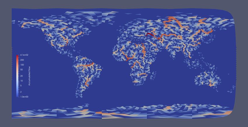
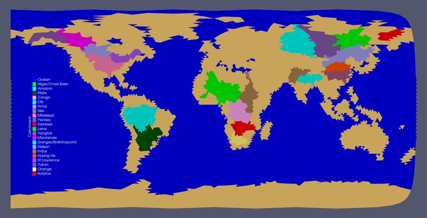
163 Results
The low resolution method without internal sinks was used to generate a set of river direction
for ICON r2b4 grid with the identifier (numberOfGridUsed) ‘0013’ [2] and the fractional-land
sea mask with identifier ‘0031’ as used by the Ruby-0 experiment of ICON-ESM. The minimum
fraction for a cell to be counted as land was taken as 50% (see section 2.6 for an explanation).
The catchments of major rivers for this setup are shown in Fig. 5 and the accumulated flows are
shown in Fig. 6.
17Figure 5: Major river catchments for an r2b4 grid setup.
18Figure 6: Accumulated flow (the number of cells upstream of a given grid cell) on a logarithmic
scale for an r2b4 grid setup.
1920
A     Instructions
A.1     General Notes
All the necessary tools are contained within the DynamicHD git repository and the parameter gen
eration scripts git submodule nested within it. Most of the tools are written in either C++ or
Fortran 2003. The interface for these tools differs between data on ICON icosahedral grids and
data on normal latitude-longitude grids. Tools for ICON icosahedral grids and cross-grid tools
are called from the command line specifying the settings, inputs and outputs via command line
arguments. Tools for latitude-longitude grids are called from Python using f2py and Cython to
call Fortran tools and C++ tools respectively. However, the tools required for creating ICON
hdpara files are run automatically by bash shell scripts. Thus, it should not be necessary to call
these tools directly. These tools all currently run on the Max Planck Institute for Meteorology
desktop linux system. Although in principle all these tools will work on Mistral, the correct
library paths and compiler options have not been set for this.

A.2     Instructions for Checking Out the Code
Instructions are provided for the bash shell on the Linux desktop system. These first steps are
common to all resolutions.

  1. Choose an appropriate base directory (${base directory path}) for the scripting.
            1   mkdir ${base directory path}

  2. Download the DynamicHD git repository from github and checkout the required tagged
     version:
            1   git clone https://github.com/ThomasRiddick/DynamicHD ${base directory path
                      ,→ }/DynamicHD
            2   cd ${base directory path}/DynamicHD
            3   git checkout icon hd tools version 1.2

  3. Install the parameter generation scripts git submodule into the DynamicHD repository
     (copying it from the contrib folder of the mpiesm−landveg repository):
            1   cd ${base directory path}/DynamicHD/Dynamic HD bash scripts
            2   rm −rf parameter generation scripts
            3   cd ${base directory path}
            4   git clone git.mpimet.mpg.de:mpiesm mpiesm−landveg
            5   cd mpiesm−landveg
            6   git checkout mpiesm−landveg
            7   git checkout 4e8167a679b5b85d7ae7710c14ecdb62fe4a024d
            8   cp −r contrib/dynamic hd code/Dynamic HD bash scripts/\
                      ,→ parameter generation scripts ${base directory path}/DynamicHD/\
                      ,→ Dynamic HD bash scripts

A.3     Instructions for Low Resolutions Without Internal Sinks
Instructions are provided for the bash shell on the Linux desktop system. If not using the ‘max
land’ option (counting all cells with any land as land) this procedure should be modified as detailed

                                                   21
in appendix A.7. Instructions for removing unfeasibly long retention times are given in appendix
A.6. A number of preliminary steps are not included in this description instead a set of files
produced by these preliminary steps that are valid for all possible setups is provided.
1. Check out the code according the instructions in appendix A.2.
2. Load the necessary models. First unload any existing modules. Then load anaconda3, cdo,
nco, and gcc/6.3.0
1 module load anaconda3
2 module load cdo
3 module load nco
4 module load gcc/6.3.0
3. Create a working directory for the ICON HD parameter generation process and change to
that directory:
1 cd ${base directory path}
2 mkdir hdpara gen workdir
4. Copy the necessary fixed input data from the linux system (login1) and the DynamicHD
git repository into this working directory:
1 cd hdpara gen workdir
2 cp ${base directory path}/DynamicHD/Dynamic HD Resources/\
,→ icon rdir gen top level config.cfg $(pwd)
3 cp ${base directory path}/DynamicHD/Dynamic HD Resources/\
,→ icon hdpara generation driver.cfg $(pwd)
4 scp username@mistral.dkrz.de:/pool/data/JSBACH/icon/HD\
,→ corrected orog intermediary ICE5G and tarasov upscaled srtm30plus\
,→ north america only data ALG4 sinkless glcc olson lsmask 0k 20170517\
,→ 003802 with grid.nc $(pwd)
5 scp username@mistral.dkrz.de:/pool/data/JSBACH/icon/HD\
,→ rdirs hydrosheds au af sa upscaled 10min 20200203 163646 corrg.nc $(\
,→ pwd)
5. Prepare a python environment for the scripts run (this will take some minutes to run):
1 ${base directory path}/DynamicHD/Dynamic HD bash scripts/\
,→ regenerate conda environment.sh
2 source activate dyhdenv
6. Edit the files icon rdir gen top level config.cfg and icon hdpara generation driver.cfg such that all
paths are correct for your system (and all field names match those used in the input files):
1 vim icon rdir gen top level config.cfg
2 vim icon hdpara generation driver.cfg
7. Run the main script6 :
6 It is possible at one stage during the script a loop (or several loops even) will be found that cannot be removed
automatically. If this is the case the script will prompt you to edit a river directions file on a 10 minute lat-lon
grid by hand to remove the loop. The loop can be identified with the loops log file and the catchment file. The
river directions file specified should be edited by hand using the nco command ncap2 to remove the loop(s) and
direct the water to the sea (the loop will usually be very close to the coast). Then enter the path of the edited
version of the file into the script as prompted and let it continue.
221 ${base directory path}/DynamicHD/Dynamic HD bash scripts/\
,→ generate icon hdpara top level driver.sh input icon orography.nc\
,→ input icon maximum land mask.nc output icon hdpara.nc\
,→ output icon catchments.nc output icon cumulative flow file.nc\
,→ icon rdir gen top level config.cfg $(pwd) input icon gridfile.nc ${\
,→ base directory path}/DynamicHD/Dynamic HD Resources/\
,→ cotat plus standard params.nl true
The script will produce a number of files. The key output file is the ICON hdpara file output icon hd
para.nc for input into the ICON model. Also important are the catchments for the generated river
directions on the ICON grid in output icon catchments.nc and the cumulative flows for the gen-
erated river directions on the ICON grid in output icon cumulative flow file.nc. The command line
arguments are as follows:
input orography filepath Input file containing an orography on the ICON grid. This is only
used to generate flow parameters and not for river directions.
input ls mask filepath Input file containing a binary land-sea mask on the ICON grid. In
this mask land points should have the value 1 and sea points should have the value 0.
output hdpara filepath Target filepath for the final ICON hdpara file produced by this script.
The file contains a number of fields, not all of which are currently used by JSBACH4. The
fields that are actually used by JSBACH4 are as follows:
MASK The HD model mask. -1 is denotes an ocean cell, 0 an ocean inflow cell, 1 a
normal land cell and 2 an internal drainage cell.
ALF K Overland flow retention coefficients. Units of days.
ALF N Number of overland flow reservoirs per cell. Currently always one for cells where
the HD model is run.
ARF K River flow retention coefficients. Units of days.
ARF N Number of river flow reservoirs per cell. Usually five for cells where the HD model
is run.
AGF K Base flow retention coefficients. Units of days.
CELLS UP Indices of neighbouring cells that flow directly into a given cell; act as a form
of river directions.
There is also an FDIR field which gives the index of the next cell directly downstream of
each cell, i.e. the river direction for that cell. This is not used directly but the information
in it is contained within the CELLS UP field which is derived from it.
output catchments filepath Target filepath for the final catchments (on the ICON grid) of
the ICON river directions created.
output accumulated flow filepath Target filepath for the final cumulative flow (on the ICON
grid) of the ICON river directions created.
config filepath A file specifying options for the top level bash script.
working directory Working directory to run this script in and place temporary files in. Mul-
tiple copies of this script cannot be run in the same working directory simultaneously.
23grid file The grid file describing the ICON grid to create an hdpara file for.
cotat params file Upscaling parameters for the upscaling algorithm. An appropriate file is
provided: DynamicHD/Dynamic HD Resources/cotat plus standard params.nl
compilation required Flag for compilation. Needs to be set to true the first time you run but
you can later set it to false to make the script run quicker
true sinks filepath (optional) A file containing the position of false sinks to use on a 10min
lat-lon grid. Not required when removing all internal basins.
Once an ICON hdpara file has been created, a check should be made that the final mask
matches the original input mask. This can be done using:
1 cdo expr,’lsm=(MASK==1 || MASK==2)’ output icon hdpara.nc mask from para.nc
2 cdo diff mask from para.nc input ls mask filepath.nc
This should result in zero differences. Occasionally there will be a difference in one or two
coastal cells. In this case the hdpara file should be edited by hand using the nco command ncap2
to remove any such differences.
The main routines of the script can be examined in:
DynamicHD/Dynamic HD bash scripts/generate icon hdpara top level driver.sh
and
DynamicHD/Dynamic HD Scripts/Dynamic HD Scripts/create icon coarse river directions driver.py
A.4 Instructions for Low Resolutions With Internal Sinks
Apart from a number of alterations detailed below, the same instructions should be followed as
for low resolutions without internal sinks. The alterations required are as follows:
• Endorheic/internal basins for Europe, Asia and North America can be added by providing a
true sinks file with the desired sink points flagged. The true sinks file should contain a field
of integers on a 10min latitude-longitude grid and its file path, true sinks filepath, should be
set as a final additional optional argument to generate icon hdpara top level driver.sh (as spec-
ified in the previous section). This file should be created by the user; no particular name
or location is required. One suggestion might be ${base directory path}/hdpara gen workdir
/true sinks.nc. To add internal basin find the lowest point in the basin in the 10min
latitude-longitude orography corrected orog intermediary ICE5G and tarasov upscaled srtm30plus
north america only data ALG4 sinkless glcc olson lsmask 0k 20170517 003802 with grid.nc. Insert
a true (value 1) flag at the corresponding point in the true sinks file. All other points in
this file are set to false (value 0).
• The Hydrosheds river directions include internal basins; some or all of these can be retained
when generating ICON river directions with internal sinks. Those that aren’t retained are
replaced as described in section 2.3. If you want to retain all the internal basins from
the Hydrosheds river directions the variable keep all internal basins should be set to True;
otherwise this variable should be set to False. If only some internal basin are to be re-
tained then which internal basins are retained can be set in icon hdpara generation driver.cfg
using either the variable replace only catchments or the variable exclude catchments. If set,
replace only catchments defines the selection of catchments that are replaced while all other
catchments are retained. Whereas if exclude catchments is set, it defines the selection of
internal basins that are retained and while all other catchments are replaced. Only one
24of these two variables should be specified in any given configuration. In either case, the
variable should be set to a list of catchment numbers separated by commas. The appropri-
ate catchment numbers for the individual Hydrosheds internal basins should be identified
using the ten minute catchments temp.nc file produced by a preliminary run of the script with
keep all internal basins set to True.
• How endorheic catchments that are removed are replaced depends on which variant is
being used (see section 2.3 for a description of the differences). Variant A (where water is
redirected towards the sea) is selected by setting replace internal basins with rdirs with tru
esinks=False. Variant B is selected by setting replace internal basins with rdirs with truesinks=
True. In variant B desired true sink points should also be specified in Africa, Australia
and South America (using the same true sinks file as for other regions). These can be
meaningfully specified even when within an internal catchment for which the Hydrosheds
river directions are being used (i.e. an internal catchment that has been ‘retained’). This
is the case because flagged true sinks can still be used to reconnect other minor endorheic
catchments with the given internal catchment in a logical way (i.e. across the lowest
point on the rims of basins) although the Hydrosheds river directions are used for the sink
containing catchment itself.
A.5 Instructions for High Resolutions Without Internal Sinks
Instructions are provided for the bash shell on the Linux desktop system. Instructions for remov-
ing unfeasibly long retention times are given in appendix A.6.
1. Check out the code according the instructions in appendix A.2.
2. Load the necessary models. First unload any existing modules. Then load cdo, nco, and
gcc/6.3.0:
1 module load cdo
2 module load nco
3 module load gcc/6.3.0
3. Prepare the environment and compile the C++ tools required:
1 export LD LIBRARY PATH=”/sw/stretch−x64/netcdf/netcdf fortran−4.4.4−
,→ gcc63/lib:/sw/stretch−x64/netcdf/netcdf c−4.6.1/lib:/sw/stretch−x64/
,→ netcdf/netcdf cxx−4.3.0−gccsys/lib:${LD LIBRARY PATH}”
2 cd ${base directory path}/DynamicHD
3 mkdir −p Dynamic HD Cpp Code/Release
4 mkdir −p Dynamic HD Cpp Code/Release/src
5 mkdir −p Dynamic HD Cpp Code/Release/src/base
6 mkdir −p Dynamic HD Cpp Code/Release/src/base/algorithms
7 mkdir −p Dynamic HD Cpp Code/Release/src/base/drivers
8 mkdir −p Dynamic HD Cpp Code/Release/src/base/testing
9 mkdir −p Dynamic HD Cpp Code/Release/src/base/command line drivers
10 cd Dynamic HD Cpp Code/Release
11 make −f ../makefile clean
12 make −f ../makefile tools only
4. Create a working directory for the ICON HD parameter generation process and change to
that directory:
251 cd ${base directory path}
2 mkdir hdpara gen workdir
5. Copy an orography, grid file and land-sea mask for the desired resolution to the working
directory:
1 cp /path/to/orography r2bX.nc ${base directory path}/hdpara gen workdir/\
,→ orography r2bX.nc
2 cp /path/to/landsea mask r2bX.nc ${base directory path}/hdpara gen workdir/\
,→ landsea mask r2bX.nc
3 cp gridfile r2bX.nc ${base directory path}/hdpara gen workdir/gridfile r2bX.nc
6. Edit paths in the script generate fine icon rdirs:
1 vim ${base directory path}/DynamicHD/Dynamic HD bash scripts/\
,→ generate fine icon rdirs
Set (replacing r2bX with the desired resolution):
1 icon data dir=${base directory path}/hdpara gen workdir/
2 cpp icon tool dir=${base directory path}/DynamicHD/Dynamic HD Cpp Code/\
,→ Release
3 grid file=${icon data dir}/gridfile r2bX.nc
4 orography file=${icon data dir}/orography r2bX.nc
5 lsmask file=${icon data dir}/landsea mask r2bX.nc
6 true sinks file=${icon data dir}/true sinks r2bX.nc
7 output orography file=${icon data dir}/orography r2bX filled.nc
8 next cell index file=${icon data dir}/rdirs r2bX.nc
9 catchments file=${icon data dir}/catchments r2bX.nc
7. Edit other settings in the script generate fine icon rdirs. Set the field names of required fields
in the input files:
1 input orography fieldname=”z”
2 input lsmask fieldname=”cell sea land mask”
3 input true sinks fieldname=”true sinks”
(Replacing ”z”, ”cell sea land mask” and ”true sinks” as appropriate.) Also set the flag for
fractional land-sea mask usage to the false value (which is in this case 0):
1 fractional lsmask flag=0
8. Run the river direction generation script:
1 cd ${base directory path}/hdpara gen workdir/
2 ${base directory path}/DynamicHD/Dynamic HD bash scripts/\
,→ generate fine icon rdirs
9. Run the parameter generation script7 :
7 Occasionally this code crashes because of a stray logging procedure. If this occurs change the value of ILOG to
1 in $base directory path/DynamicHD/DynamicHD/Dynamic HD bash scripts/parameter generation scripts
/fortran/paragen icon.f90, delete the intermediary files created by the first attempt and run again.
261 ${base directory path}/DynamicHD/Dynamic HD bash scripts/\
,→ parameter generation scripts/generate icon hd file driver.sh ${\
,→ base directory path}/hdpara gen workdir/ ${base directory path}/\
,→ DynamicHD/Dynamic HD bash scripts/parameter generation scripts/\
,→ fortran ${base directory path}/hdpara gen workdir/ ${\
,→ base directory path}/hdpara gen workdir/gridfile r2bX.nc ${\
,→ base directory path}/hdpara gen workdir/landsea mask r2bX.nc ${\
,→ base directory path}/hdpara gen workdir/rdirs r2bX.nc ${\
,→ base directory path}/hdpara gen workdir/orography r2bX filled.nc
The command line arguments are as follows:
workdir Working directory to use for running the script.
fortran src dir Directory containing the Fortran code for parameter generations; this is
usually a subdirectory of DynamicHD/Dynamic HD bash scripts/parameter generation scripts
named fortran.
base data dir Prefix to add to paths to input and output files.
grid file Input file containing ICON grid parameters.
lsmasks file Input file containing binary land-sea mask.
rdirs file Intermediary file produced by the previous step containing river directions in
the form of indices to the next cell downstream.
orography file Intermediary file produced by the previous step containing the filled orog-
raphy.
The final hdpara file (hdpara icon.nc) will be produced by this step.
10. The initial reservoirs values (hdstart.nc file) can be generated using the script create icon hdstart
included in JSBACH4 in scripts/preprocessing. The initial reservoirs will be interpolated from
a given MPI-ESM hdpara.nc. The follow variables need to set at the top of the script:
latlon initial file This should be a hdstart.nc file for MPI-ESM (JSBACH3) for the rele-
vant starting data from which the JSBACH4 file can be interpolated.
grid file The grid file for the relevant ICON grid.
landsea file The land-sea mask file for the relevant ICON grid.
landsea field The name of the land-sea mask field in the land-sea mask file.
label The label to attach to the output hdstart.nc file.
The output file produced by this will be named hdrestart [label].nc
A.6 Instructions for Adjusting Retention Coefficients
Instructions are provided for the bash shell on the Linux desktop system. These instructions follow
on from any of the other sets of instructions outlined above. It is assumed that the required code
has already been checked out according to the instructions in appendix A.2.
1. Plot a histogram of k-values for each flow type (out of river and overland flow) in visuali-
sation software such as paraview for the hdpara file that requires adjustment. Ignoring the
large spike at zero, find the value of retention coefficient for which the broad peak reaches
its maximum. Choose a cut-off above the end of the broad peak but below any scattered
individual peaks at much higher retention coefficient values.
272. Edit the file adjust icon k parameters.sh in the Dynamic HD bash scripts folder of the DynamicHD
repository to include/adjust the values for the resolution in question.
1 vim ${base directory path}/DynamicHD/Dynamic HD bash scripts/\
,→ adjust icon k parameters.sh
3. Load the nco module.
1 module load nco
4. Run adjust icon k parameters.sh with three command line arguments specifying the input
hdpara file to be modified, the name of the intended modified output hdpara file and the
resolution in question.
1 ${base directory path}/DynamicHD/Dynamic HD bash scripts/\
,→ adjust icon k parameters.sh input hdpara file.nc output hdpara file.nc \
,→ r2bX
A.7 Instructions for Using Fraction Land-Sea Mask
Instructions are provided for the bash shell on the Linux desktop system.
1. A binary land-sea mask with land defined as being cells with greater than a chosen threshold
fraction of land should be created using cdo commands. This should be used as the binary
land-sea mask in the generation of a hdpara file using one of the procedures detailed above
(usually that for low resolutions).
2. A second ‘max land’ binary land-sea mask should be created using cdo commands where
land is defined as all cells with greater than 0% land.
3. Change to an appropriate working directory containing the hdpara file produced and the
two binary land-sea masks.
4. Run the script adjust icon hdpara for partial ls.sh from the Dynamic HD bash scripts folder of the
DynamicHD repository with the ‘max land’ binary mask, the other binary mask, the path
of the input hdpara file, the target path for an output hdpara and an average value for
the overland flow retention coefficients to use to create the final hdpara file. The average
value for the overland flow retention coefficients should be chosen by histogramming the
overland flow retention coefficient values in the prior hdpara file and choosing the mode of
the broad peak of those values.
1 average overland flow retention coefficient value=X
2 ${base directory path}/DynamicHD/Dynamic HD bash scripts/\
,→ adjust icon hdpara for partial ls.sh maxland binary landsea mask.nc \
,→ land greater than Y binary landsea mask.nc input hdpara.nc \
,→ output hdpara.nc ${average overland flow retention coefficient value}
5. Minor modifications to the HD model are required to run JSBACH4 using this adjusted
hdpara file. These are already present in the latest version of JSBACH4.
28References
[1] Richard Barnes, Clarence Lehman, and David Mulla. Priority-flood: An optimal depression-
filling and watershed-labeling algorithm for digital elevation models. Comput. Geosci.,
62:117–127, 2014.
[2] Max Planck Institute for Meteorology. Icon grids: File register. http://icon-downloads.
mpimet.mpg.de/mpim_grids.xml. Last accessed 5th August 2021.
[3] S. Hagemann and L. Dümenil. Documentation for the hydrological discharge model. Tech-
nical Report 17, Max Planck Institute for Meteorology, Bundesstraße 55, 20146, Hamburg,
Germany, 1998.
[4] S. Hagemann and L. Dümenil. A parametrization of the lateral waterflow for the global
scale. Clim. Dynam., 14(1):17–31, 1998.
[5] Stefan Hagemann and Lydia Dümenil Gates. Validation of the hydrological cycle of ecmwf
and ncep reanalyses using the mpi hydrological discharge model. J. Geophys. Res.-Atmos.,
106(D2):1503–1510, 2001.
[6] M. Latif, M. Claussen, M. Schulz, and T. Brücher. Comprehensive earth system models of
the last glacial cycle. EOS, 97, 2016.
[7] Bernhard Lehner, Kristine Verdin, and Andy Jarvis. New global hydrography derived from
spaceborne elevation data. EOS, 89(10):93–94, 2008.
[8] Adriano Rolim Paz, Walter Collischonn, and André Luiz Lopes da Silveira. Improvements
in large-scale drainage networks derived from digital elevation models. Water Resour. Res.,
42, W08502, 2006.
[9] W.R. Peltier. Global glacial isostasy and the surface of the ice-age earth: the ice-5g (vm2)
model and grace. Annu. Rev. Earth Pl. Sc., 32:111–149, 2004.
[10] T. Riddick, V. Brovkin, S. Hagemann, and U. Mikolajewicz. Dynamic hydrological discharge
modelling for coupled climate model simulations of the last glacial cycle: the mpi-dynamichd
model version 3.0. Geosci. Model Dev., 11(10):4291–4316, 2018.
[11] D. Yamazaki, T. Oki, and S. Kanae. Deriving a global river network map and its sub-grid
topographic characteristics from a fine-resolution flow direction map. Hydrol. Earth Syst.
Sc., 13(11):2241–2251, 2009.
[12] Dai Yamazaki, Daiki Ikeshima, Jeison Sosa, Paul D. Bates, George H. Allen, and Tam-
lin M. Pavelsky. Merit hydro: A high-resolution global hydrography map based on latest
topography dataset. Water Resour. Res., 55(6):5053–5073, 2019.
29You can also read