TRUSTNLP: FIRST WORKSHOP ON TRUSTWORTHY NATURAL LANGUAGE PROCESSING PROCEEDINGS OF THE WORKSHOP - TRUSTNLP - JUNE 10, 2021
←
→
Page content transcription
If your browser does not render page correctly, please read the page content below
TrustNLP

TrustNLP: First Workshop on Trustworthy Natural
              Language Processing

          Proceedings of the Workshop

                 June 10, 2021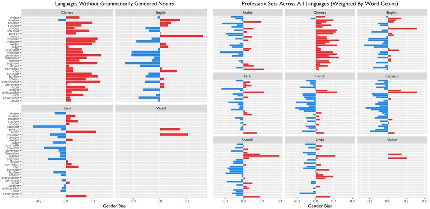
©2021 The Association for Computational Linguistics

Order copies of this and other ACL proceedings from:

             Association for Computational Linguistics (ACL)
             209 N. Eighth Street
             Stroudsburg, PA 18360
             USA
             Tel: +1-570-476-8006
             Fax: +1-570-476-0860
             acl@aclweb.org

ISBN 978-1-954085-33-6

                                            ii
Introduction

Recent progress in Artificial Intelligence (AI) and Natural Language Processing (NLP) has greatly
increased their presence in everyday consumer products in the last decade. Common examples
include virtual assistants, recommendation systems, and personal healthcare management systems,
among others. Advancements in these fields have historically been driven by the goal of improving
model performance as measured by accuracy, but recently the NLP research community has started
incorporating additional constraints to make sure models are fair and privacy-preserving. However, these
constraints are not often considered together, which is important since there are critical questions at the
intersection of these constraints such as the tension between simultaneously meeting privacy objectives
and fairness objectives, which requires knowledge about the demographics a user belongs to. In this
workshop, we aim to bring together these distinct yet closely related topics.

We invited papers which focus on developing models that are “explainable, fair, privacy-preserving,
causal, and robust” (Trustworthy ML Initiative). Topics of interest include:

    • Differential Privacy

    • Fairness and Bias: Evaluation and Treatments

    • Model Explainability and Interpretability

    • Accountability

    • Ethics

    • Industry applications of Trustworthy NLP

    • Causal Inference

    • Secure and trustworthy data generation

In total, we accepted 11 papers, including 2 non-archival papers. We hope all the attendants enjoy this
workshop.

                                                    iii
Organizing Committee
• Yada Pruksachatkun - Alexa AI
• Anil Ramakrishna - Alexa AI
• Kai-Wei Chang - UCLA, Amazon Visiting Academic
• Satyapriya Krishna - Alexa AI
• Jwala Dhamala - Alexa AI
• Tanaya Guha - University of Warwick
• Xiang Ren - USC
Speakers
• Mandy Korpusik - Assistant professor, Loyola Marymount University
• Richard Zemel - Industrial Research Chair in Machine Learning, University of Toronto
• Robert Monarch - Author, Human-in-the-Loop Machine Learning
Program committee
• Rahul Gupta - Alexa AI
• Willie Boag - Massachusetts Institute of Technology
• Naveen Kumar - Disney Research
• Nikita Nangia - New York University
• He He - New York University
• Jieyu Zhao - University of California Los Angeles
• Nanyun Peng - University of California Los Angeles
• Spandana Gella - Alexa AI
• Moin Nadeem - Massachusetts Institute of Technology
• Maarten Sap - University of Washington
• Tianlu Wang - University of Virginia
• William Wang - University of Santa Barbara
• Joe Near - University of Vermont
• David Darais - Galois
• Pratik Gajane - Department of Computer Science, Montanuniversitat Leoben, Austria
• Paul Pu Liang - Carnegie Mellon University
v• Hila Gonen - Bar-Ilan University
• Patricia Thaine - University of Toronto
• Jamie Hayes - Google DeepMind, University College London, UK
• Emily Sheng - University of California Los Angeles
• Isar Nejadgholi - National Research Council Canada
• Anthony Rios - University of Texas at San Antonio
viTable of Contents
Interpretability Rules: Jointly Bootstrapping a Neural Relation Extractorwith an Explanation Decoder
Zheng Tang and Mihai Surdeanu . . . . . . . . . . . . . . . . . . . . . . . . . . . . . . . . . . . . . . . . . . . . . . . . . . . . . . . . . . 1
Measuring Biases of Word Embeddings: What Similarity Measures and Descriptive Statistics to Use?
Hossein Azarpanah and Mohsen Farhadloo . . . . . . . . . . . . . . . . . . . . . . . . . . . . . . . . . . . . . . . . . . . . . . . . . 8
Private Release of Text Embedding Vectors
Oluwaseyi Feyisetan and Shiva Kasiviswanathan . . . . . . . . . . . . . . . . . . . . . . . . . . . . . . . . . . . . . . . . . . . 15
Accountable Error Characterization
Amita Misra, Zhe Liu and Jalal Mahmud . . . . . . . . . . . . . . . . . . . . . . . . . . . . . . . . . . . . . . . . . . . . . . . . . . 28
xER: An Explainable Model for Entity Resolution using an Efficient Solution for the Clique Partitioning
Problem
Samhita Vadrevu, Rakesh Nagi, JinJun Xiong and Wen-mei Hwu . . . . . . . . . . . . . . . . . . . . . . . . . . . . 34
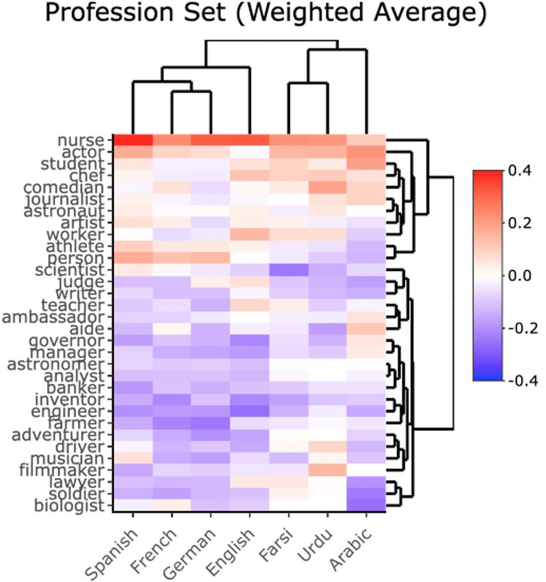
Gender Bias in Natural Language Processing Across Human Languages
Abigail Matthews, Isabella Grasso, Christopher Mahoney, Yan Chen, Esma Wali, Thomas Middle-
ton, Mariama Njie and Jeanna Matthews . . . . . . . . . . . . . . . . . . . . . . . . . . . . . . . . . . . . . . . . . . . . . . . . . . . . . . . 45
Interpreting Text Classifiers by Learning Context-sensitive Influence of Words
Sawan Kumar, Kalpit Dixit and Kashif Shah . . . . . . . . . . . . . . . . . . . . . . . . . . . . . . . . . . . . . . . . . . . . . . . 55
Towards Benchmarking the Utility of Explanations for Model Debugging
Maximilian Idahl, Lijun Lyu, Ujwal Gadiraju and Avishek Anand . . . . . . . . . . . . . . . . . . . . . . . . . . . 68
viiConference Program
June 10, 2021
9:00–9:10 Opening
Organizers
9:10–10:00 Keynote 1
Richard Zemel
10:00–11:00 Paper Presentations
Interpretability Rules: Jointly Bootstrapping a Neural Relation Extractorwith an
Explanation Decoder
Zheng Tang and Mihai Surdeanu
Measuring Biases of Word Embeddings: What Similarity Measures and Descriptive
Statistics to Use?
Hossein Azarpanah and Mohsen Farhadloo
Private Release of Text Embedding Vectors
Oluwaseyi Feyisetan and Shiva Kasiviswanathan
Accountable Error Characterization
Amita Misra, Zhe Liu and Jalal Mahmud
11:00–11:15 Break
ixJune 10, 2021 (continued)
11:15–12:15 Paper Presentations
xER: An Explainable Model for Entity Resolution using an Efficient Solution for the
Clique Partitioning Problem
Samhita Vadrevu, Rakesh Nagi, JinJun Xiong and Wen-mei Hwu
Gender Bias in Natural Language Processing Across Human Languages
Abigail Matthews, Isabella Grasso, Christopher Mahoney, Yan Chen, Esma Wali,
Thomas Middleton, Mariama Njie and Jeanna Matthews
Interpreting Text Classifiers by Learning Context-sensitive Influence of Words
Sawan Kumar, Kalpit Dixit and Kashif Shah
Towards Benchmarking the Utility of Explanations for Model Debugging
Maximilian Idahl, Lijun Lyu, Ujwal Gadiraju and Avishek Anand
12:15–1:30 Lunch Break
13:00–14:00 Mentorship Meeting
14:00–14:50 Keynote 2
Mandy Korpusik
14:50–15:00 Break
15:00–16:00 Poster Session
16:15–17:05 Keynote 3
Robert Munro
17:05–17:15 Closing Address
xInterpretability Rules: Jointly Bootstrapping a Neural Relation Extractor
with an Explanation Decoder
Zheng Tang, Mihai Surdeanu
Department of Computer Science
University of Arizona, Tucson, Arizona, USA
{zhengtang, msurdeanu}@email.arizona.edu
Abstract traction (RE) system (Angeli et al., 2015) and boot-
strap a neural RE approach that is trained jointly
We introduce a method that transforms a rule-
with a decoder that learns to generate the rules that
based relation extraction (RE) classifier into
a neural one such that both interpretability
best explain each particular extraction. The contri-
and performance are achieved. Our approach butions of our idea are the following:
jointly trains a RE classifier with a decoder (1) We introduce a strategy that jointly learns a RE
that generates explanations for these extrac- classifier between pairs of entity mentions with a
tions, using as sole supervision a set of rules
decoder that generates explanations for these ex-
that match these relations. Our evaluation on
the TACRED dataset shows that our neural RE tractions in the form of Tokensregex (Chang and
classifier outperforms the rule-based one we Manning, 2014) or Semregex (Chambers et al.,
started from by 9 F1 points; our decoder gen- 2007) patterns. The only supervision for our
erates explanations with a high BLEU score of method is a set of input rules (or patterns) in these
over 90%; and, the joint learning improves the two frameworks (Angeli et al., 2015), which we
performance of both the classifier and decoder. use to generate positive examples for both the clas-
sifier and the decoder. We generate negative exam-
1 Introduction
ples automatically from the sentences that contain
Information extraction (IE) is one of the key chal- positives examples.
lenges in the natural language processing (NLP) (2) We evaluate our approach on the TACRED
field. With the explosion of unstructured informa- dataset (Zhang et al., 2017) and demonstrate that:
tion on the Internet, the demand for high-quality (a) our neural RE classifier outperforms consider-
tools that convert free text to structured information ably the rule-based one we started from; (b) our
continues to grow (Chang et al., 2010; Lee et al., decoder generates explanations with high accuracy,
2013; Valenzuela-Escarcega et al., 2018). i.e., a BLEU overlap score between the generated
The past decades have seen a steady transition rules and the gold, hand-written rules of over 90%;
from rule-based IE systems (Appelt et al., 1993) to and, (c) joint learning improves the performance of
methods that rely on machine learning (ML) (see both the classifier and decoder.
Related Work). While this transition has generally
yielded considerable performance improvements, it (3) We demonstrate that our approach generalizes
was not without a cost. For example, in contrast to to the situation where a vast amount of labeled
modern deep learning methods, the predictions of training data is combined with a few rules. We com-
rule-based approaches are easily explainable, as a bined the TACRED training data with the above
small number of rules tends to apply to each extrac- rules and showed that when our method is trained
tion. Further, in many situations, rule-based meth- on this combined data, the classifier obtains near
ods can be developed by domain experts with mini- state-of-art performance at 67.0% F1, while the de-
mal training data. For these reasons, rule-based IE coder generates accurate explanations with a BLEU
methods remain widely used in industry (Chiticariu score of 92.4%.
et al., 2013).
2 Related Work
In this work we demonstrate that this transition
from rule- to ML-based IE can be performed such Relation extraction using statistical methods is
that the benefits of both worlds are preserved. In well studied. Methods range from supervised,
particular, we start with a rule-based relation ex- “traditional” approaches (Zelenko et al., 2003;
1
Proceedings of the First Workshop on Trustworthy Natural Language Processing, pages 1–7
June 10, 2021. ©2021 Association for Computational LinguisticsBunescu and Mooney, 2005) to neural meth- 3.1 Task 1: Relation Classifier
ods. Neural approaches for RE range from meth- We define the RE task as follows. The inputs con-
ods that rely on simpler representations such as sist of a sentence W = [w1 , . . . , wn ], and a pair
CNNs (Zeng et al., 2014) and RNNs (Zhang and of entities (called “subject” and “object”) corre-
Wang, 2015) to more complicated ones such as sponding to two spans in this sentence: Ws =
augmenting RNNs with different components (Xu [ws1 , . . . , wsn ] and Wo = [wo1 , . . . , won ]. The
et al., 2015; Zhou et al., 2016), combining RNNs goal is to predict a relation r ∈ R (from a pre-
and CNNs (Vu et al., 2016; Wang et al., 2016), defined set of relation types) that holds between the
and using mechanisms like attention (Zhang et al., subject and object or “no relation” otherwise.
2017) or GCNs (Zhang et al., 2018). To solve the For each sentence, we associate each word wi
lack of annotated data, distant supervision (Mintz with a representation x i that concatenates three
et al., 2009; Surdeanu et al., 2012) is commonly embeddings: x i = e (wi ) ◦ e (ni ) ◦ e (pi ), where
used to generate a training dataset from an existing e (wi ) is the word embedding of token i, e (ni ) is
knowledge base. Jat et al. (2018) address the in- the NER embedding of token i, e (pi ) is the POS
herent noise in distant supervision with an entity Tag embedding of token i. We feed these represen-
attention method. tations into a sentence-level bidirectional LSTM
Rule-based methods in IE have also been ex- encoder (Hochreiter and Schmidhuber, 1997):
tensively investigated. Riloff (1996) developed a
system that learns extraction patterns using only h1 , . . . , h n ] = LSTM([x
[h x1 , . . . , x n ]) (1)
a pre-classified corpus of relevant and irrelevant
texts. Lin and Pantel (2001) proposed a unsuper- Following (Zhang et al., 2018), we extract the
vised method for discovering inference rules from “K-1 pruned” dependency tree that covers the two
text based on the Harris distributional similarity entities, i.e., the shortest dependency path between
hypothesis (Harris, 1954). Valenzuela-Escárcega two entities enhanced with all tokens that are di-
et al. (2016) introduced a rule language that covers rectly attached to the path, and feed it into a
both surface text and syntactic dependency graphs. GCN (Kipf and Welling, 2016) layer:
Angeli et al. (2015) further show that converting Xn
rule-based models to statistical ones can capture (l)
h i = σ(
(l−1)
Ãij W (l)h j /di + b (l) ) (2)
some of the benefits of both, i.e., the precision of j=1
patterns and the generalizability of statistical mod- where A is the corresponding adjacency matrix,
els. Ã = AP + I with I being the n × n identity matrix,
Interpretability has gained more attention re- n
di = j=1 Ãij is the degree of token i in the
cently in the ML/NLP community. For example,
resulting graph, and W (l) is linear transformation.
some efforts convert neural models to more inter-
Lastly, we concatenate the sentence represen-
pretable ones such as decision trees (Craven and
tation, the subject entity representation, and the
Shavlik, 1996; Frosst and Hinton, 2017). Some
object entity representation as follows:
others focus on producing a post-hoc explanation
of individual model outputs (Ribeiro et al., 2016; h(L) ) = f (GCN(h
h sent = f (h h(0 )) (3)
Hendricks et al., 2016).
h(L)
h s = f (h s1 :sn ) (4)
Inspired by these directions, here we propose
an approach that combines the interpretability of
h(L)
h o = f (h o1 :on ) (5)
rule-based methods with the performance and gen-
eralizability of neural approaches. h f inal = h sent ◦ h s ◦ h o (6)
3 Approach
where h (l) denotes the collective hidden repre-
Our approach jointly addresses classification and sentations at layer l of the GCN, and f : Rd×n →
interpretability through an encoder-decoder archi- Rd is a max pooling function that maps from n
tecture, where the decoder uses multi-task learn- output vectors to the representation vector. The
ing (MTL) for relation extraction between pairs of concatenated representation h f inal is fed to a feed-
named entities (Task 1) and rule generation (Task forward layer with a softmax function to produce a
2). Figure 1 summarizes our approach. probability distribution over relation types.
2Figure 1: Neural architecture of the proposed multitask learning approach. The input is a sequence of words
together with NER labels and POS tags. The pair of entities to be classified (“subject” in blue and “object” in
orange) are also provided. We use a concatenation of several representations, including embeddings of words, NER
labels, and POS tags. The encoder uses a sentence-level bidirectional LSTM (biLSTM) and graph convolutional
networks (GCN). There are pooling layers for the subject, object, and full sentence GCN outputs. The concatenated
pooling outputs are fed to the classifier’s feedforward layer. The decoder is an LSTM with an attention mechanism.
3.2 Task 2: Rule Decoder Approach Precision Recall F1 BLEU
Rule-only data
The rule decoder’s goal is to generate the pat- Rule baseline 86.9 23.2 36.6 –
Our approach 60.0 36.7 45.5 90.3
tern P that extracted the corresponding data w/o decoder 58.7 36.4 44.9 –
point, where P is represented as a sequence w/o classifier – – – 88.3
of tokens in the corresponding pattern lan- Rules + TACRED training data
C-GCN 69.9 63.3 66.4 –
guage: P = [p1 , . . . , pn ]. For example, the Our approach 70.2 64.0 67.0 92.4
pattern (([{kbpentity:true}]+)/was/ w/o decoder 71.2 62.3 66.5 –
/born/ /on/([{slotvalue:true}]+)) w/o classifier – – – 91.6
(where kbpentity:true marks subject tokens,
Table 1: Results on the TACRED test partition, includ-
and slotvalue:true marks object tokens) ing ablation experiments (the “w/o” rows). We exper-
extracts mentions of the per:date_of_birth imented with two configurations: Rule-only data uses
relation. only training examples generated by rules; Rules + TA-
We implemented this decoder using an LSTM CRED training data applies the previous rules to the
with an attention mechanism. To center rule decod- training dataset from TACRED.
ing around the subject and object, we first feed the
concatenation of subject and object representation use its output to obtain a probability distribution
from the encoder as the initial state in the decoder. over the pattern vocabulary.
Then, in each timestep t, we generate the attention We use cross entropy to calculate the losses for
context vector C D
t by using the current hidden state both the classifier and decoder. To balance the loss
of the decoder, h D
t : between classifier and decoder, we normalize the
s t (j) = h E A D
(7) decoder loss by the pattern length. Note that for
(L)W h t
the data points without an existing rule, we only
calculate the classifier loss. Formally, the joint loss
a t = softmax(sst ) (8)
function is:
X
CD
t = hE
a t (j)h j (9) loss = lossc + lossd /length(P ) (10)
j
where W A is a learned matrix, and h E(L) are hid- 4 Experiments
den representations from the encoder’s GCN.
We feed this C D
t vector to a single feed forward Data Preparation: We report results on the TA-
layer that is coupled with a softmax function and CRED dataset (Zhang et al., 2017). We bootstrap
3Hand-written Rule Decoded Rule
(([{kbpentity:true}]+)""" based ""in"([{slotvalue:true}]+)) (([{kbpentity:true}]+)"in"([{slotvalue:true}]+))
(([{kbpentity:true}]+)" CEO "([{slotvalue:true}]+)) (([{kbpentity:true}]+)" president "([{slotvalue:true}]+))
Table 2: Examples of mistakes in the decoded rules. We highlight in the hand-written rules the tokens that were
missed during decoding (false negatives) in green, and in the decoded rules we highlight the spurious tokens (false
positives) in red.
Model Precision Recall F1 BLEU our word embeddings. We use the Adagrad opti-
20% of rules 74.9 20.1 31.7 96.9
40% of rules 69.0 26.9 38.8 90.8 mizer (Duchi et al., 2011). We apply entity mask-
60% of rules 62.7 29.7 40.3 88.8 ing to subject and object entities in the sentence,
80% of rules 57.3 36.5 44.6 89.4 which is replacing the original token with a spe-
Table 3: Learning curve of our approach based on cial –SUBJ or –OBJ token where
amount of rules used, in the rule-only data configura- is the corresponding name entity label pro-
tion. These results are on TACRED development. vided by TACRED.
We used micro precision, recall, and F1 scores
to evaluate the RE classifier. We used the BLEU
our models from the patterns in the rule-based sys-
score to measure the quality of generated rules, i.e.,
tem of Angeli et al. (2015), which uses 4,528 sur-
how close they are to the corresponding gold rules
face patterns (in the Tokensregex language) and
that extracted the same output. We used the BLEU
169 patterns over syntactic dependencies (using
implementation in NLTK (Loper and Bird, 2002),
Semgrex). We experimented with two configura-
which allows us to calculate multi-reference BLEU
tions: rule-only data and rules + TACRED training
scores over 1 to 4 grams.4 We report BLEU scores
data. In the former setting, we use solely pos-
only over the non ’no_relation’ extractions with the
itive training examples generated by the above
corresponding testing data points that are matched
rules. We combine these positive examples with
by one of the rules in (Zhang et al., 2017).
negative ones generated automatically by assigning
’no_relation’ to all other entity mention pairs in the Results and Discussion: Table 1 reports the
same sentence where there is a positive example.1 overall performance of our approach, the baselines,
We generated 3,850 positive and 12,311 negative and ablation settings, for the two configurations
examples for this configuration. In the latter con- investigated. We draw the following observations
figuration, we apply the same rules to the entire from these results:
TACRED training dataset.2
(1) The rule-based method of Zhang et al. (2017)
Baselines: We compare our approach with two has high precision but suffers from low recall. In
baselines: the rule-based system of Zhang et al. contrast, our approach that is bootstrapped from the
(2017), and the best non-combination method of same information has 13% higher recall and almost
Zhang et al. (2018). The latter method uses an 9% higher F1 (absolute). Further, our approach
LSTM and GCN combination similar to our en- decodes explanatory rules with a high BLEU score
coder.3 of 90%, which indicates that it maintains almost the
entire explanatory power of the rule-based method.
Implementation Details: We use pre-trained
(2) The ablation experiments indicate that joint
GloVe vectors (Pennington et al., 2014) to initialize
training for classification and explainability helps
1
During the generation of these negative examples we both tasks, in both configurations. This indi-
filtered out pairs corresponding to inverse and symmetric re-
lations. For example, if a sentence contains a relation (Subj,
cates that performance and explainability are inter-
Rel, Obj), we do not generate the negative (Obj, no_relation, connected.
Subj) if Rel has an inverse relation, e.g., per:children is
the inverse of per:parents. (3) The two configurations analyzed in the table
2
Thus, some training examples in this case will be asso- demonstrate that our approach performs well not
ciated with a rule and some will not. We adjusted the loss only when trained solely on rules, but also when
function to use only the classification loss when no rule ap-
plies. rules are combined with a training dataset anno-
3
For a fair comparison, we do not compare against ensem- tated for RE. This suggests that our direction may
ble methods, or transformer-based ones. Also, note that this
4
baseline does not use rules at all. We scored longer n-grams to better capture rule syntax.
4be a general strategy to infuse some explainability that provided the training patterns by 9 F1 points,
in a statistical method, when rules are available while decoding explanations at over 90% BLEU
during training. score. Further, we showed that the joint training
(4) Table 3 lists the learning curve for our ap- of the classification and explanation components
proach in the rule-only data configuration when performs better than training them separately. All
the amount of rules available varies.5 This table in all, our work suggests that it is possible to marry
shows that our approach obtains a higher F1 than the interpretability of rule-based methods with the
the complete rule-based RE classifier even when performance of neural approaches.
using only 40% of the rules.6
(5) Note that the BLEU score provides an incom- References
plete evaluation of rule quality. To understand if
Gabor Angeli, Victor Zhong, Danqi Chen, A. Cha-
the decoded rules explain their corresponding data ganty, J. Bolton, Melvin Jose Johnson Premkumar,
point, we performed a manual evaluation on 176 Panupong Pasupat, S. Gupta, and Christopher D.
decoded rules. We classified them into three cate- Manning. 2015. Bootstrapped self training for
gories: (a) the rules correctly explain the prediction knowledge base population. Theory and Applica-
tions of Categories.
(according to the human annotator), (b) they ap-
proximately explain the prediction, and (c) they Douglas E Appelt, Jerry R Hobbs, John Bear, David Is-
do not explain the prediction. Class (b) contains rael, and Mabry Tyson. 1993. Fastus: A finite-state
rules that do not lexically match the input text, processor for information extraction from real-world
text. In IJCAI, volume 93, pages 1172–1178.
but capture the correct semantics, as shown in Ta-
ble 2. The percentages we measured were: (a) Razvan Bunescu and Raymond Mooney. 2005. A
33.5%, (b) 31.3%, (c) 26.1%. 9% of these rules shortest path dependency kernel for relation extrac-
tion. In Proceedings of Human Language Technol-
were skipped in the evaluation because they were ogy Conference and Conference on Empirical Meth-
false negatives( which are labeled as no relation ods in Natural Language Processing, pages 724–
falsely by our model). These numbers support our 731.
hypothesis that, in general, the decoded rules do
Nathanael Chambers, Daniel Cer, Trond Grenager,
explain the classifier’s prediction. David Hall, Chloe Kiddon, Bill MacCartney, Marie-
Further, out of 750 data points associated with Catherine de Marneffe, Daniel Ramage, Eric Yeh,
rules in the evaluation data, our method incorrectly and Christopher D. Manning. 2007. Learning align-
classifies only 26. Out of these 26, 16 were false ments and leveraging natural logic. In Proceedings
of the ACL-PASCAL Workshop on Textual Entail-
negatives, and had no rules decoded. In the other 10 ment and Paraphrasing, pages 165–170, Prague. As-
predictions, 7 rules fell in class (b) (see the exam- sociation for Computational Linguistics.
ples in Table 2). The other 3 were incorrect due to
Angel X Chang and Christopher D Manning. 2014. To-
ambiguity, i.e., the pattern created is an ambiguous kensregex: Defining cascaded regular expressions
succession of POS tags or syntactic dependencies over tokens. Stanford University Computer Science
without any lexicalization. This suggests that, even Technical Reports. CSTR, 2:2014.
when our classifier is incorrect, the rules decoded
Angel X Chang, Valentin I Spitkovsky, Eric Yeh,
tend to capture the underlying semantics. Eneko Agirre, and Christopher D Manning. 2010.
Stanford-ubc entity linking at tac-kbp.
5 Conclusion
Laura Chiticariu, Yunyao Li, and Frederick Reiss. 2013.
We introduced a strategy that jointly bootstraps a Rule-based information extraction is dead! long live
relation extraction classifier with a decoder that rule-based information extraction systems! In Pro-
generates explanations for these extractions, us- ceedings of the 2013 conference on empirical meth-
ods in natural language processing, pages 827–832.
ing as sole supervision a set of example patterns
that match such relations. Our experiments on Mark Craven and Jude W Shavlik. 1996. Extracting
the TACRED dataset demonstrated that our ap- tree-structured representations of trained networks.
In Advances in neural information processing sys-
proach outperforms the strong rule-based method
tems, pages 24–30.
5
For this experiment we sorted the rules in descending
order of their match frequency in training, and kept the top John Duchi, Elad Hazan, and Yoram Singer. 2011.
n% in each setting. Adaptive subgradient methods for online learning
6
The high BLEU score in the 20% configuration is due to and stochastic optimization. Journal of machine
the small sample in development for which gold rules exist. learning research, 12(7).
5Nicholas Frosst and Geoffrey Hinton. 2017. Distilling Marco Tulio Ribeiro, Sameer Singh, and Carlos
a neural network into a soft decision tree. arXiv Guestrin. 2016. Why should i trust you?: Explain-
preprint arXiv:1711.09784. ing the predictions of any classifier. In Proceed-
ings of the 22nd ACM SIGKDD international con-
Zellig S Harris. 1954. Distributional structure. Word, ference on knowledge discovery and data mining,
10(2-3):146–162. pages 1135–1144. ACM.
Lisa Anne Hendricks, Zeynep Akata, Marcus Ellen Riloff. 1996. Automatically generating extrac-
Rohrbach, Jeff Donahue, Bernt Schiele, and Trevor tion patterns from untagged text. In Proceedings
Darrell. 2016. Generating visual explanations. In of the national conference on artificial intelligence,
European Conference on Computer Vision, pages pages 1044–1049.
3–19. Springer.
Mihai Surdeanu, Julie Tibshirani, Ramesh Nallapati,
and Christopher D. Manning. 2012. Multi-instance
Sepp Hochreiter and Jürgen Schmidhuber. 1997.
multi-label learning for relation extraction. In Pro-
Long short-term memory. Neural computation,
ceedings of the 2012 Joint Conference on Empirical
9(8):1735–1780.
Methods in Natural Language Processing and Com-
putational Natural Language Learning, pages 455–
Sharmistha Jat, Siddhesh Khandelwal, and Partha
465, Jeju Island, Korea. Association for Computa-
Talukdar. 2018. Improving distantly supervised rela-
tional Linguistics.
tion extraction using word and entity based attention.
arXiv preprint arXiv:1804.06987. Marco A. Valenzuela-Escarcega, Ozgun Babur, Gus
Hahn-Powell, Dane Bell, Thomas Hicks, Enrique
Thomas N Kipf and Max Welling. 2016. Semi- Noriega-Atala, Xia Wang, Mihai Surdeanu, Emek
supervised classification with graph convolutional Demir, and Clayton T. Morrison. 2018. Large-scale
networks. arXiv preprint arXiv:1609.02907. automated machine reading discovers new cancer
driving mechanisms. Database: The Journal of Bio-
Heeyoung Lee, Angel Chang, Yves Peirsman, logical Databases and Curation.
Nathanael Chambers, Mihai Surdeanu, and Dan
Jurafsky. 2013. Deterministic coreference reso- Marco A. Valenzuela-Escárcega, Gus Hahn-Powell,
lution based on entity-centric, precision-ranked and Mihai Surdeanu. 2016. Odin’s runes: A rule lan-
rules. Computational Linguistics, 39(4):885–916. guage for information extraction. In Proceedings of
Copyright: Copyright 2020 Elsevier B.V., All rights the Tenth International Conference on Language Re-
reserved. sources and Evaluation (LREC’16), pages 322–329,
Portorož, Slovenia. European Language Resources
Dekang Lin and P. Pantel. 2001. Dirt – discovery of Association (ELRA).
inference rules from text.
Ngoc Thang Vu, Heike Adel, Pankaj Gupta, and Hin-
Edward Loper and Steven Bird. 2002. Nltk: The natu- rich Schütze. 2016. Combining recurrent and con-
ral language toolkit. In In Proceedings of the ACL volutional neural networks for relation classification.
Workshop on Effective Tools and Methodologies for In Proceedings of the 2016 Conference of the North
Teaching Natural Language Processing and Compu- American Chapter of the Association for Computa-
tational Linguistics. Philadelphia: Association for tional Linguistics: Human Language Technologies,
Computational Linguistics. pages 534–539, San Diego, California. Association
for Computational Linguistics.
Christopher D. Manning, Mihai Surdeanu, John Bauer,
Linlin Wang, Zhu Cao, Gerard de Melo, and Zhiyuan
Jenny Finkel, Steven J. Bethard, and David Mc-
Liu. 2016. Relation classification via multi-level
Closky. 2014. The Stanford CoreNLP natural lan-
attention CNNs. In Proceedings of the 54th An-
guage processing toolkit. In Association for Compu-
nual Meeting of the Association for Computational
tational Linguistics (ACL) System Demonstrations,
Linguistics (Volume 1: Long Papers), pages 1298–
pages 55–60.
1307, Berlin, Germany. Association for Computa-
tional Linguistics.
Mike Mintz, Steven Bills, Rion Snow, and Dan Juraf-
sky. 2009. Distant supervision for relation extrac- Yan Xu, Lili Mou, Ge Li, Yunchuan Chen, Hao Peng,
tion without labeled data. In Proceedings of the and Zhi Jin. 2015. Classifying relations via long
Joint Conference of the 47th Annual Meeting of the short term memory networks along shortest depen-
ACL and the 4th International Joint Conference on dency paths. In Proceedings of the 2015 Conference
Natural Language Processing of the AFNLP, pages on Empirical Methods in Natural Language Process-
1003–1011. ing, pages 1785–1794, Lisbon, Portugal. Associa-
tion for Computational Linguistics.
Jeffrey Pennington, Richard Socher, and Christopher D
Manning. 2014. Glove: Global vectors for word rep- Dmitry Zelenko, Chinatsu Aone, and Anthony
resentation. In Proceedings of the 2014 conference Richardella. 2003. Kernel methods for relation ex-
on empirical methods in natural language process- traction. Journal of machine learning research,
ing (EMNLP), pages 1532–1543. 3(Feb):1083–1106.
6Daojian Zeng, Kang Liu, Siwei Lai, Guangyou Zhou, Encoder and classifier components Size
and Jun Zhao. 2014. Relation classification via con- Vocabulary 53953
volutional deep neural network. In Proceedings of POS embedding dimension 30
COLING 2014, the 25th International Conference
on Computational Linguistics: Technical Papers, NER embedding dimension 30
pages 2335–2344. LSTM hidden layers 200
Feedforward layers 200
Dongxu Zhang and Dong Wang. 2015. Relation classi- GCN layers 200
fication via recurrent neural network. arXiv preprint
arXiv:1508.01006. Relation 41
Decoder component Size
Yuhao Zhang, Peng Qi, and Christopher D. Manning. LSTM hidden layers 200
2018. Graph convolution over pruned dependency
trees improves relation extraction. In Proceedings of Pattern embedding dimension 100
the 2018 Conference on Empirical Methods in Nat- Feedforward layer 200
ural Language Processing, pages 2205–2215, Brus- Maximum decoding length 100
sels, Belgium. Association for Computational Lin- Pattern 1141
guistics.
Table 4: Details of our neural architecture.
Yuhao Zhang, Victor Zhong, Danqi Chen, Gabor An-
geli, and Christopher D. Manning. 2017. Position-
aware attention and supervised data improve slot
filling. In Proceedings of the 2017 Conference on
this obtained the best performance on development.
Empirical Methods in Natural Language Processing We trained 100 epochs for all the experiments with
(EMNLP 2017), pages 35–45. a batch size of 50. There were 3,850 positive data
points and 12,311 negative data in the rule-only
Peng Zhou, Wei Shi, Jun Tian, Zhenyu Qi, Bingchen Li,
Hongwei Hao, and Bo Xu. 2016. Attention-based data. For this dataset, it took 1 minute to finish
bidirectional long short-term memory networks for one epoch in average. And for Rules + TACRED
relation classification. In Proceedings of the 54th training data, it took 4 minutes to finish one epoch
Annual Meeting of the Association for Computa- in average7 .
tional Linguistics (Volume 2: Short Papers), pages
207–212, Berlin, Germany. Association for Compu-
All the hyperparameters above were tuned man-
tational Linguistics. ually. We trained our model on PyTorch 3.8.5 with
CUDA version 10.0, using one NVDIA Titan RTX.
A Experimental Details
B Dataset Introduction
We use the dependency parse trees, POS and NER
sequences as included in the original release of the You can find the details of TACRED data in
TACRED dataset, which was generated with Stan- this link: https://nlp.stanford.edu/
ford CoreNLP (Manning et al., 2014). We use the projects/tacred/.
pretrained 300-dimensional GloVe vectors (Pen-
C Rules
nington et al., 2014) to initialize word embeddings.
We use a 2 layers of bi-LSTM, 2 layers of GCN, The rule-base system we use is the combination
and 2 layers of feedforward in our encoder. And 2 of Stanford’s Tokensregex (Chang and Manning,
layers of LSTM and 1 layer of feedforward in our 2014) and Semregex (Chambers et al., 2007). The
decoder. Table 4 shows the details of the proposed rules we use are from the system of Angeli et al.
neural network. We apply the ReLU function for (2015), which contains 4528 Tokensregex patterns
all nonlinearities in the GCN layers and the stan- and 169 Semgrex patterns.
dard max pooling operations in all pooling layers. We extracted the rules from CoreNLP and
For regularization we use dropout with p = 0.5 to mapped each rule to the TACRED dataset. We
all encoder LSTM layers and all but the last GCN provided the mapping files in our released dataset.
layers. We also generate the dataset with only datapoints
For training, we use Adagrad (Duchi et al., 2011) matched by rules in TACRED training partition and
an initial learning rate, and from epoch 1 we start its mapping file.
to anneal the learning rate by a factor of 0.9 ev-
ery time the F1 score on the development set does 7
The software is available at this URL:
not increase after one epoch. We tuned the initial https://github.com/clulab/releases/tree/master/naacl-
learning rate between 0.01 and 1; we chose 0.3 as trustnlp2021-edin.
7Measuring Biases of Word Embeddings: What Similarity Measures and
Descriptive Statistics to Use?
Hossein Azarpanah and Mohsen Farhadloo
John Molson School of Business
Concordia University
Montreal, QC, CA
(hossein.azarpanah, mohsen.farhadloo)@concordia.ca
Abstract gate biases of word embeddings (Liang et al., 2020;
Ravfogel et al., 2020).
Word embeddings are widely used in Natural
Different approaches have been used to present
Language Processing (NLP) for a vast range
of applications. However, it has been consis- and quantify corpus-level biases of word embed-
tently proven that these embeddings reflect the dings. Bolukbasi et al. (2016) proposed to mea-
same human biases that exist in the data used sure the gender bias of word representations in
to train them. Most of the introduced bias in- Word2Vec and GloVe by calculating the projections
dicators to reveal word embeddings’ bias are into principal components of differences of embed-
average-based indicators based on the cosine dings of a list of male and female pairs. Basta et al.
similarity measure. In this study, we examine
(2019) adapted the idea of "gender direction" of
the impacts of different similarity measures
as well as other descriptive techniques than
(Bolukbasi et al., 2016) to be applicable to contex-
averaging in measuring the biases of contex- tual word embeddings such as ELMo. In (Basta
tual and non-contextual word embeddings. We et al., 2019) first, the gender subspace of ELMo
show that the extent of revealed biases in word vector representations is calculated and then, the
embeddings depends on the descriptive statis- presence of gender bias in ELMo is identified. Go-
tics and similarity measures used to measure nen and Goldberg (2019) introduced a new gender
the bias. We found that over the ten categories bias indicator based on the percentage of socially-
of word embedding association tests, Maha-
biased terms among the k-nearest neighbors of a
lanobis distance reveals the smallest bias, and
Euclidean distance reveals the largest bias in target term and demonstrated its correlation with
word embeddings. In addition, the contextual the gender direction indicator.
models reveal less severe biases than the non- Caliskan et al. (2017) developed Word Embed-
contextual word embedding models with GPT ding Association Test (WEAT) to measure bias by
showing the fewest number of WEAT biases. comparing two sets of target words with two sets of
attribute words and documented that Word2Vec and
1 Introduction
GloVe contain human-like biases such as gender
Word embedding models including Word2Vec and racial biases. May et al. (2019) generalized the
(Mikolov et al., 2013), GloVe (Pennington et al., WEAT test to phrases and sentences by inserting
2014), BERT (Devlin et al., 2018), ELMo (Peters individual words from WEAT tests into simple sen-
et al., 2018), and GPT (Radford et al., 2018) have tence templates and used them for contextual word
become popular components of many NLP frame- embeddings.
works and are vastly used for many downstream Kurita et al. (2019) proposed a new method to
tasks. However, these word representations pre- quantify bias in BERT embeddings based on its
serve not only statistical properties of human lan- masked language model objective using simple
guage but also the human-like biases that exist in template sentences. For each attribute word, us-
the data used to train them (Bolukbasi et al., 2016; ing a simple template sentence, the normalized
Caliskan et al., 2017; Kurita et al., 2019; Basta probability that BERT assigns to that sentence for
et al., 2019; Gonen and Goldberg, 2019). It has each of the target words is calculated, and the dif-
also been shown that such biases propagate to the ference is considered the measure of the bias. Ku-
downstream NLP tasks and have negative impacts rita et al. (2019) demonstrated that this probability-
on their performance (May et al., 2019; Leino et al., based method for quantifying bias in BERT was
2018). There are studies investigating how to miti- more effective than the cosine-based method.
8
Proceedings of the First Workshop on Trustworthy Natural Language Processing, pages 8–14
June 10, 2021. ©2021 Association for Computational LinguisticsMotivated by these recent studies, we compre- observed difference. Let X and Y be two sets
hensively investigate different methods for bias ex- of target word embeddings and A and B be two
posure in word embeddings. Particularly, we inves- sets of attribute embeddings. The test statistics is
tigate the impacts of different similarity measures defined as:
and descriptive statistics to demonstrate the degree P P
of associations between the target sets and attribute s(X, Y, A, B) = | x∈X s(x, A, B) − y∈Y s(y, A, B)|
sets in the WEAT. First, other than cosine similarity,
where:
we study Euclidean, Manhattan, and Mahalanobis
−
→
distances to measure the degree of association be- s(w, A, B) = fa∈A (s(−
→
w,−
→
a )) − fb∈B (s(−
→
w , b )) (1)
tween a single target word and a single attribute
word. Second, other than averaging, we investigate In other words, s(w, A, B) quantifies the associ-
minimum, maximum, median, and a discrete (grid- ation of a single word w with the two sets of at-
based) optimization approach to find the minimum tributes, and s(X, Y, A, B) measures the differen-
possible association to report between a single tar- tial association of the two sets of targets with the
get word and the two attribute sets in each of the two sets of attributes. Denoting all the partitions
WEAT tests. We consistently compare these bias of X ∪ Y with (Xi , Yi )i , the one-sided p-value of
measures for different types of word embeddings the permutation test is:
including non-contextual (Word2Vec, GloVe) and P ri (s(Xi , Yi , A, B) > s(X, Y, A, B))
contextual ones (BERT, ELMo, GPT, GPT2).
The magnitude of the association of the two target
2 Method sets with the two attribute sets can be measured
with the effect size as:
Implicit Association Test (IAT) was first intro-
duced by Greenwald et al. (1998a) in psychology to |s(x, A, B) − s(y, A, B)|
d=
demonstrate the enormous differences in response std-devw∈X∪Y s(w, A, B)
time when participants are asked to pair two con-
It is worth mentioning that d is a measure used to
cepts they deem similar, in contrast to two con-
calculate how separated two distributions are and is
cepts they find less similar. For example, when
basically the standardized difference of the means
subjects are encouraged to work as quickly as pos-
of the two distributions (Cohen, 2013). Controlling
sible, they are much likely to label flowers as pleas-
for the significance, a larger effect size reflects a
ant and insects as unpleasant. In IAT, being able
more severe bias.
to pair a concept to an attribute quickly indicates
WEAT and almost all the other studies inspired
that the concept and attribute are linked together
by it (Garg et al., 2018; Brunet et al., 2018; Gonen
in the participants’ minds. The IAT has widely
and Goldberg, 2019; May et al., 2019) use the fol-
been used to measure and quantify the strength of
lowing approach to measure the association of a
a range of implicit biases and other phenomena,
single target word with the two sets of attributes
including attitudes and stereotype threat (Karpinski
(equation 1). First, they use cosine similarity to
and Hilton, 2001; Kiefer and Sekaquaptewa, 2007;
measure the target word’s similarity to each word
Stanley et al., 2011).
in the attribute sets. Then they calculate the average
Inspired by IAT, Caliskan et al. (2017) intro- of the similarities over each attribute set.
duced WEAT to measure the associations between In this paper we investigate the impacts of other
two sets of target concepts and two sets of attributes functions such as min(·), mean(·), median(·), or
in word embeddings learned from large text cor- max(·) for function f (·) in equation (1) (originally
pora. A hypothesis test is conducted to demon- only mean(·) has been used). Also, in this paper in
strate and quantify the bias. The null hypothesis addition to cosine similarity, we consider Euclidean
states that there is no difference between the two and Manhattan distances as well as the following
sets of target words in terms of their relative dis- measures for the s(→ −
w,→−
a ) in equation (1).
tance/similarity to the two sets of attribute words.
A permutation test is performed to measure the Mahalanobis distance: introduced by P. C. Ma-
null hypothesis’s likelihood. This test computes halanobis (Mahalanobis, 1936) this distance mea-
the probability that target words’ random permuta- sures the distance of a point from a distribution:
tions would produce a greater difference than the s(→
−
w,→ −
a ) = ((→ −
w −→ −a )T Σ−1 →
− →
− 21
A ( w − a )) . It is
9worth noting that the Mahalanobis distance takes in Table 2. We used publicly available pre-trained
into account the distribution of the set of attributes models. For contextual word embeddings, we used
while measuring the association of the target word single word sentences as input instead of using
w with an attribute vector. simple template sentences used in other studies
(May et al., 2019; Kurita et al., 2019). The sim-
Discrete optimization of the association mea-
ple template sentences such as "this is TARGET"
sure: In equation (1), s(w, A, B) quantifies the
or "TARGET is ATTRIBUTE" used in other stud-
association of a single target word w with the two
ies do not really provide any context to reveal the
sets of attributes. To quantify the minimum pos-
contextual capability of embeddings such as BERT
sible association of a target word w with the two
or ELMo. This way, the comparisons between the
sets of attributes, we first calculate the distance of
contextual embeddings and non-contextual embed-
w from all attribute words in A and B, then calcu-
dings are fairer as both of them only get the target
late all possible differences and find the minimum
or attribute terms as input. For each model, we
difference.
−
→ performed the WEAT tests using four similarity
s(w, A, B) = min |s(−
→
w,−
→
a ) − s(−
→
w , b )| (2)
a∈A,b∈B metrics mentioned in section 2: cosine, Euclidean,
3 Biases studied Manhattan, Mahalanobis. For each similarity met-
We studied all ten bias categories introduced in IAT ric, we also used min(·), mean(·), median(·), or
(Greenwald et al., 1998a) and replicated in WEAT max(·) as the f (·) in equation (1). Also, as ex-
to measure the biases in word embeddings. The ten plained in section 2, we discretely optimized the
WEAT categories are briefly introduced in Table 1. association measure and found the minimum asso-
For more detail and example of target and attribute ciation in equation (1). In these experiments (Table
words, please check Appendix A. Although WEAT 3 and Table 4), the larger and more significant ef-
3 to 5 have the same names, they have different fect sizes imply more severe biases.
target and attribute words.
Model Embedding Dim
GloVe (840B tokens, web corpus) - 300
WEAT Association
Word2Vec (GoogleNews-negative) - 300
1 Flowers vs insects with pleasant vs unpleasant ELMo (original) First hidden layer 1024
2 Instruments vs weapons with pleasant vs unpleasant BERT (base, cased) Sum of last 4 hidden
3 Eur.-American vs Afr.-American names with Pleasant vs 768
layers in [CLS]
unpleasant (Greenwald et al., 1998b) GPT Last hidden layer 768
4 Eur.-American vs Afr.-American names (Bertrand and Mul- GPT2 Last hidden layer 768
lainathan, 2004) with Pleasant vs unpleasant (Greenwald
et al., 1998b)
Table 2: Word embedding models, used representa-
5 Eur.-American vs Afr.-American names (Bertrand and Mul- tions, and their dimensions.
lainathan, 2004) with Pleasant vs unpleasant (Nosek et al.,
2002) Impacts of different descriptive statistics: Our
6 Male vs female names with Career vs family first goal was to report the changes in the mea-
7 Math vs arts with male vs female terms sured biases when we change the descriptive statis-
8 Science vs arts with male vs female terms
9 Mental vs physical disease with temporary vs permanent tics. The range of effect sizes was from 0.00 to
10 Young vs old people’s name with pleasant vs unpleasant 1.89 (µ = 0.65, σ = 0.5). Our findings show
Table 1: The associations studied in the WEAT that mean has a better capability to reveal biases
as it provides the most cases of significant effect
As described in section 2, we need each attribute
sizes (µ = 0.8, σ = 0.52) across models and dis-
set’s covariance matrix to compute Mahalanobis
tance measures. Median is close to the mean with
distance. To get stable covariance matrix estima-
(µ = 0.74, σ = 0.48) among all its effect sizes.
tion due to the high dimension of the embeddings
The effect sizes for minimum (µ = 0.68, σ = 0.48)
we first created larger attribute sets by adding syn-
and maximum (µ = 0.65, σ = 0.48) are close
onym terms. Next, we estimated the sparse covari-
to each other, but smaller than mean and median.
ance matrices as the number of samples in each
The discretely optimized association measure (Eq.
attribute set is smaller than the number of features.
2) provides the smallest effect sizes (µ = 0.39,
To enforce sparsity, we estimated the l1 penalty
σ = 0.3) and reveals the least number of implicit
using k-fold cross validation with k=3.
biases. These differences as the result of apply-
4 Results of experiments ing different descriptive statistics in the association
We examined the 10 different types of biases in measure (Eq. (1)) show that the revealed biases
WEAT (Table 1) for word embedding models listed depend on the applied statistics to measure the bias.
10For example, in the cosine distance of Word2Vec, biases in 10 WEAT categories (Table 3). Using
if we change the descriptive statistic from mean to mean of Euclidean, our results confirm all the re-
minimum, the biases for WEAT 3 and WEAT 4 will sults by Caliskan et al. (2017), which used mean
become insignificant (no bias will be reported). In of cosine in all WEAT tests. The difference is that
another example, in GPT model, while the result with the mean of Euclidean measure, the biases are
of mean cosine is not significant for WEAT 3 and revealed as being more severe. (smaller p-values).
WEAT 4, they become significant for median co- Using mean of Euclidean, GPT and ELMo show
sine. Moreover, almost for all models, the effect the fewest number of implicit biases. GPT model
size of the discretely optimized minimum distance shows bias in WEAT 2, 3, and 5. ELMo’s signifi-
is not significant. Our intention for considering cant biases are in WEAT 1, 3, and 6. Using mean
this statistic was to report the minimum possible Euclidean, almost all models (except for ELMo)
association of a target word with the attribute sets. confirm the existence of a bias in WEAT 3 to 5.
If this measure is used for reporting biases, one can Moreover, all contextualized models found no bias
misleadingly claim that there is no bias. in associating female with arts and male with sci-
ence (WEAT 7), mental diseases with temporary
Impacts of different similarity measures: The attributes and physical diseases with permanent at-
effect sizes for cosine, Manhattan, and Euclidean tributes (WEAT 9), and young people’s name with
are closer to each other and greater than the Ma- pleasant attribute and old people’s name with un-
halanobis distance (cosine: (µ = 0.72, σ = 0.49), pleasant attributes (WEAT 10).
Euclidean: (µ = 0.67, σ = 0.5), Manhattan:
(µ = 0.63, σ = 0.48), Mahalanobis: (µ = 0.58, Model mean cosine mean Euc mean Maha Maha Eq.2
9 9 3 0
σ = 0.45)). Mahalanobis distance also detects the GloVe
(1.39, 0.21) (1.41, 0.2) (0.79, 0.53) (0.34, 0.27)
fewest number of significant bias types across all Word2Vec
7 7 5 0
(1.13, 0.54) (1.13, 0.55) (0.84, 0.52) (0.32, 0.33)
models. As an example, while mean and median 3 3 3 0
ELMo
effect sizes for WEAT 3 and WEAT 5 in GloVe (0.64, 0.51) (0,65, 0.52) (0.61, 0.42) (0.36, 0.23)
and Word2Vec are mostly significant for cosine, 5 5 2 2
BERT
(0.74, 0.5) (0.74, 0.48) (0.47, 0.5) (0.55, 0.52)
Euclidean, and Manhattan; the same results are 2 3 4 0
GPT
not significant for the Mahalanobis distance. That (0.61, 0.48) (0.65, 0.42) (0.59, 0.35) (0.29, 0.27)
3 4 3 3
means with the Mahalanobis distance as the mea- GPT2
(0.73, 0.46) (0.71, 0.46) (0.69, 0.49) (0.66, 0.49)
sure of the bias, no bias will be reported for WEAT Table 3: Number of revealed biases out of the 10
3 and WEAT 5 tests. This emphasizes the impor- WEAT bias types for the studied word embeddings
tance of chosen similarity measures in detecting along with the (µ, σ) of their effect sizes. The larger
biases of word embeddings. More importantly, as the effect size the more severe the bias.
the Mahalanobis distance considers the distribution 5 Conclusions
of attributes in measuring the distance, it may be a We studied the impacts of different descriptive
better choice than the other similarity measures for statistics and similarity measures on association
measuring and revealing biases with GPT showing tests for measuring biases in contextualized and
fewer number of biases. non-contextualized word embeddings. Our find-
Biases in different word embedding models: ings demonstrate that the detected biases depend
Using any combination of descriptive statistics and on the choice of association measure. Based on
similarity measures, all the contextualized mod- our experiments, mean reveals more severe biases
els have less significant biases than GloVe and and the discretely optimized version reveals fewer
Word2Vec. In Table 3 the number of tests with number of severe biases. In addition, cosine dis-
significant implicit biases out of the 10 WEAT tests tance reveals more severe biases and the Maha-
along with the mean and standard deviation of the lanobis distance reveals less severe ones. Report-
effect sizes for all embedding models have been ing biases with mean of Euclidean/Mahalanobis
reported. The complete list of effect sizes along distances identifies more/less severe biases in the
with their p-value are provided in Table 4. models. Furthermore, contextual models show less
Following our findings in the previous sections, biases than the non-contextual ones across all 10
we choose mean of Euclidean to reveal biases. By WEAT tests with GPT showing the fewest number
doing so, GloVe and Word2Vec show the most num- of biases.
ber of significant biases with 9 and 7 significant
11Cosine Euclidean Manhattan Mahalanobis
Model WEAT Mean Median Min Max Eq.2 Mean Median Min Max Eq.2 Mean Median Min Max Eq.2 Mean Median Min Max Eq.2
1 1.50∗∗∗∗ 1.34∗∗∗∗ 1.35∗∗∗ 1.41∗∗∗∗ 0.27 1.52∗∗∗∗ 1.47∗∗∗∗ 1.31∗∗∗∗ 1.23∗∗∗∗ 0.03 1.50∗∗∗∗ 1.46∗∗∗∗ 1.32∗∗∗∗ 0.90∗∗ 0.15 1.53∗∗∗∗ 1.54∗∗∗∗ 1.19∗∗∗∗ 1.61∗∗∗∗ 0.00
2 1.53∗∗∗∗ 1.37∗∗∗∗ 0.83∗ 1.57∗∗∗∗ 0.08 1.53∗∗∗∗ 1.42∗∗∗∗ 1.42∗∗∗∗ 0.03 0.13 1.51∗∗∗∗ 1.43∗∗∗∗ 1.44∗∗∗∗ 0.27 0.24 1.61∗∗∗∗ 1.63∗∗∗∗ 1.49∗∗∗∗ 0.98∗∗∗ 0.28
3 1.41∗∗∗∗ 1.13∗∗∗∗ 1.53∗∗∗∗ 1.41∗∗∗∗ 0.60∗ 1.37∗∗∗∗ 0.98∗∗∗∗ 1.51∗∗∗∗ 0.09 0.31 0.82∗∗ 0.37 1.24∗∗∗∗ 0.69∗ 0.21 0.57 0.66∗ 0.37 0.89∗∗ 0.13
4 1.50∗∗∗∗ 1.02∗ 1.55∗∗∗∗ 1.47∗∗∗∗ 0.17 1.51∗∗∗∗ 0.40 1.58∗∗∗∗ 0.32 0.06 0.93∗ 0.36 1.14∗∗∗ 0.80∗ 0.05 0.30 0.57 0.04 0.67 0.31
5 1.28∗∗∗ 1.39∗∗∗ 0.45 1.29∗∗∗ 0.57 1.30∗∗∗∗ 1.62∗∗∗∗ 1.13∗∗ 0.36 0.61 0.54 1.03∗ 0.17 0.11 0.37 0.17 0.36 0.01 0.69 0.35
GloVe
6 1.81∗∗∗ 1.83∗∗∗ 1.70∗∗∗ 1.67∗∗∗ 1.01 1.80∗∗∗∗ 1.75∗∗∗∗ 1.75∗∗∗∗ 1.56∗∗∗ 0.17 1.78∗∗∗∗ 1.78∗∗∗∗ 1.71∗∗∗∗ 1.46∗∗ 0.86 1.17∗ 0.83 1.27∗ 0.60 0.43
7 1.06 0.85 0.61 1.05 0.18 1.10 0.65 0.26 0.70 0.16 0.70 0.03 0.55 0.63 0.50 0.20 0.80 0.02 0.23 0.10
8 1.24∗ 0.93 1.29∗ 1.16∗ 0.36 1.23∗ 1.07 1.12 0.92 0.21 1.03 0.81 0.99 0.83 0.13 0.92 0.71 0.86 0.26 0.26
9 1.38∗ 0.83 0.37 1.47∗ 1.03 1.47∗ 1.04 1.20 1.32∗ 0.90 1.50∗ 0.26 1.18 1.42∗ 0.61 0.99 0.93 1.20 0.55 0.85
10 1.21∗ 1.05 1.01 0.75 0.99 1.26∗ 1.42∗ 0.84 0.64 0.41 0.70 0.90 0.34 0.46 0.25 0.47 0.83 0.45 0.60 0.71
1 1.54∗∗∗∗ 1.34∗∗∗∗ 0.55 1.49∗∗∗∗ 0.16 1.50∗∗∗∗ 1.30∗∗∗∗ 1.31∗∗∗∗ 0.95∗∗ 0.31 1.49∗∗∗∗ 1.34∗∗∗∗ 1.38∗∗∗∗ 0.75∗ 0.26 0.84∗ 1.06∗∗∗ 0.79∗ 0.34 0.13
2 1.63∗∗∗∗ 1.49∗∗∗∗ 1.19∗∗∗∗ 1.60∗∗∗∗ 0.22 1.58∗∗∗∗ 1.36∗∗∗∗ 1.37∗∗∗∗ 0.68∗ 0.10 1.44∗∗∗∗ 1.24∗∗∗∗ 1.19∗∗∗∗ 0.70∗ 0.36 1.39∗∗∗∗ 0.99∗∗∗ 0.39 0.15 0.05
3 0.58∗ 0.46 0.10 0.81∗∗ 0.38 0.78∗∗ 0.46 0.82∗∗ 0.62∗ 0.19 0.82∗∗ 0.56 0.68∗ 0.63∗ 0.17 0.24 0.41 0.98∗∗∗∗ 0.68∗ 0.19
4 1.31∗∗∗∗ 1.21∗∗∗ 0.44 1.27∗∗∗∗ 0.09 1.49∗∗∗∗ 0.80∗ 1.66∗∗∗∗ 0.60 0.35 1.44∗∗∗∗ 1.13∗∗∗ 1.37∗∗∗ 0.55 0.86∗ 0.55 0.16 1.30∗∗∗∗ 0.49 0.28
5 0.72 0.68 0.58 0.41 0.19 0.43 0.38 0.41 0.08 0.25 0.27 0.23 0.11 0.05 0.09 0.02 0.61 0.11 0.12 0.24
word2vec
6 1.89∗∗∗ 1.87∗∗∗ 1.76∗∗∗ 1.65∗∗∗ 0.91 1.88∗∗∗∗ 1.88∗∗∗∗ 1.63∗∗ 1.70∗∗∗∗ 0.85 1.89∗∗∗∗ 1.87∗∗∗∗ 1.39∗ 1.76∗∗∗∗ 0.39 1.21∗ 0.24 1.49∗∗ 0.29 0.01
7 0.97 0.98 0.52 0.71 0.67 0.92 0.45 1.11∗ 1.27∗ 0.70 1.06 0.87 1.04 1.27∗ 1.29∗ 0.97 0.90 0.55 1.35∗ 0.08
8 1.24∗ 1.23∗ 1.18∗ 0.99 0.59 1.25∗ 1.09 1.21∗ 1.49∗∗ 0.60 1.47∗ 1.36∗ 1.33∗ 1.67∗∗∗ 0.00 0.40 0.30 0.48 0.52 0.88
9 1.30∗ 0.69 0.14 1.31 0.42 1.32∗ 1.18 1.07 0.92 0.55 1.08 0.92 0.92 0.46 0.09 1.55∗∗∗∗ 1.23 0.59 0.41 0.94
10 0.09 0.01 0.19 0.66 0.76 0.15 0.01 0.39 0.14 0.43 0.24 0.12 0.36 0.34 0.05 1.20∗ 1.24∗ 1.60∗∗∗ 0.03 0.44
1 1.25∗∗∗∗ 1.15∗∗∗ 0.77∗ 0.68∗ 0.03 1.25∗∗∗∗ 1.03∗∗∗ 0.51 0.35 0.48 1.24∗∗∗∗ 1.04∗∗∗ 0.50 0.27 0.19 0.28 0.17 0.28 0.26 0.57
2 1.46∗∗∗∗ 1.37∗∗∗∗ 0.87∗∗ 1.37∗∗∗∗ 0.08 1.46∗∗∗∗ 1.28∗∗∗∗ 1.14∗∗∗∗ 0.71∗ 0.51 1.50∗∗∗∗ 1.22∗∗∗∗ 1.25∗∗∗∗ 0.75∗ 0.27 0.67∗ 0.11 0.79∗ 0.11 0.15
3 0.19 0.19 0.06 0.10 0.30 0.12 0.30 0.20 0.06 0.14 0.16 0.02 0.15 0.12 0.19 0.24 0.29 0.37 0.07 0.27
4 0.29 0.22 0.66 0.44 0.02 0.39 0.07 0.03 0.35 0.19 0.39 0.00 0.02 0.35 0.34 0.33 0.29 0.25 0.08 0.48
5 0.11 0.01 0.27 0.57 0.43 0.14 0.12 0.46 0.14 0.09 0.03 0.04 0.55 0.20 0.85∗ 0.40 0.04 0.71 0.52 0.34
ELMo
6 1.24∗ 0.95 0.61 0.10 1.00 1.27∗ 0.50 0.02 0.44 0.53 0.30 0.59 0.51 0.20 0.49 1.34∗ 1.10 0.06 0.50 0.22
7 0.32 0.30 0.56 0.25 0.81 0.29 0.48 0.02 0.62 0.81 0.24 0.25 0.41 0.36 0.03 1.34∗ 1.49∗∗ 0.72 0.95 0.88
8 0.28 0.42 0.00 0.38 0.29 0.37 0.14 0.14 0.86 0.66 0.64 0.38 0.61 0.99 0.35 0.18 1.06 0.15 0.06 0.15
9 0.91 0.24 0.67 1.28∗ 0.68 0.93 0.59 1.04 0.69 0.10 1.06 0.65 0.98 0.77 0.38 0.71 0.55 0.94 0.23 0.38
10 0.37 0.81 0.53 0.56 0.23 0.33 0.93 0.36 0.13 0.62 0.28 0.74 0.49 0.06 0.62 0.61 0.73 0.26 0.48 0.20
1 0.00 0.21 0.12 0.05 0.72∗ 0.01 0.21 0.09 0.11 0.18 0.02 0.32 0.05 0.18 0.46 0.10 0.11 0.24 0.27 0.06
2 0.62 0.39 0.90∗∗ 0.55 0.32 0.63 0.45 0.56 1.02∗∗ 0.24 0.58 0.45 0.23 0.79∗ 0.27 1.31∗∗∗∗ 1.33∗∗∗∗ 1.35∗∗∗∗ 1.25∗∗∗∗ 1.21∗∗∗∗
12
3 1.04∗∗∗ 1.02∗∗∗ 0.75∗ 0.83∗∗ 0.58∗ 1.05∗∗∗∗ 1.07∗∗∗∗ 0.77∗∗ 0.72∗ 0.21 1.04∗∗∗∗ 1.09∗∗∗∗ 0.82∗∗ 0.76∗∗ 0.01 0.24 0.30 0.23 0.29 0.17
4 1.19∗∗∗ 1.19∗∗∗ 1.06∗∗∗ 1.08∗∗ 0.26 1.23∗∗∗ 0.97∗ 1.00∗∗ 1.16∗∗∗∗ 0.65 1.20∗∗∗ 1.07∗∗ 0.88∗ 1.10∗∗∗ 0.13 0.27 0.31 0.44 0.17 0.05
5 0.94∗ 0.93∗ 0.30 0.77∗ 0.06 0.88∗ 0.95∗ 0.58 0.11 0.41 0.85∗ 0.98∗ 0.71 0.02 0.45 0.29 0.23 0.04 0.34 0.19
BERT
6 1.36∗ 1.20∗ 1.32∗ 0.13 0.22 1.30∗ 1.15∗ 0.20 1.45∗∗ 0.96 1.12 0.83 0.16 1.34∗ 0.82 0.03 0.15 0.24 0.61 0.38
7 1.14∗ 0.85 0.75 1.01 0.07 1.18∗ 0.75 1.03 0.95∗ 0.40 1.20∗ 0.90 1.09 1.02∗ 0.85 0.29 0.09 0.49 0.18 0.77
8 0.24 0.37 0.11 0.55 0.17 0.24 0.02 0.50 0.73 0.37 0.12 0.14 0.13 0.34 0.04 0.47 0.42 0.61 0.27 0.60
9 0.02 0.16 0.03 1.04 0.69 0.12 0.32 0.97 0.00 0.25 0.17 0.34 0.72 0.16 0.66 1.48∗ 1.38∗ 1.52∗ 1.54∗ 1.61∗
10 0.83 0.76 0.89 0.50 1.28∗ 0.80 0.89 0.40 0.90 0.22 0.91 1.16∗ 0.57 0.72 0.53 0.24 0.28 0.09 0.54 0.47
1 0.47 0.29 0.57 0.08 0.24 0.58 0.39 0.10 0.10 0.50 0.57 0.25 0.11 0.01 0.10 0.40 0.00 0.54 0.45 0.13
2 1.11∗∗∗ 0.99∗∗ 0.94∗∗ 0.53 0.38 1.15∗∗∗∗ 0.74∗ 0.13 0.23 0.01 1.16∗∗∗∗ 0.82∗ 0.01 0.16 0.28 0.84∗∗ 0.69∗ 0.06 1.01∗∗ 0.05
3 0.09 0.97∗∗∗ 0.64∗ 1.24∗∗∗∗ 0.20 0.70∗ 0.99∗∗∗ 1.21∗∗∗∗ 0.27 0.02 0.06 1.05∗∗∗∗ 1.17∗∗∗∗ 0.56 0.01 0.69∗ 0.97∗∗∗ 1.24∗∗∗∗ 0.90∗∗∗ 0.13
4 0.33 1.54∗∗∗∗ 0.88∗ 1.48∗∗∗∗ 0.30 0.51 1.51∗∗∗∗ 1.37∗∗∗∗ 0.28 0.10 0.31 1.52∗∗∗∗ 1.33∗∗∗∗ 0.50 0.29 0.91∗∗ 1.36∗∗∗∗ 1.26∗∗∗ 1.07∗∗∗ 0.42
5 1.65∗∗∗∗ 1.40∗∗∗∗ 1.57∗∗∗∗ 1.58∗∗∗∗ 0.69 1.57∗∗∗∗ 1.14∗∗∗∗ 1.49∗∗∗∗ 1.65∗∗∗∗ 0.26 1.54∗∗∗∗ 1.23∗∗∗∗ 1.49∗∗∗∗ 1.50∗∗∗∗ 0.57 1.26∗∗∗∗ 1.23∗∗∗∗ 0.98∗∗∗ 1.40∗∗∗∗ 0.06
GPT
6 0.67 0.02 0.75 0.89 0.20 0.50 0.25 0.23 0.66 0.08 0.49 0.04 0.34 0.45 0.09 0.66 0.01 1.14∗ 0.27 0.19
7 0.24 0.11 0.02 0.09 0.70 0.20 0.30 0.00 0.15 0.45 0.28 0.16 0.32 0.03 0.18 0.29 0.63 0.22 0.57 0.06
8 0.10 0.16 0.35 0.13 0.40 0.08 0.10 0.32 0.03 0.93∗ 0.12 0.14 0.37 0.08 0.47 0.19 0.13 0.22 0.58 0.43
9 0.70 0.92 1.01 0.01 0.18 0.58 0.63 0.17 0.07 0.42 0.59 0.62 0.40 0.01 0.44 0.50 0.59 0.66 0.03 0.62
10 0.72 0.39 0.73 0.68 0.67 0.61 0.25 0.55 1.03 0.27 0.52 0.34 0.48 0.76 0.77 0.19 0.17 0.07 0.27 0.81
1 0.11 0.06 0.20 0.20 0.19 0.06 0.21 0.14 0.04 0.01 0.08 0.05 0.05 0.07 0.04 0.27 0.27 0.26 0.23 0.28
2 0.64 0.28 0.50 0.24 0.04 0.51 0.63 0.21 0.61∗ 0.02 0.47 0.69∗ 0.18 0.53 0.56 0.44 0.45 0.45 0.41 0.34
3 1.27∗∗∗∗ 0.70∗ 1.07∗∗∗∗ 1.15∗∗∗∗ 0.30 1.25∗∗∗∗ 1.21∗∗∗∗ 0.29 1.30∗∗∗∗ 0.48 1.34∗∗∗∗ 1.24∗∗∗∗ 0.39 1.12∗∗∗∗ 0.11 1.25∗∗∗∗ 1.25∗∗∗∗ 1.27∗∗∗∗ 1.22∗∗∗∗ 1.24∗∗∗∗
4 1.19∗∗ 0.64 1.28∗∗∗ 0.83∗ 0.56 1.17∗∗∗ 1.24∗∗∗∗ 0.39 1.13∗∗ 0.57 1.17∗∗∗ 1.10∗∗ 0.28 1.05∗∗ 0.44 1.29∗∗∗∗ 1.29∗∗∗∗ 1.28∗∗∗∗ 1.28∗∗∗ 1.31∗∗∗∗
5 1.17∗∗ 1.15∗∗ 1.31∗∗∗ 1.02∗∗ 0.06 1.17∗∗∗ 1.21∗∗∗∗ 0.92∗ 1.13∗∗ 0.77∗ 1.14∗∗ 1.18∗∗∗ 0.13 1.15∗∗ 0.42 1.29∗∗∗ 1.29∗∗∗∗ 1.28∗∗∗∗ 1.30∗∗∗∗ 1.29∗∗∗∗
GPT2
6 0.79 1.06 0.94 0.11 0.20 0.86 0.90 0.28 0.94 0.54 0.66 0.74 0.19 0.11 0.63 0.94 0.55 0.52 0.89 0.71
7 0.03 0.49 0.21 0.69 0.17 0.12 0.10 0.24 0.00 0.07 0.23 0.42 0.34 0.01 0.16 0.16 0.17 0.16 0.16 0.14
8 0.42 1.08 0.79 0.42 0.36 0.44 0.37 0.08 0.59 0.32 0.30 0.78 0.22 0.21 0.23 0.36 0.35 0.36 0.37 0.38
9 0.57 0.68 0.16 0.17 0.73 0.36 0.41 0.39 0.64 0.24 0.04 0.10 1.19 0.32 0.05 0.06 0.05 0.14 0.21 0.04
10 1.14 1.12 0.77 0.63 0.03 1.13∗ 1.11 0.09 1.12 0.14 1.12 1.12 0.24 1.13 0.71 0.80 0.83 0.82 0.65 0.86
Table 4: WEAT effect size, *: significance at 0.01, **: significance at 0.001, ***: significance at 0.0001, ****: significance at 0.00001.You can also read