Two-Level Grids for Ray Tracing on GPUs
←
→
Page content transcription
If your browser does not render page correctly, please read the page content below
EUROGRAPHICS 2010 / M. Chen and O. Deussen                                                                                    Volume 30 (2011), Number 2
(Guest Editors)

                           Two-Level Grids for Ray Tracing on GPUs

                                            Javor Kalojanov1 and Markus Billeter2 and Philipp Slusallek1,3

                                                               1 Saarland   University, 3 DFKI Saarbrücken
                                                                  2 Chalmers   University of Technology

         Abstract
         We investigate the use of two-level nested grids as acceleration structure for ray tracing of dynamic scenes. We
         propose a massively parallel, sort-based construction algorithm and show that the two-level grid is one of the
         structures that is fastest to construct on modern graphics processors. The structure handles non-uniform prim-
         itive distributions more robustly than the uniform grid and its traversal performance is comparable to those of
         other high quality acceleration structures used for dynamic scenes. We propose a cost model to determine the
         grid resolution and improve SIMD utilization during ray-triangle intersection by employing a hybrid packetiza-
         tion strategy. The build times and ray traversal acceleration provide overall rendering performance superior to
         previous approaches for real time rendering of animated scenes on GPUs.

1. Introduction                                                                          the grids fail to eliminate intersection candidates in parts of
                                                                                         the scene with high density of geometric primitives.
State of the art ray tracing implementations rely on high
quality acceleration structures to speed up the traversal of                                We describe a modification of the uniform grid that han-
rays. When rendering dynamic scenes, these structures have                               dles non-uniform primitive distributions more robustly. The
to be updated or rebuilt every frame to account for changes                              two-level grid is a fixed depth hierarchy with a relatively
in the scene geometry. Hence the rendering performance de-                               sparse top-level grid. Each of the cells in the grid is itself
pends on the tradeoff between the ray traversal acceleration                             a uniform grid with arbitrary resolution. The structure is a
and the time required for updating the structure.                                        member of a class of hierarchical grids introduced by Jevans
                                                                                         and Wyvill [JW89], and to our knowledge its application to
   While this problem has been well studied for CPUs as                                  ray tracing on GPUs has not been studied before.
summarized by Wald et al. [WMG∗ 07], only a few recent
approaches exist for ray tracing dynamic scenes on GPUs.                                    We believe that the concepts in this paper are not re-
Zhou et al. [ZHWG08] and Lauterbach et al. [LGS∗ 09] pro-                                stricted to CUDA [NBGS08], but we implement the algo-
pose fast construction algorithms for kd-trees and bounding                              rithms in this programming language. We therefore use sev-
volume hierarchies (BVHs) based on the surface area heuris-                              eral CUDA-specific notions. A kernel is a piece of code ex-
tic [MB90]. These methods allow for per-frame rebuild of                                 ecuted in parallel by multiple threads. A thread block is a
the structure and thus support arbitrary geometric changes,                              group of threads that runs on the same processing unit and
but the time required to construct the tree is still a bottleneck                        shares a fast, on-chip memory called shared memory. Atomic
in terms of rendering performance. Further related work in-                              operations (e.g. addition) on the same memory location are
cludes the BVH construction algorithm by Wald [Wal10].                                   performed sequentially.
Lauterbach et al. [LGS∗ 09] as well as Pantaleoni and Lue-
bke [PL10] propose very fast construction algorithms for
                                                                                         2. Data Structure
linear BVHs (LBVHs) based on placing the primitives in
the scene on a Morton Curve and sorting them. Kalojanov                                  A data representation of the acceleration structure that en-
and Slusallek [KS09] propose a similar idea for sort-based                               ables fast query for primitives located in a given cell is essen-
construction of uniform grids. Alas, uniform grids do not                                tial for ray tracing. During traversal, we treat the two-level
provide good acceleration of the ray traversal, mainly be-                               grid as a collection of uniform grids. This is why the data
cause they suffer from the “teapot in a stadium problem” –                               layout of the two-level grid (see Figure 1) is very similar

 c 2010 The Author(s)
Journal compilation c 2010 The Eurographics Association and Blackwell Publishing Ltd.
Published by Blackwell Publishing, 9600 Garsington Road, Oxford OX4 2DQ, UK and
350 Main Street, Malden, MA 02148, USA.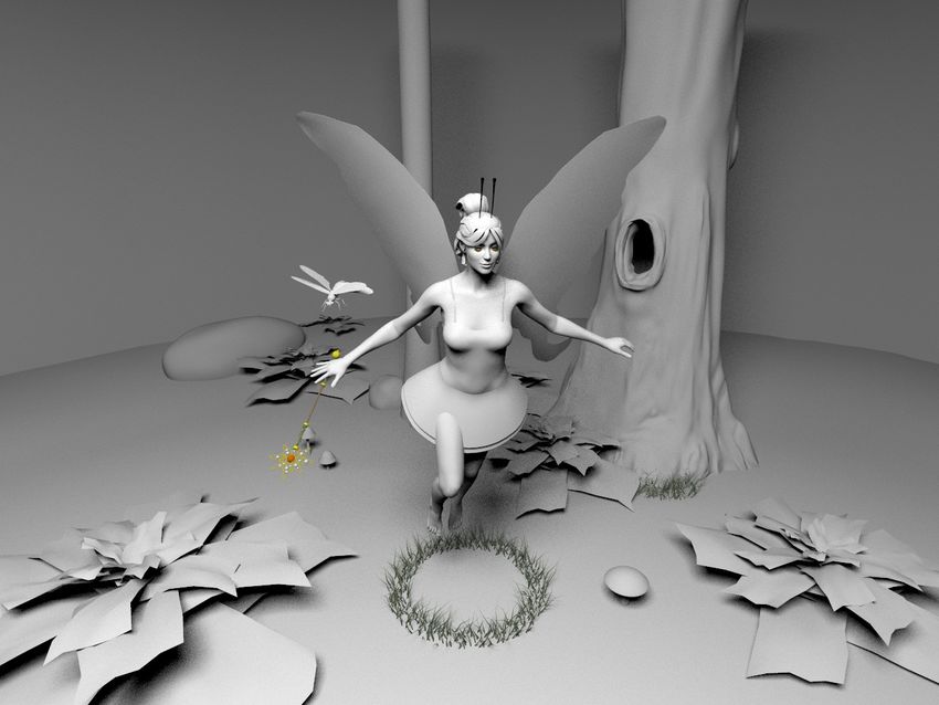
J. Kalojanov, M. Billeter & P. Slusallek / Two-Level Grids for Ray Tracing on GPUs
Reference Algorithm 1 Data-Parallel Two-Level Grid Construction.
Array: 0 C A A B C B C C D C C B B
1 2 3 4 5 6 7 8 9 10 11 12
Kernel calls are suffixed by < >. Scan and sort may con-
Leaf Array: sist of several kernel calls.
b ← COMPUTE BOUNDS ()
[0,0) [0,0) [0,1) [0,0) [1,2) [2,5) [0,0) [0,0) [5,7) [7,8)
2: r ← COMPUTE TOP LEVEL RESOLUTION ()
Top
t ← UPLOAD TRIANGLES ()
Level 4: data ← BUILD UNIFORM GRID (t, b, r)
D
A Cells: 0, 3x3 9,1x1 10,2x2 Atl p ← GET SORTED TOP - LEVEL PAIRS (data)
C
6: n ← GET NUMBER OF TOP - LEVEL REFERENCES (data)
B 14,1x1 15,1x1 16,1x1 tlc ← GET TOP - LEVEL CELL RANGES (data)
8: . C OMPUTE LEAF CELL LOCATIONS
17,1x1 18,1x1 19,1x1
G ← (ry , rz ), B ← rx
10: Acc ← ARRAY OF rx ∗ ry ∗ rz + 1 ZEROES
Acc ← COUNT LEAF CELLS (b, r,tlc)
12: Acc ← EXCLUSIVE SCAN (Acc , rx ∗ ry ∗ rz + 1)
. S ET LEAF CELL LOCATIONS AND CELL RESOLUTION
Figure 1: The two-level grid is represented by the top-level
14: tlc ← INITIALIZE (Acc ,tlc)
cells (bottom right), the leaf array (second line) and the
. C OMPUTE REFERENCE ARRAY SIZE
primitive reference array (top).
16: G ← 128, B ← 256
Arc ← ARRAY OF G + 1 ZEROES
18: Arc ← COUNT LEAF REFS(t, b, r, n, Atl p ,tlc)
to how uniform grids are typically stored [LD08, WIK∗ 06, Arc ← EXCLUSIVE SCAN (Arc , G + 1)
KS09]. 20: m ← Arc [G]
A p ← ALLOCATE LEAF PAIRS ARRAY (m)
Each top-level cell provides the data needed to access its 22: . F ILL REFERENCE ARRAY
sub-cells. Those are the resolution of the grid in this cell as A p ← WRITE PAIRS(t, b, r, n, Atl p ,tlc, Arc )
well as the location of its leaf cells. We store all leaf cells in 24: A p ← SORT (A p )
a single leaf array. lea f s ← EXTRACT CELL RANGES< >(A p , m)
Each leaf cell has to provide the primitives that it overlaps
spatially. We store references to the primitives in a single ref-
erence array. This array has two important properties. First,
each primitive is referenced as many times as the number of
cells it overlaps. Second, references to primitives intersect-
ing the same leaf cell are stored next to each other in the Kalojanov and Slusallek [KS09] reduce the construction
array. Hence for each leaf cell in the grid there is an interval of uniform grids to sorting(Figure 2). There, the reference
in the reference array, and the primitives referenced in this array for the uniform grid is constructed by emitting and
interval are the ones that overlap the cell spatially. sorting pairs of cell index and primitive reference. This algo-
rithm allows for optimal work distribution regardless of the
In our implementation we use two 32-bit values for each
primitive distribution in the scene, but is restricted to con-
cell and each leaf. A leaf stores two integral values that indi-
structing a single uniform grid in parallel.
cate where to find the references to the primitives in the leaf
(see Figure 1). For each top cell we store the location of the For the leaf cells of the two-level grid we need to construct
first leaf cell (32 bits) together with the cell resolution com- multiple uniform grids of various resolution, each contain-
pressed in 24 bits. We leave out 8 bits for flags that denote ing arbitrary number of primitives. Building each of the top-
status like “is empty” or “has children”. Note that using only level cells independently would make the entire construc-
24 bits limits the resolution of each top level cell to 2563 , tion too expensive. The main contribution of this paper is
but this limitation is implementation specific. an efficient algorithm for constructing the entire leaf level
of the two-level grid with a single sort. Our algorithm is a
generalization of the sort-based grid construction proposed
3. Sort-Based Construction
by Kalojanov and Slusallek [KS09] based on the following
We build the two-level grid in a top-down manner. We con- observation: In order to use sorting to construct the entire ar-
struct a uniform grid, which we use to initialize the top-level ray of primitive references for the cells at each level of the
cells. We then construct the reference array for the leaves in structure, we have to select a set of keys that form a one-one
parallel by writing pairs of keys and primitive references in a correspondence with the cells. We take advantage of the fact
random order and sorting them. Finally, we read out the leaf that we store the leaves in a single array, and choose to use
cells from the sorted array of pairs. the memory location of the leaf as key.
c 2010 The Author(s)
Journal compilation c 2010 The Eurographics Association and Blackwell Publishing Ltd.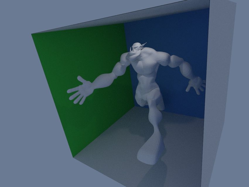
J. Kalojanov, M. Billeter & P. Slusallek / Two-Level Grids for Ray Tracing on GPUs

                                                                                        stant time from its dimensions and the number of primitives
                                                                                        it contains as detailed in Section 5. The resolution also gives
    Input                                                                               the number of leaf cells each top-level cell contains.
                                            (Cell ID, Prim ID)
               A                                                                           We perform a prefix sum over the amount of leaf cells
                             Write            0 A     1 A 2 A         0 B 3 B
      B                      Pairs                                                      for each top-level cell to compute the location of the first
                                                             Radix                      leaf for every top-level cell (lines 9 to 11). After the scan is
                                                             Sort                       performed in line 12, the n-th value of the resulting array is
   Grid Cells                                                                           the position in the leaf array where the first leaf of the n-th
    [0,2) [2,3) [3,4)                                                                   top-level cell is located.
                                              Sorted Pairs
                                 Extract
    [4,5) [0,0) [0,0)            Cells        0 A     0 B    1 A      2 A 3 B

    [0,0) [0,0) [0,0)                                                                   3.2. Writing Unsorted Pairs
                                                                                        Having initialized the data for the top-level cells allows us
                                                                                        to start writing the array of pairs that will later be sorted
                                                                                        and converted to the final array with primitive references.
Figure 2: Sort-based construction of uniform grids. We use                              Because it is not possible to dynamically allocate memory
this algorithm to compute the top-level of the two-level grid.                          on current GPUs we have to compute the size of the array
                                                                                        and allocate it in advance (Lines 16 to 19).
   Input                                 Top Cells                                         In contrast to the construction of the top-level grid, we
                       D
       A
               C                           0, 3x3 9,1x1 10,2x2                          cannot use the leaf index relative to the top cell as a key
                           Build
           B               Top             14,1x1 15,1x1 16,1x1                         to identify primitive-leaf overlaps, as these leaf indices are
                           Cells           17,1x1 18,1x1 19,1x1                         not unique. For example, in Figure 1 there are nine leaves
                                                                                        with index 0 and two with index 1. We want a single sort to
                           0A      0B 0C           1 C 2 C       2D    3 B   4 B
                                                                                        yield the final reference array. To this end we instead use the
                                     Write Pairs
 (Leaf Location, Prim ID)
                                                                                        location of the cell in the leaf array with the primitive index.
 4 A 5 A 5 B 8 B 2 C 5 C 8 C 9 C 12 C 13 C 11 D 14 B 15 B
                                                                                        This location is easy to compute from the leaf index and the
                                                                                        location of the first leaf for the corresponding top-level cell,
                                     Radix Sort
 Sorted Pairs                                                                           which we already have.
 2 C 4 A 5 A 5 B 5 C 8 B 8 C 9 C 11 D 12 C 13 C 14 B 15 B                                  We use a fast but conservative triangle-cell intersection
                                   Extract Leaves                                       test when counting the output pairs and a more precise but
                                                                                        slower one when generating them. First we only consider the
[0,0) [0,0) [0,1) [0,0) [1,2) [2,5) [0,0) [0,0) [5,7) [7,8) [0,0) [8,9)                 bounding box of the triangle, and later we also make sure
                                                                                        that the plane in which the triangle lies intersects the cell.
Figure 3: Two-level grid construction. When we construct                                The invalid intersections are still written with a dummy cell
the top-level, we use cell indices as keys. The second set of                           index that is discarded in the sorting stage.
pairs uses the memory location of the leaf cell as key. After
being sorted, the leaf pairs yield the reference array (not in
the figure) and the leaf cells.                                                         3.3. Sorting the Pairs
                                                                                        The order of the primitive references in the sorted array is
                                                                                        the same as in the final reference array. We use an improved
                                                                                        version of the radix sort by Billeter et al. [BOA09], which
3.1. Building the Top-Level Cells
                                                                                        uses a combination of two- and four-way splits. The size of
To construct the top-level cells, we build a uniform grid us-                           the largest key we need to sort is known, which tells us the
ing the sorting-based approach by Kalojanov and Slusallek                               number of bits that need to be considered. We sort only on
[KS09]. The algorithm amounts to determining all triangle-                              the required bits, up to two bits at a time.
cell overlaps and storing the information as an array of pairs.
As illustrated in Figure 2, this intermediate data is sorted us-
                                                                                        3.4. Extracting the Leaf Cells
ing the cell indices as keys.
                                                                                        In the final stage of the construction algorithm, we com-
   A notable modification of the original approach is that we
                                                                                        pute the leaf cells directly from the sorted array of pairs.
keep the sorted array of pairs (see line 5 of Algorithm 1) and
                                                                                        We check in parallel for range borders, i.e. neighboring pairs
use it as input for the next stages of the construction instead
                                                                                        with different keys (e.g. the second and third sorted pairs in
of the original set of input primitives.
                                                                                        Figure 3). To be able to access the primitives inside each
   The resolution of each top-level cell is computed in con-                            cell in constant time during rendering, we store the start and

 c 2010 The Author(s)
Journal compilation c 2010 The Eurographics Association and Blackwell Publishing Ltd.
J. Kalojanov, M. Billeter & P. Slusallek / Two-Level Grids for Ray Tracing on GPUs
this holds only if there are enough input primitives, which is
Thai Statue 77 53 86 13
almost always the case. This is possible because in each step
Soda Hall 16 14 24 4 threads are mapped to tasks independently. In addition to the
high parallelism, the runtime is independent of the primitive
Conference 3 5.5 7 1
distribution in the scene exactly like the sort-based uniform
Exploding grid construction [KS09].
3 2 3 1
Dragon 6
Fairy 0 3 1 3 1
4.2. Memory Footprint
0% 20% 40% 60% 80% 100%
In terms of memory footprint, the two-level grids consume
Build Top Level Write Pairs Radix Sort Extract Grid Cells less memory mainly because of the reduced amount of cells
compared to a single-level uniform grid. The main memory
bottleneck here is the space required to store the references.
Because the two-level grids are more memory friendly than
uniform grids, we were able to construct the acceleration
structure for models such as the Thai Statue, which consists
Figure 4: Times for the different stages of the build algo-
of 10 million triangles, on a graphics card with 1GB of mem-
rithm in milliseconds. The complete runtime is the sum of the
ory.
measured values. Exploding Dragon 6 and Fairy 0 means
that the seventh and first frame from the animations were
measured. Times are measured on a GTX 285. 5. Grid Resolution
Our choice of grid resolution is based on the heuristic for
uniform grids introduced by Cleary et al. [CWVB83] and
end of each range inside the corresponding leaf cell. This is also used by Wald et al. [WIK∗ 06]:
straight-forward to do, since we can read the location of the r r r
3 λN 3 λN 3 λN
cell from the key we used for sorting the pairs. After we out- Rx = dx , Ry = dy , Rz = dz , (1)
put the leaf array, we extract the reference array out of the V V V
pairs array to compact the data and free space. where d~ is the extent of the box in all dimensions and V is
the volume of the scene’s bounding box. N is the number of
4. Analysis primitives, and λ is a user-defined constant called grid den-
sity. Thus the number of cells is a multiple of the input prim-
Apart from being fast, the most important feature of the con- itives. Ize et al. [ISP07] investigate optimal grid densities
struction algorithm is that its work complexity is linear. This for uniform and two-level grids. The best densities for CPU
is one of the reasons to prefer radix sort, another one is ray tracing suggested by the authors proved sub-optimal for
the availability of a fast GPU implementation by Billeter et our GPU ray tracer. Ize et al. base their theoretical analysis
al. [BOA09]. Note that the data we have is well suited for on several assumptions including fast atomic operations and
bucket sort algorithms like radix sort because the range of compute limited traversal, which did not hold for the hard-
different key values is small compared to the input size. The ware we used. Additionally Popov et al. [PGDS09] demon-
complexity would not be linear if we were not able to deter- strate that for other acceleration structures like BVHs treat-
mine the cell resolution in constant time, knowing the num- ing the geometric primitives as points can severely limit the
ber of overlapped primitives and the extent of the bounding quality.
box of each top-level cell.
To find optimal grid densities and work around the issues
mentioned above we employ the Surface Area Metric, in-
4.1. Runtime troduced by MacDonald and Booth [MB90], to compute the
The runtime is more or less equally distributed between the expected cost (Ce ) for traversing a random ray through the
different stages of the construction (see Figure 4). The most acceleration structure:
time-consuming stages of the algorithm – writing the pairs Ce = Ct Pr(n) +Ci Pr(l)Prim(l), (2)
and sorting them – are memory bandwidth limited. We do
∑ ∑
n∈Nodes l∈Leaves
not require any synchronization inside the kernels. Atomic
where Ct and Ci are constant costs for traversing a node of
synchronization is not necessary, but we use atomic incre-
the structure and intersecting a geometric primitive, Pr(·) is
ment on shared memory for convenience when writing pairs
the probability of a random line intersecting a node or leaf,
in the unsorted array.
and Prim(·) is the number of geometric primitives in a leaf
The algorithm is able to exploit the high parallelism of node. In our case the nodes of the structure are the grid cells
modern GPUs because the work is evenly distributed among and computing the cost for a particular grid density amounts
as many threads as the hardware is able to manage. Of course to constructing the top level of the grid and counting the
c 2010 The Author(s)
Journal compilation c 2010 The Eurographics Association and Blackwell Publishing Ltd.J. Kalojanov, M. Billeter & P. Slusallek / Two-Level Grids for Ray Tracing on GPUs
Soda Venice Conf. Dragon Fairy Sponza sal to spare computations when initializing the decision vari-
Ct = 1 12 2.4 2.1 1.4 1.9 1.4 2.1 ables for the leaf level.
Ct = 2 1.8 1.8 1.3 1.4 0.9 1.6
Ct = 3 1.2 1.2 1.3 1.0 0.9 1.3 The traversal algorithm has properties similar to the uni-
form grid traversal. It is SIMD (or SIMT) friendly since
Table 1: Optimal densities λ for the leaf level of the grid there is no code divergence, except when the rays disagree
computed according to the cost model based on the Surface on which level of structure they need to traverse. The algo-
Area Metric. Cost for intersection was 1 for all listed traver- rithm favors coherent rays. In the case of uniform grids, one
1
sal costs (Ct ). The first level ot the grid had λ = 16 can easily show that for rays starting in the same grid cell
will traverse every cell of the grid at exactly the same step of
the DDA traversal algorithm:
Statement:Let Ro be a set of rays, all of which have origin
primitives referenced in the leaves, which is easily done af- (not necessarily the same) in a given grid cell o. If a cell c is
ter slight modification of the initial stage of our construction intersected by any ray r ∈ Ro and is the n-th cell along r
algorithm – the kernel that counts the fragments in the leaf counted from the origin, then c will be n-th cell along any
level of the grid. ray r2 ∈ Ro that intersects c.
1
We set the top level density to λ = 16 to make better use
of our hybrid intersector, which is explained in detail later Proof: Let o be the 0-th cell along the rays in the set. For
in Section 7 and benefits from cells that contain at least 16 each cell c holds that it is at distance (x, y, z) from o, where
primitives. Then we tested our traverser and intersector per- x, y and z are integers and each denotes the distance (in
formance separately and together on an artificially created number of cells) along the coordinate axis with the same
grid with various number of primitives per cell. We took the name. During traversal, the rays advance with exactly one
ratios of empty to full leaf cells from our test scenes. Our ray neighbor cell at a time and the two cells share a side. This
tracing implementation performed best on relatively sparse means that c will be traversed at x + y + z = n-th step of the
grids when we did 1 12 intersection tests per traversal step. traversal algorithm for any ray with origin in o if at all.
Thus we tried Ct = 1 12 , 2, 3 and Ci = 1 looking for close to
This means that a cell along the traversal path, if loaded,
optimal rendering performance and sparse grid resolutions
will be loaded exactly once from memory. This property
that would allow faster construction and the best time to im-
transfers to the two-level grid structure when traversing the
age for dynamic scenes. Given the costs for traversal and in-
1 top level and when rays agree on the first leaf cell when they
tersections we tested all grid densities starting with 16 , and
1
traverse the leaves.
adding 16 until we reached λ = 8. The densities with optimal
costs for some of our test scenes are listed in Table 1.
7. Triangle Intersection
While the optimal density for the two-level grid is scene
dependent, the rendering performance for all scenes did not During the ray-triangle intersection stage of the ray traversal
vary noticeably for values of λ between 12 and 2. In the re- the coherence in the computations executed by the different
mainder of the paper the density of each top-level cell is set threads is lost as soon as some of the rays traverse a full cell,
to λ = 1.2. Note that we use a global value for λ across all while others pass through an empty one. This is the case
top-level cells. Choosing the different density or even differ- because we parallelize by assigning different rays to each
ent resolution for different top level cells can provide higher thread, which ties SIMD efficiency to ray coherence. The
quality grids, but would make the construction too slow as two-level grids we use for rendering are sparse compared to
already observed by Kalojanov and Slusallek [KS09]. Also other acceleration structures and contain more primitives per
note that we used the Surface Area Cost Model to determine leaf. We exploit this property and distribute work for a sin-
a single grid density that works well with our traversal im- gle ray to many threads to speed up traversal by improving
plementation for all test scenes. SIMD utilization.
We employ a hybrid packetization strategy during ray-
triangle intersection. In each warp (SIMD unit consisting
6. Ray Traversal
of 32 threads), we check if all rays have intersection candi-
Similar to the uniform grids, the traversal of two-level grids dates and if this is the case we proceed with the standard ray-
is very inexpensive. We modified the DDA traversal algo- triangle intersection. If this is not the case, we check if there
rithm by Amanatides and Woo [AW87]. We step through the are rays with high workload - at least 16 intersection candi-
top level of the structure as we would do for a uniform grid. dates. If these are more than 20 we proceed with the standard
We treat each top cell as a uniform grid itself and use the intersection routine. This part of the algorithm maps better to
same algorithm to advance through the leaf cells. One can Fermi GPUs, because they support more Boolean operations
reuse some of the decision variables for the top-level traver- on warp level in hardware.
c 2010 The Author(s)
Journal compilation c 2010 The Eurographics Association and Blackwell Publishing Ltd.J. Kalojanov, M. Billeter & P. Slusallek / Two-Level Grids for Ray Tracing on GPUs
Scene Tris Refs Top Leaf MB Time Model LBVH H BVH Grid 2lvl Grid
Thai 10M 27.2M 226K 11.8M 194 257 Fairy 10ms 124ms 24ms 8ms
Soda 2.2M 6.6M 48K 1.4M 52 67 (174K) 1.8 fps 11.6 fps 3.5 fps 9.2 fps
Venice 1.2M 3.7M 27K 1.5M 26 32 Conference 19ms 105ms 27ms 17ms
Conference 284K 2.3M 6K 358K 10 17 (284K) 6.7 fps 22.9 fps 7.0 fps 12.0 fps
Dragon 252K 905K 5K 307K 5 10 Expl. Dragon 17ms 66ms 13ms 10ms
Fairy 174K 514K 3K 206K 4 8 (252K) 7.3 fps 7.6 fps 7.7 fps 10.3 fps
Soda Hall 66ms 445ms 130ms 67ms
Table 2: Build statistics with density of each top-level cell (2.2M) 3.0 fps 20.7 fps 6.3 fps 12.6 fps
λ = 1.2. Refs is the number of primitive references in the
final structure. Top and Leaf are amount of top-level and Table 3: Build times and frame rates (excluding build time)
leaf cells. MB is the amount of memory (in MB) required to for primary rays and dot-normal shading for a 1024 × 1024
store all cells and the references. Times (in ms) are measured image. We compare our non-optimized implementation to the
on a GTX 285. We used the second frame of the Exploding results of Lauterbach et al. [LGS∗ 09] and Kalojanov and
Dragon animation, and the sixth frame of the Fairy Forest Slusallek [KS09]. The Hybrid BVH (H BVH) [LGS∗ 09] is a
animation. BVH with close to optimal expected cost for traversal. All
times are measured on a GTX 280.
8.1. Construction
If we have determined that standard packetization would We give the performance of our implementation in Table 2.
be inefficient and there are rays with high workload, we in- We include all overheads except the initial upload of the
sert those into a buffer in shared memory. This is done with scene primitives to the GPU. The runtime grows with the
an atomic increment on a shared counter. We only need to number of pairs (i.e. number of primitive references), which
store the index of the ray and the first intersection candidate, is scene dependent. The measured frames from the Explod-
because the indices of the remaining primitives are consec- ing Dragon and Fairy Forest animations are the worst case
utive. We iterate on the entries of this buffer taking two at examples for the build performance during the animations.
a time and perform 32 intersection tests for a pair of rays
in parallel. We combine the results by performing reduction Note that the number of primitive references required for
on the arrays with the intersection distances, which are also rendering is smaller than the total number of references. This
shared between threads. Finally, the thread responsible for is the case because we use the sorting stage to discard cell-
tracing the ray records the closest intersection (if there is triangle pairs that were generated using a more conservative
one) in thread local memory. When all rays with high work- triangle insertion test.
load have been processed we perform the remaining inter- Pantaleoni and Luebke [PL10] improve on the LBVH
section tests one by one for all rays as usual. construction algorithm proposed by Lauterbach et al.
[LGS∗ 09] and achieve superior build performance and scal-
We chose to define 16 intersection candidates as high
ability for their HLBVHs. To our knowledge the HLBVH
workload, since the actual SIMD width of 32 was too big
is the structure that is fastest to construct on modern GPUs.
and in our structure there were not many cells with enough
The test results in Table 2 suggest that our algorithm also
primitives. Having to process more than 2 rays at a time on
scales very well with scene size. The build times for the two-
the other hand turned out to introduce too much overhead.
level grids depend on the chosen density and the primitive
To derive the last parameter – the number (20) of active rays
distribution – we need around 10 ms per 1 million refer-
above which horizontal parallelization does not pay off – we
ences. For densities around 1, which proved to be optimal
benchmarked the speed of our implementation with all pos-
for our renderer, construction times were close to and some-
sible numbers of active rays.
times faster than those of Pantaleoni and Luebke.
8.2. Rendering
8. Results
We tested the build and render times for the two-level grid
We implemented the two-level grid builder together with a in Table 3. We clearly see that the new structure han-
GPU ray tracer in CUDA. We tested performance on a ma- dles a teapot in the stadium scene like the Fairy Forest
chine with an NVIDIA GeForce GTX 285, GTX 280, or a much better than uniform grids. Here we did not include
GTX 470 and an Intel Core 2 Quad processor running at 2.66 persistent threads - an optimization proposed by Aila and
GHz. The CPU performance is almost irrelevant for the re- Laine [AL09], that deals with a drawback of the GT200-
sults since we only use it to schedule work and transfer data class NVIDIA GPUs related to work distribution. We did
to the graphics card. this with the purpose to allow a fair comparison, at least to
c 2010 The Author(s)
Journal compilation c 2010 The Eurographics Association and Blackwell Publishing Ltd.J. Kalojanov, M. Billeter & P. Slusallek / Two-Level Grids for Ray Tracing on GPUs
Ogre Fairy Conf. Venice sistent threads [AL09]. Thus we did not use it when testing
(50K) (174K) (284K) (2.2M) on the GTX285. Fermi GPUs (e.g. the GTX 470) have hard-
GTX 285 ware support for population count and prefix sum on warp
Dot-Normal 31 fps 15 fps 22 fps 18 fps level which allows to implement the intersector more effi-
Direct Illumination 7.8 fps 2.7 fps 3.0 fps 3.3 fps ciently. We used the hybrid intersector together with persis-
Path Tracing 3.4 fps 2.1 fps 1.6 fps 1.4 fps tent threads on the newer Fermi GPUs, which improved the
GTX 470 Hybrid overall performance of our path tracer. The improvement in-
Dot-Normal 44 fps 22 fps 27 fps 26 fps
creased when rendering smaller resolution windows, which
Direct Illumination 10 fps 4.6 fps 3.7 fps 4.7 fps
reduces ray coherency, but the overall performance gain due
Path Tracing 4.7 fps 2.8 fps 2.4 fps 2.3 fps
to the hybrid intersector did not exceed 10%. Although the
GTX 470 Simple
gain is not big, it is interesting to see that such hybrid par-
Dot-Normal 46 fps 21 fps 26 fps 24 fps
Direct Illumination 10 fps 3.7 fps 3.3 fps 4.5 fps
allelization scheme can work in practice. This indicates that
Path Tracing 4.7 fps 2.6 fps 2.4 fps 2.1 fps control flow divergence can limit the performance on wide
SIMD machines and adding some computational overhead
Table 4: Frame rate (in frames per second) for rendering a to reduce it can pay off on future hardware.
1024 × 1024 image on a GTX 285, GTX 470 with our hybrid
Overall, the traversal performance provided by two-level
intersector and without it. We measure the time required to
grids is not as high as state-of-the-art approaches for static
generate an image with dot-normal shading (1 primary ray
scenes. We implemented the test setup described by Aila
per pixel), diffuse shading and direct illumination from an
and Laine [AL09]. We were able to trace 24 and 22 million
area light source (1 primary and 4 shadow rays), and path
primary rays per second for the Conference and the Fairy
tracing with 3 rays per pixel on average. This implementa-
scene compared to 142 and 75 million as reported by Aila
tion includes persistent threads. The frame rates for the Ogre
and Laine. We used the viewports in Figure 5. In terms of
and Fairy scenes include rebuild of the grid for each frame.
traversal performance, the two-level grids are comparable to
other acceleration structures that are fast to construct like the
LBVH or the Hybrid BVH, but our approach offers inferior
some extent, as neither Lauterbach et al. nor Kalojanov and performance to algorithms optimized for static geometry.
Slusallek used this optimization. In Table 4, we give frame
rates of the same implementation after we added persistent
threads.
Since primary rays are very coherent and maybe the 9. Discussion and Future Work
fastest to traverse, we also evaluated the traversal perfor-
There are various possible continuations of this work. Since
mance of other types of rays as well. In Table 4 we test per-
the main drawback of our approach is the ray traversal per-
formance on two dynamic and two static scenes. We com-
formance, it will be interesting to investigate whether or not
pare the performance for dot-normal shading with an imple-
different traversal algorithms can map better to the hardware
mentation of diffuse direct illumination from an area light
architecture and provide faster rendering times.
source. For the latter, we trace 4 shadow rays starting at each
hit point and ending in a uniformly sampled random point The sort-based construction algorithm can be extended to
on the light source. build hierarchies with arbitrary depth. The tree has to be
The last scenario we tested in Table 4 is path tracing constructed top-down and breadth-first. At each level d one
diffuse surfaces. We terminate the paths based on Russian needs to identify a unique index of every node with depth
Roulette with probability 12 and shoot a single shadow ray at d + 1. The index can be paired with the indices of the over-
the end of each path to compute the direct contribution from lapping primitives. After the pairs are sorted, the tree nodes
the area light source previously used for the direct illumina- of depth d + 1 can be read out from the sorted array. Hierar-
tion test. We do not shoot other shadow rays except the one chical grids with depth larger than two might offer better ac-
at the end of the path and generate secondary ray directions celeration for ray tracing on future hardware. Extending our
with cosine distribution around the surface normal. Note that traversal implementation to three-level grids did not make
this benchmark produces very incoherent rays and the SIMD sense, because of the increased amount of registers required
units are under-utilized because of ray termination. For each to run the code.
sample per pixel the average number of rays is 3, the longest
A variant of the algorithm can be used to construct mul-
path has length 15, and the warps stay active for 6 bounces
tiple uniform grids over different objects in parallel. This
on average for the test scenes.
requires almost no modifications of the current implementa-
On GT200 class GPUs, the hybrid ray-triangle intersec- tion. The construction of the leaf level of the two-level grid
tion (Section 7) improved the overall performance for inco- in fact performs this task, where the grids are actually cells
herent rays by up to 25%, but only if we did not use per- of the top level of the structure.
c 2010 The Author(s)
Journal compilation c 2010 The Eurographics Association and Blackwell Publishing Ltd.J. Kalojanov, M. Billeter & P. Slusallek / Two-Level Grids for Ray Tracing on GPUs
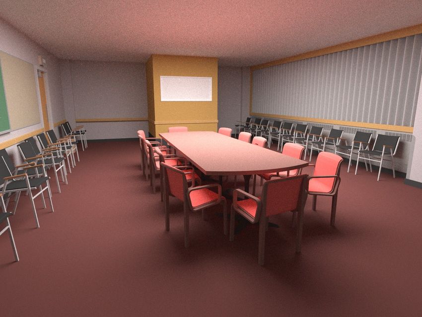
Figure 5: Some of our test scenes, from left to right - Ogre, Fairy Forest, Exploding Dragon and Conference. The images were
rendered using path tracing, diffuse direct illumination, dot-normal shading and path tracing respectively.
10. Conclusion [ISP07] I ZE T., S HIRLEY P., PARKER S.: Grid creation strategies
for efficient ray tracing. Symposium on Interactive Ray Tracing
The acceleration structure discussed in this paper is a sim- (Sept. 2007), 27–32. 4
ple extension of the uniform grid that copes better with non- [JW89] J EVANS D., W YVILL B.: Adaptive voxel subdivision
uniform triangle distributions. Our goal was to both improve for ray tracing. In Proceedings of Graphics Interface ’89 (June
the quality of the acceleration structure and maintain the fast 1989), Canadian Information Processing Society, pp. 164–72. 1
build times. For our tests scenes, the rendering performance [KS09] K ALOJANOV J., S LUSALLEK P.: A parallel algorithm
increased overall, and especially when rendering parts of the for construction of uniform grids. In HPG ’09: Proceedings of
scene with more complex geometry. The build times of the the 1st ACM conference on High Performance Graphics (2009),
two-level grids are comparable and in general lower than ACM, pp. 23–28. 1, 2, 3, 4, 5, 6
those of uniform grids when using resolutions optimal for [LD08] L AGAE A., D UTRÉ P.: Compact, fast and robust grids
rendering in both cases. To our knowledge, there is no ac- for ray tracing. Computer Graphics Forum (Proceedings of the
19th Eurographics Symposium on Rendering) 27, 4 (June 2008),
celeration structure that is significantly faster to construct on 1235–1244. 2
modern GPUs. We believe that this and the reasonable ren-
[LGS∗ 09] L AUTERBACH C., G ARLAND M., S ENGUPTA S.,
dering performance makes the two-level grid a choice worth L UEBKE D., M ANOCHA D.: Fast BVH construction on GPUs.
considering for ray tracing dynamic scenes. We also hope In Proceedings of Eurographics (2009). 1, 6
that the general ideas for the parallel construction and the [MB90] M AC D ONALD J. D., B OOTH K. S.: Heuristics for ray
hybrid packetization can be adapted and used in different tracing using space subdivision. Visual Computer 6, 6 (1990),
scenarios, e.g. with different spatial index structures. 153–65. 1, 4
[NBGS08] N ICKOLLS J., B UCK I., G ARLAND M., S KARDON
K.: Scalable parallel programming with CUDA. In Queue 6.
Acknowledgements ACM Press, 2 2008, pp. 40–53. 1
The models of the Dragon and the Thai Statue are from The [PGDS09] P OPOV S., G EORGIEV I., D IMOV R., S LUSALLEK
Stanford 3D Scanning Repository, the Bunny/Dragon and P.: Object partitioning considered harmful: space subdivision for
the Fairy Forest Animation are from The Utah 3D Animation bvhs. In HPG ’09: Proceedings of the 1st ACM conference on
High Performance Graphics (2009), ACM, pp. 15–22. 4
Repository. We would like to thank the anonymous review-
ers and Vincent Pegoraro for the suggestions which helped [PL10] PANTALEONI J., L UEBKE D.: HLBVH: Hierarchical
LBVH Construction for Real-Time Ray Tracing. In High Per-
improving the quality of this paper. formance Graphics (2010). 1, 6
[Wal10] WALD I.: Fast Construction of SAH BVHs on the Intel
References Many Integrated Core (MIC) Architecture. IEEE Transactions
on Visualization and Computer Graphics (2010). (to appear). 1
[AL09] A ILA T., L AINE S.: Understanding the efficiency of ray
traversal on GPUs. In HPG ’09: Proceedings of the 1st ACM con- [WIK∗ 06] WALD I., I ZE T., K ENSLER A., K NOLL A., PARKER
ference on High Performance Graphics (2009), ACM, pp. 145– S. G.: Ray tracing animated scenes using coherent grid traversal.
149. 6, 7 ACM Transactions on Graphics 25, 3 (2006), 485–493. 2, 4
[AW87] A MANATIDES J., W OO A.: A fast voxel traversal al- [WMG∗ 07] WALD I., M ARK W. R., G ÜNTHER J., B OULOS S.,
gorithm for ray tracing. In Eurographics ’87. Elsevier Science I ZE T., H UNT W., PARKER S. G., S HIRLEY P.: State of the Art
Publishers, 1987, pp. 3–10. 5 in Ray Tracing Animated Scenes. In Eurographics 2007 State of
the Art Reports (2007). 1
[BOA09] B ILLETER M., O LSSON O., A SSARSSON U.: Efficient
stream compaction on wide SIMD many-core architectures. In [ZHWG08] Z HOU K., H OU Q., WANG R., G UO B.: Real-time
HPG ’09: Proceedings of the Conference on High Performance kd-tree construction on graphics hardware. In SIGGRAPH Asia
Graphics 2009 (2009), ACM, pp. 159–166. 3, 4 ’08: ACM SIGGRAPH Asia 2008 papers (2008), ACM, pp. 1–11.
1
[CWVB83] C LEARY J. G., W YVILL B. M., VATTI R.,
B IRTWISTLE G. M.: Design and analysis of a parallel ray tracing
computer. In Graphics Interface ’83 (1983), pp. 33–38. 4
c 2010 The Author(s)
Journal compilation c 2010 The Eurographics Association and Blackwell Publishing Ltd.You can also read