Two MODIS Aerosol Products over Ocean on the Terra and Aqua CERES SSF Datasets
←
→
Page content transcription
If your browser does not render page correctly, please read the page content below
1008 JOURNAL OF THE ATMOSPHERIC SCIENCES—SPECIAL SECTION VOLUME 62
Two MODIS Aerosol Products over Ocean on the Terra and Aqua CERES SSF
Datasets
ALEXANDER IGNATOV,* PATRICK MINNIS,⫹ NORMAN LOEB,# BRUCE WIELICKI,⫹ WALTER MILLER,@
SUNNY SUN-MACK,@ DIDIER TANRÉ,& LORRAINE REMER,** ISTVAN LASZLO,* AND ERIKA GEIER⫹
* NOAA/NESDIS/Office of Research and Applications, Camp Springs, Maryland
⫹ Atmospheric Sciences, NASA Langley Research Center, Hampton, Virginia
# Center for Atmospheric Sciences, Hampton University, Hampton, Virginia
@ Science Applications International Corporation, Hampton, Virginia
& Laboratoire d’Optique Atmospherique, Universite des Sciences et Technologies de Lille, Villenueve d’Asq, France
** NASA Goddard Space Flight Center, Greenbelt, Maryland
(Manuscript received 8 August 2003, in final form 25 June 2004)
ABSTRACT
Understanding the impact of aerosols on the earth’s radiation budget and the long-term climate record
requires consistent measurements of aerosol properties and radiative fluxes. The Clouds and the Earth’s
Radiant Energy System (CERES) Science Team combines satellite-based retrievals of aerosols, clouds, and
radiative fluxes into Single Scanner Footprint (SSF) datasets from the Terra and Aqua satellites. Over
ocean, two aerosol products are derived from the Moderate Resolution Imaging Spectroradiometer
(MODIS) using different sampling and aerosol algorithms. The primary, or M, product is taken from the
standard multispectral aerosol product developed by the MODIS aerosol group while a simpler, secondary
[Advanced Very High Resolution Radiometer (AVHRR) like], or A, product is derived by the CERES
Science Team using a different cloud clearing method and a single-channel aerosol algorithm. Two aerosol
optical depths (AOD), A1 and A2, are derived from MODIS bands 1 (0.644 m) and 6 (1.632 m)
resembling the AVHRR/3 channels 1 and 3A, respectively. On Aqua the retrievals are made in band 7
(2.119 m) because of poor quality data from band 6. The respective Ångström exponents can be derived
from the values of . The A product serves as a backup for the M product. More importantly, the overlap
of these aerosol products is essential for placing the 20⫹ year heritage AVHRR aerosol record in the
context of more advanced aerosol sensors and algorithms such as that used for the M product.
This study documents the M and A products, highlighting their CERES SSF specifics. Based on 2 weeks
of global Terra data, coincident M and A AODs are found to be strongly correlated in both bands.
However, both domains in which the M and A aerosols are available, and the respective /␣ statistics
significantly differ because of discrepancies in sampling due to differences in cloud and sun-glint screening.
In both aerosol products, correlation is observed between the retrieved aerosol parameters (/␣) and
ambient cloud amount, with the dependence in the M product being more pronounced than in the A
product.
1. Introduction (Wielicki et al. 1996). The TRMM satellite carries the
CERES protoflight model (PFM); Terra carries flight
Aerosols have an important, yet somewhat uncertain, models 1 and 2 (FM1–2); and Aqua carries flight mod-
impact on the earth’s radiation budget and climate. De- els 3 and 4 (FM3–4). The Single Scanner Footprint
termining that impact on the climate record requires (SSF) products (Geier et al. 2003) combine the CERES
consistent measurements of aerosol properties and ra- data with cloud and aerosol retrievals from the Visible
diative fluxes. To that end, three satellites, the Tropical and Infrared Scanner (VIRS) on TRMM and the Mod-
Rainfall Measuring Mission (TRMM), Terra, and Aqua erate Resolution Imaging Spectroradiometer (MODIS)
(launched in November 1997, December 1999, and May on Terra and Aqua. The spatial resolution is ⬃2 km at
2002, respectively), carry a total of five Clouds and the nadir for VIRS, and 0.25–1 km for MODIS. The SSF
Earth’s Radiant Energy System (CERES) instruments retains the mean and standard deviation of the imager
to measure the radiant energy exchange on Earth pixel radiances and cloud/aerosol retrievals separately
for the clear and cloudy portions of every CERES field
of view (FOV). The spatial resolution for CERES
Corresponding author address: Dr. Alex Ignatov, E/RA1, Rm. (equivalent diameter at nadir) is ⬃10 km on TRMM
603, 5200 Auth Road, Camp Springs, MD 20746-4304. and ⬃20 km on Terra and Aqua. Aerosol retrievals on
E-mail: Alex.Ignatov@noaa.gov the SSF have proven useful for a number of applica-
APRIL 2005 IGNATOV ET AL. 1009
tions, such as estimating the surface and atmospheric different radiometric performance of the sensors, or
radiation balance (Charlock et al. 2002) and studies on both.
top-of-atmosphere (TOA) aerosol radiative forcing The availability of the two aerosol products on the
(Loeb and Kato 2002) and molecular albedo (Kato et CERES SSF side by side is helpful to place long-term
al. 2002). time series of the heritage A products from NOAA/
This study documents two aerosol products available AVHRR (20⫹ yr) and TRMM/VIRS (6⫹ yr) in the
over ocean on the Terra and Aqua CERES SSFs and context of more accurate M-aerosol retrievals, and to
compares them using 2 weeks of global Terra data from quickly assess the improvements provided by the mul-
15–21 December 2000 and 1–7 June 2001 (hereafter tichannel MODIS. Ultimately, these analyses provide a
December 2000 and June 2001). Note that the Aqua useful insight into the current status of aerosol retriev-
CERES SSF data are also documented here, but they als from space and serve to highlight and prioritize out-
were not available for science analyses at the time of standing issues.
this writing. The TRMM CERES SSF contains only
one aerosol product based on VIRS data and is ana-
lyzed elsewhere (A. Ignatov et al. 2005, unpublished 2. M- and A-aerosol production over ocean on the
manuscript). Terra and Aqua CERES SSFs
The primary, M, aerosol product on the CERES SSF The first step of the SSF processing includes subsam-
is generated by subsetting and remapping the MOD04 pling of MODIS pixels (nominal resolution at nadir ⬃1
(Terra; MYD04 on Aqua) granules onto CERES foot- km). On the Terra CERES SSF Edition 1A (used in
prints. The MOD04 product uses sophisticated cloud this study), every other pixel/line is sampled, effectively
screening and aerosol retrieval algorithms developed reducing the data volume by a factor of 4. [In the latest
by the MODIS cloud and aerosol groups1 (Tanré et al. version of the SSF software, used in generation of Terra
1997; Ackerman et al. 1998; Martins et al. 2002; Remer Edition 2 and Aqua Edition 1, every fourth (4) pixel in
et al. 2005, hereafter REM). In this study, only two M every other (2) line is subsampled, thereby reducing the
aerosol optical depths, M1 and M2, are used at the data volume by a factor of 8.] The second step is as-
centroid wavelengths of MODIS bands 1 (1⫽0.644 signing aerosol properties from both the MOD04 and A
m) and 6 (2⫽1.632 m). On Aqua, AOD in band 7 products (when available) to the respective subsampled
(2⫽2.119 m) is used for M2 due to poor quality of MODIS pixels. The third step is convolving these sub-
band 6 (C. Moeller 2003, personal communication). sampled pixel aerosol properties into the corresponding
The respective Ångström exponent is derived as ␣M ⫽ CERES footprint using the CERES point spread func-
⫺ln(M1/M2)/ln(1/2). tion (Geier et al. 2003), to provide an optimal match
The secondary A product uses complex, but differ- between the radiative fluxes and aerosol information.
ent, glint and cloud screening criteria and a simpler The CERES SSF aerosol processing is succinctly
[Advanced Very High Resolution Radiometer summarized in Table 1. Note that both M and A prod-
(AVHRR)-like] third-generation aerosol algorithm ucts are reported only at solar zenith angles o⬍70°.
(Ignatov and Stowe 2002a; Ignatov et al. 2004). Two Below, only brief explanations are given. For detail, the
AODs, A1(0.630 m) and A2(1.610 m) [A2(2.119 reader is advised to check with the references cited
m) on Aqua], are derived from MODIS bands 1 and 6 throughout this section and in Table 1.
(7 on Aqua) using single-channel algorithms and re-
ported at the wavelengths representative of band cen-
a. M processing
ters for a generic AVHRR or VIRS sensor. Using a
standard set of reference wavelengths ensures compat- Of the 47 MOD04 ocean and land aerosol param-
ibility of the respective A products derived from a va- eters, 13 ocean and 11 land aerosol parameters are first
riety of sensors (AVHRR, VIRS, and MODIS) flown selected. The selected parameters are then spread to
on board different platforms [National Oceanic and At- each subsampled MODIS pixel found within the
mospheric Administration (NOAA), TRMM, Terra, MOD04 granule (with nominal resolution at nadir 10
and Aqua]. Cross-platform differences in the A prod- km). Finally, all subsampled MODIS pixels are aver-
ucts, if observed, are then due to either different sam- aged into CERES footprints (with nominal resolution
pling of aerosol pixels (specified by domain of sun- at nadir ⬃20 km) and weighted by the CERES point
view-scatter-glint geometry, resulting from the plat- spread function. This convolved average of the MOD04
form’s orbital configuration, and cloud/glint screening), parameters in each SSF constitutes the M product.
The MOD04 processing (Tanré et al. 1997; REM) at
the NASA Goddard Space Flight Center (GSFC) Dis-
1
tributed Active Archive Center is performed in groups
MOD04 processing evolves continuously. Collection 003 was of 20 ⫻ 20 MODIS geolocated pixel reflectances, EV
used in the Terra SSF Edition 1A product analyzed in this study.
As of the time of this revision, Terra Edition 2 and Aqua Edition
o (see appendix A for definitions) at a nominal 500-m
1 CERES SSF products became available based on collection 004 resolution, each cluster resulting in one MOD04 gran-
data, and development of collection 005 is underway. ule. The MODIS aerosol bands 1–7 were carefully se-
1010 JOURNAL OF THE ATMOSPHERIC SCIENCES—SPECIAL SECTION VOLUME 62
TABLE 1. Aerosol production over oceans on the Terra and Aqua CERES SSF datasets. In the table, LaRC:
Langley Research Center.
Attribute M product A product
Designation on Primary Secondary
dataset
Data flow Produced: NASA GSFC; mapped: NASA LaRC Produced: NASA LaRC; mapped: NASA LaRC
Generating NASA GSFC: (20 ⫻ 20 ⫻ 500 m/ L1b NASA LaRC: [MOD021km/L1b radiance] →
SE-normalized reflectance) → Correct for Sample every 2d pixel/line → Screen cloud/glint
H2O/O3/CO2 absorption → Screen → Uniformity/adjacency tests → Report
cloud/sediment/glint → Make aerosol retrievals radiances/geometries at (2 km)2
→ (Average 25%–75%, N ⱖ 10) → Report
aerosols at (10 km)2
NASA LaRC: Average aerosol products → Report on CERES Average radiances/geometries → Normalize to
CERES footprints: SSF solar flux/SE distance → Make aerosol
mapping/retrievals retrievals → Report on CERES SSF
Nonaerosol pixels Summary: REM Summary: Ignatov et al. (2005, unpublished
manuscript)
Cloud Ackerman et al. (1998); Martins et al. (2002) Trepte et al. (1999); Minnis et al. (2004,
unpublished manuscript)
Turbid water/case 2 Li et al. (2003) None
Glint Glint angle, ␥ ⬎ 40° ␥ ⬎ 40° and antisolar side of orbit
Aerosol algorithm NASA GSFC MODIS Aerosol Group (version 3) NOAA/NESDIS “AVHRR-like” algorithm (3d
(Tanré et al. 1997; Levy et al. 2003; REM) generation) (Ignatov and Stowe 2002a; Ignatov
et al. 2004)
Spectral Multichannel in bands: Terra (6): 1–2, 4–7 Single channel in bands: Terra: 1 (0.644) and 6
(0.553–2.119 m) Aqua (5): 1–2, 5–7 (6: 1.632 (1.632 m) Aqua: 1 (0.644) and 7 (2.119 m)
m not used)
Aerosol model Bilognormal 4 fine/5 coarse modes. Solves for: Monolognormal/fixed modes. Solves for 0.63 and
fine/coarse mode; 0.553; Mode ratio, 0.553; Eff. 1.61 independently in bands.
radius, ;reff.
RTM Ahmad–Fraser (1982) vector 6S scalar (Vermote et al. 1997)
⫺1
Surface (bidirectional) Cox–Munk (1954b) isotropic (V ⫽ 6 m s ) Cox–Munk (1954a) anisotropic (V ⫽ 1 m s⫺1)
Surface (Lambertian) 0.553: 0.5%; 0.644–2.119: 0.0% 0.644: 0.2%; 1.632/2.119: 0.0%
Handling spectral Monochrome, eff (0.466, 0.553, 0.644, 0.855, 1.243, Integration/convolution
filters 1.632, 2.119)
Lookup tables 7 bands (1–7); 16 ⫽ 0(6)88.5°; 150 ⫽ 1.5(6)72°; 2 LUTs/bands (1 and 6/7); 13 ⫽ 0(6)72°; 130 ⫽
16 ⫽ 1.5(12)180°; 6 ⫽ 0, 0.2, 0.5, 1.0, 2.0, 3.0; 0(6)72°; 19 ⫽ 0(10)180°; 6 ⫽ 0, 0.15, 0.30,
9 modes ⫽ 4 fine ⫹ 5 coarse 0.60, 1.20, 1.50
Reflectances Calculated at eff Convolution
Rayleigh optical Calculated at eff/built in LUT Convolution/built in LUT (Table A3)
depth
Gaseous absorption Reflectances corrected/not built in LUT Convolution/built in LUT (Table A3)
lected to minimize gaseous absorption, but some ab- tude summer vertical profiles for gases and ⬃2 km scal-
sorption effects remain (see Table A3 in appendix A). ing factor for aerosol vertical distribution (REM).
In the MOD04 processing, the reflectances are first cor- Next, pixels over water are identified, and the cloud
rected for gaseous absorption. Concentrations of water mask and sediment tests are applied. The primary cloud
vapor (H2O), ozone (O3), and carbon dioxide (CO2) test differentiates by spatial uniformity. The standard
are specified from either the NOAA/National Centers deviation of 0.553-m reflectances in a 3 ⫻ 3 array of
for Environmental Prediction (NCEP) forecast (H2O pixels must be ⬍ 2.5 ⫻ 10⫺3 (0.25%) for the center
and O3) or from climatology (CO2). Note that the effect pixel to be used in the retrieval. Otherwise the pixel is
not only depends upon the amount of gas, but also is a rejected (Martins et al. 2002). The other tests include
function of the Rayleigh scattering, gaseous absorption, thresholds in the visible reflectance (0.466 m) and
and aerosol extinction relative vertical distribution. The seven individual tests from the standard cloud mask
correction equations were derived assuming midlati- (Ackerman et al. 1998). The sediment test takes advan-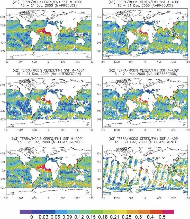
APRIL 2005 IGNATOV ET AL. 1011
tage of the strong absorption by water beyond 1 m (Li based upon analytical expressions, radiative transfer
et al. 2003). Pixels that pass all tests are sorted by re- calculations, empirical models, atmospheric correc-
flectance at 0.855 m, and the lower and upper 25% are tions, and interpolations. The difference or ratio be-
excluded. If the central 50% include at least 10 pixels tween the measured and expected values is compared
within the 20 ⫻ 20 window, the reflectances in each of with a threshold estimated as a function of sun-view
the seven MODIS bands 1–7 (from 0.466 to 2.119 m) geometry by trial and error, from comparisons of pre-
are averaged and checked if outside the glint area (␥ ⬎ dicted and observed clear values and from efforts to
40°) and internally consistent. minimize the view angle dependence of the retrieved
Aerosol lookup tables (LUTs) are applied to the av- cloud amount. The most critical tests for aerosol re-
erage reflectances in only six (1–2 and 4–7 on Terra) or trievals are the uniformity and adjacency tests. The uni-
five bands (1–2, 4–5, and 7 on Aqua) ranging from formity test is applied to sets of four clear pixels in a 2
⬃0.55 to 2.1 m. Band 3 (0.47 m) is not used because ⫻ 2 subsampled array mentioned at the start of section
of its response to materials like phytoplankton beneath 2. The difference between the maximum and minimum
the ocean surface. AOD for band 3 is modeled from the reflectance at 0.644 m must be less than 3 ⫻ 10⫺3
other bands. Retrieved AODs are reported in all seven (0.3%). The adjacency test further requires that all
bands 1–7 ranging from ⬃0.47 to 2.1 m. The aerosol eight pixels surrounding a candidate pixel are clear. In
size distribution is assumed to be a mix of two frac- addition to the ␥ ⬎ 40° threshold, the A-product glint
tions—fine and coarse—each being represented by a identification requires that all pixels on the solar side of
single lognormal mode. The algorithm chooses one fine the orbit are excluded. (This convention is currently
(out of four) and one coarse (out of five) mode and being reevaluated.) Reflectances in all cloud/glint-free
solves for their ratio and aerosol concentration. The
MODIS pixels within a CERES footprint are averaged
surface characteristics follow the isotropic Cox and
as explained in Geier et al. (2003).
Munk (1954b) model with a wind speed 6 m s⫺1. Aero-
AODs in bands 1 and 6 (7 for Aqua), A1 and A2, are
sol inversions are made with nine five-dimensional
estimated assuming that aerosol microphysics and all
LUTs, one for each aerosol mode: 15 view zenith
nonaerosol factors are fixed and invariant over global
angles, 15 sun zenith angles, 46 relative azimuth angles,
oceans (Ignatov et al. 2004). Single-channel Second
and 4 AODs in six bands. In the error minimization
procedure, linear mixtures of different pairs of fine and Simulation of the Satellite Signal in the Solar Spectrum
coarse modes are tested, with different weights. The (6S) radiative transfer model (RTM)-based (Vermote
LUTs have been precalculated using the Ahmad– et al. 1997) LUTs were constructed as described by
Fraser (1982) vector code at the six monochromatic Ignatov and Stowe (2002a) for the average MODIS
wavelengths, for the atmosphere containing molecules relative spectral response functions (see Fig. A1 in ap-
and aerosols and bounded by a rough ocean surface pendix A) and applied to the CERES-footprint average
from below. cloud-free reflectances, . The resulting retrieved are
reported at the centroid wavelengths of 1 ⫽ 0.63 and
b. A processing 2 ⫽ 1.61 m (2 ⫽ 2.119 m for Aqua). Note that the
Two elements of the A-product processing, data flow reference wavelengths in the A product slightly differ
and screening nonaerosol pixels, are detailed in Minnis from eff in the M product. For the comparisons in this
et al. (1999, 2004, unpublished manuscript) and Trepte study, A available on the CERES SSF datasets have
et al. (1999) (and summarized by Ignatov et al. 2005, been rescaled to the wavelengths at which the M are
unpublished manuscript). The other three elements— reported as follows: A1(0.644 m) ⫽ 0.96377 A1(0.630
aerosol algorithm, radiative transfer model, LUTs—are m) and A2(1.632 m) ⫽ 0.96716 A2(1.610 m).
identical to the third-generation AVHRR algorithm (Note that no scaling is needed for the A2 on Aqua.)
documented in (Ignatov and Stowe 2002a; Ignatov et al. The Ångström exponent is derived from rescaled as
2004). The A processing uses MODIS radiances, LEV, follows:
at the 1-km resolution (MOD02 1-km product, see ap-
pendix A for definitions), subsampled to every second 1
line/pixel, effectively reducing the data volume by a ␣ ⫽ ⌳ × ln共1Ⲑ2兲, ⌳ ⬅ ⫺ . 共1兲
factor of 4. To be used for aerosol retrievals a pixel ln共1Ⲑ2兲
must be over water, away from sun glint, cloud free, and
pass uniformity and adjacency aerosol tests. Cloud Note that the A-to-M conversion factors are close to
screening involves a sequence of three cascading unity (within ⬃3.5%) due to the proximity of eff used
threshold tests. The measured reflectance at 0.644 m in the A and M products. Their further refinement is
and brightness temperatures at 3.7, 11, and 12 m, and possible based on the estimated Ångström exponent,
different combinations thereof, are compared with but its effect on the accuracy of the scaling is negligible.
their expected values (Trepte et al. 1999). The expected The spectral amplification factor in Eq. (1), ⌳, is ⌳ ⬇
values are specified as functions of geographical loca- 1.08 for bands 1 and 6 (1⫽0.644, 2⫽1.632 m), and
tion, time, and illumination–observation geometry, ⌳ ⬇ 0.83 for bands 1 and 7 (1⫽0.644, 2⫽2.119 m).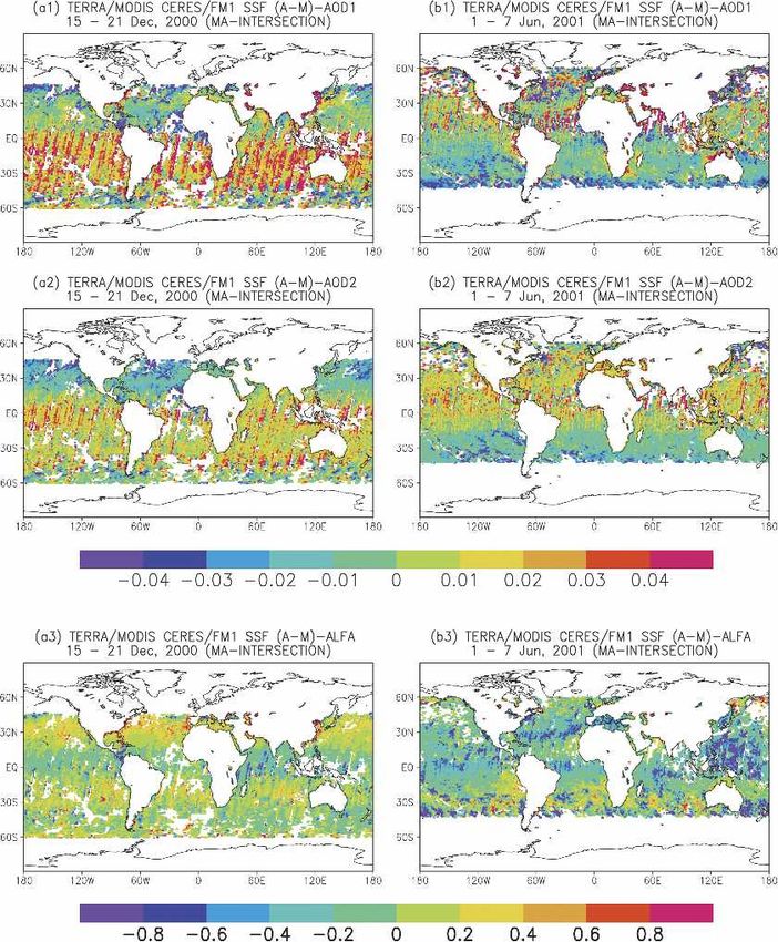
1012 JOURNAL OF THE ATMOSPHERIC SCIENCES—SPECIAL SECTION VOLUME 62
TABLE 2. Aerosol products on the Terra and Aqua CERES SSF datasets.
Ocean (M product) Ocean (A product) Land (M product)
Total count of MODIS pixels in a CERES
FOV, A–NT
% cloud fraction in a CERES FOV, % cloud fraction in a CERES FOV, A–FC (%) % cloud fraction in a CERES FOV
M–FC (%)
% of CERES FOV with aerosol, % of CERES FOV with aerosol, A–FA (%) % of CERES FOV with aerosol
M–FA (%)
M@466 nm @466 nm
M@553 nm @553 nm
M@644 nm A@630 nm @644 nm
M@865 nm A—Aerosol radiance @630 nm Mean reflectance @466 nm
M@1243 nm Mean reflectance @644 nm
M@1632 nm A@1610nm (Terra) Mean reflectance @865 nm
A—Aerosol radiance @1610 nm (Terra)
M@2119 nm A@2119nm (Aqua) Mean reflectance @2130 nm
A—Aerosol radiance @2119 nm (Aqua)
M-solution index (small fraction) Mean reflectance @3750 nm
M-solution index (large fraction) Std dev reflectance @466 nm
M@553 nm (small fraction) Aerosol types
M@865 nm (small fraction) Dust weighting factor
M@2119 nm (small fraction) Number of pixels (percentile)
M-cloud condensation nuclei (CCN)
c. M- and A-aerosol products on the CERES SSF 3. Preliminary evaluation of the M and A products
Table 2 lists all of the aerosol and related ancillary
on Terra CERES SSFs
parameters available on the Terra and Aqua CERES Differences between the M and A products on the
SSF datasets. The physical meaning of each is either CERES SSFs are expected because of 1) different sam-
self-explained, discussed below, or found in Kaufman et pling (cloud and glint screening); 2) different aerosol
al. (1997), Tanré et al. (1997), REM, and Geier et al. algorithms (including different treatment of aerosol mi-
(2003). Mapping specifics of the M- and A-aerosol crophysics, Rayleigh scattering, gaseous absorption,
products on the CERES SSF are summarized in appen- surface reflectance, radiative transfer model used to
dix B. generate the lookup tables, and numerical inversion
The aerosol radiances used to retrieve the MOD04 methods); and 3) different propagation of data errors
M over ocean were not saved, even though the M in all resulting from sensor calibration and other radiometric
seven MODIS bands are retained. (Note that the aero- uncertainties in the M and A products. In this section,
sol reflectances were saved in the land M product, the two products are compared and their observed dif-
which is not analyzed in this study.) In contrast, the A ferences are discussed in terms of the potential error
product reports A in only two bands and retains the sources, 1, 2, and 3.
aerosol radiances. Offline testing of a new aerosol al-
gorithm with the CERES SSF data is thus possible for
a. Defining the M and A (sub)samples: Statistics
the A product but not for the M product. In addition to
M, the M product over ocean includes other param-
for December 2000 and June 2001
eters that are listed in Table 2 but not used in this Statistics superimposed in Fig. 1 show that there are
analysis. In this study, three M and A counterparts are from ⬃2.2 to 2.3 million CERES footprints with at least
analyzed: A1 versus M1, A2 versus M2, and ␣A versus ␣M. one M- or A-aerosol retrieval in December 2000 and
Ancillary data listed in the first two lines of Table 2 from 2.5 to 2.6 million in June 2001. Hereafter, these
include cloud amount, FC (percent), and aerosol frac- datasets are referred to as the MA union samples, or
tion, FA (percent), in each CERES footprint. In addi- M 丣 A ⬅ A 丣 M, and are considered ⫽100%, by
tion, the A product provides a total count of MODIS definition. In a union sample, there are some CERES
pixels in a CERES FOV, NT (no M-product counter- FOVs in which both M- and A-product retrievals are
part is available for the A–NT parameter). In the pre- available. They form a subsample that is termed the
liminary analyses below, only the A-product param- MA intersection: M 嘸 A ⬅ A 嘸 M. Figure 1 shows
eters are used (cloud fraction, FC, and aerosol pixel that the MA intersection accounts for ⬃45% of the
count, NA ⫽ NT ⫻ FA /100%). The M-product param- union sample. In some CERES FOVs, only the M re-
eters will be explored in future work. trievals are available (but the A retrievals are not); this
APRIL 2005 IGNATOV ET AL. 1013
flect the M or A products (i.e., full M and A samples).
The similarity between the two patterns is quite impres-
sive, considering the large differences in the processing
procedures. Aerosol loading is elevated near some
landmasses (e.g., off Sahara, Saudi Arabia, India, and
Southeast Asia) and in some open ocean regions [e.g.,
intertropical convergence zone (ITCZ) and the stormy
“40°S” zonal belt]. It is unclear whether these latter
features are “real” or indicative of retrieval problems,
but in any case they are common to both products.
Although the A product has more missing data com-
pared to the M product, it extends farther south than
the M product, while the opposite is true in the North-
ern Hemisphere. These features are mainly a conse-
quence of excluding the solar side of the orbit in the A
FIG. 1. Count of CERES footprints with valid aerosol retrievals product.
in four datasets: December 2000 and June 2001, FM1 and FM2. In Figs. 2a(2) and 2b(2), based on MA intersection
The union sample, M丣A (defined as 100%) consists of all FOVs
in which either M- or A-aerosol retrievals are available. (Corre-
data, the differences between the 1M and 1A are
sponding counts of CERES FOVs are listed in the top of the mainly (yet not solely) due to the differences in the
figure.) The intersection sample, M嘸A (⬃45% of the union multichannel MOD04 and single-channel A-product al-
sample, on average), consists of all FOVs in which both M- and gorithms. The two products are highly correlated. For
A-aerosol retrievals are available. The M complement, M両A example, for FM1, the linear correlation coefficient, R,
(⬃45% of the union sample, on average) consists of all FOVs in
which the M retrievals are available but the A retrievals are not. equals 0.84 and 0.78 in December 2000 and June 2001,
The A complement, A両M (⬃10% of the union sample, on aver- respectively. The differences between the two datasets
age), consists of all FOVs in which the A retrievals are available are smaller than those for the full M and A products in
but the M retrievals are not. Figs. 2a(1)and 2b(1), implying that the effect of the
aerosol algorithm is less important than the effect of
sampling. Another interesting feature is that 1M in the
subset is called the M complement, or M両A. Likewise,
MA intersection is generally smaller than in its full
the footprints having only A retrievals (but not M re-
product counterpart, whereas 1A is comparable in both
trievals) form the A complement, or A両M. The M and
cases. This suggests that 1M is larger in the M comple-
A complements account for another ⬃45% and ⬃10%
ment than it is in the intersection sample.
of the union sample, respectively. The M and A
This is directly confirmed in Figs. 2a(3) and 2b(3)
complements highlight the effect of different sampling
produced from the M and A complements. The 1M in
procedures (glint screening and cloud clearing) on the
the M complement is clearly larger than the optical
retrievals, whereas the MA intersection can be used to
depths in both the MA intersection and the M product.
examine the effect of the aerosol algorithm differences.
The difference is less pronounced in the A comple-
The MA intersection and the M and A complements
ment, which consists of only ⬃10% of the union sample
divide the union sample into three nonoverlapping sub-
and, therefore, has many data gaps. [Note that, al-
samples from which other subsets can be constructed.
though the maps in Figs. 2a(3) and 2b(3) were pro-
In particular, the full M sample (referred to as the “M
duced from nonoverlapping CERES footprints, there
product”) comprises all footprints with valid M retriev-
may be overlap due to averaging of individual CERES
als, regardless of A product availability. It is thus de-
footprints within 7 day ⫻ (1°)2 grids.]
fined as a union of the MA intersection and the M
Figure 3 shows plots of the global distribution of 2.
complement: M ⬅ (M 嘸 A) 丣 (M 両 A) and accounts
The Saharan dust region, dominated by large particles,
for ⬃90% of the union sample. Likewise, the full A
is clearly evident, whereas smoke plumes with small
sample (the “A product”) is a union of the MA inter-
particles around India, Saudi Arabia, and Southeast
section and A complement, A ⬅ (M 嘸 A) 丣 (A 両 M)
Asia are not as prominent as in Fig. 2. The 2 results
and accounts for only ⬃55% of the union sample. The
have many points in common with the 1 results: 1)
large difference between the M and A samples mainly
differences between the three subsamples in the M
results from excluding the solar side of the orbit in the
product are significant, whereas the A product is more
A product processing.
uniform across all three subsamples, and 2) the M and
A products are most consistent in the MA intersection
b. M- and A-aerosol retrievals: Global distribution (for 2M and 2A, R ⫽ 0.61 and 0.68 in December 2000
in different samples and June 2001, respectively). In both products, orbital
Figure 2 plots the global distribution of 1 in Decem- striping seems to emerge more clearly in 2 compared
ber 2000 for the M and A products (columns) in the to the 1 image.
three subsamples (rows). Figures 2a(1) and 2b(1) re- The global distribution of the Ångström exponent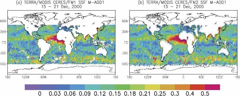
1014 JOURNAL OF THE ATMOSPHERIC SCIENCES—SPECIAL SECTION VOLUME 62
FIG. 2. (left) Mapping 1M (right)and 1A products for different subsamples (data of Terra CERES SSF FM1, Dec 2000): (a1), (b1)
full product [M ⬅ (M 嘸 A) 丣 (M 両 A), A ⬅ (M 両 A) 丣 (A 嘸 M)]; (a2), (b2) MA intersection (M 嘸 A); (a3), (b3) M and A
supplements [(M 両 A) and (A 両 M)].
(␣) from the M and A products is shown in Fig. 4. traced in both ␣M and ␣A retrievals. South of 60°S, ␣M
Observations 1 and 2 above for the maps also apply to retrievals are not available and ␣A data are clearly in
␣. The correlation between the ␣ fields in the MA in- error.
tersection is weaker compared to the fields (R ⫽ 0.57
c. M- and A-aerosol retrievals: Global statistics
and 0.38 in December 2000 and June 2001, respec-
tively). This is due to the high sensitivity of the aerosol Figure 5 summarizes the average statistics of the M
size parameter to errors, especially at low aerosol and A /␣ for December 2000 and June 2001 for FM1
loadings over ocean (Ignatov et al. 1998; Ignatov 2002; and FM2. For each dataset, we provide two A statistics,
Ignatov and Stowe 2002b). Orbital stripes are clearly based on panels b(2) and b(3) in Figs. 2–4, and two MAPRIL 2005 IGNATOV ET AL. 1015
FIG. 3. As in Fig. 2 but for 2.
statistics based on panels a(2) and a(3) in Figs. 2–4. tween the MA intersection and the A complement;
Statistics for the M and A products in a(1) and b(1) in clusters “1” and “2”) are generally smaller than the
Figs. 2–4 fall between their intersection and comple- sample-induced M differences. The only exception
ment counterparts and therefore are not shown here. is the ␣A statistics in cluster 1 for June 2001, where
The following observations emerge from Fig. 5: the A complement is very small and its statistics are
not globally representative (see analyses in section
(a) The M complement (cluster “4”) clearly stands out 3d and Fig. 6).
as different from the MA intersection (cluster “3”). (c) AOD is lower in June 2001 compared to December
The only difference between clusters 4 and 3 is sam- 2000. This difference is statistically significant in
pling, as the M-aerosol algorithm is the same here. both bands 1 and 6, in both SSF datasets (FM1 and
(b) Sampling-induced differences in the A product (be- FM2), and in both products (M and A).1016 JOURNAL OF THE ATMOSPHERIC SCIENCES—SPECIAL SECTION VOLUME 62
FIG. 4. As in Fig. 2 but for ␣.
(d) Aerosol algorithm-induced global differences be- d. Possible causes for the sampling M differences
tween the M and A retrievals in the MA intersec-
tion (cluster 2 versus 3) are within ⬃(4 ⫾ 5) ⫻ 10⫺3 To help determine if the M sampling differences be-
for 1; within ⬃(3 ⫾ 1) ⫻ 10⫺3 for 2, and within tween clusters 3 and 4 are due to geographical differ-
⬃(1 ⫾ 1) ⫻ 10⫺1 for ␣. ences, Fig. 6 shows the average latitude and longitude
(e) The FM2 statistics are somewhat higher com- statistics for the four datasets (note that the statistics
pared to their FM1 counterparts. The cause for this are identical for clusters 2 and 3, which represent dif-
difference is not entirely clear, but is likely related ferent aerosol retrievals in the same MA intersection
to sampling as opposed to aerosol algorithm differ- domain). The latitude–longitude statistics of the M
ences. complement (cluster 4) and MA intersection (cluster 3)APRIL 2005 IGNATOV ET AL. 1017
cinity of the aerosol retrievals, and five angles. Again,
all statistics in clusters 2 and 3 are identical. Three clus-
ters, 1–3, form a more or less uniform group, whereas
the M supplement (cluster 4) clearly stands out in the
average cloud amount, relative azimuth, and scattering
angle histograms.
1) Cloud amount is AT ⬃39% in clusters 1–3, whereas
it is 59% in cluster 4. It should be noted that the AT
is a conditional estimate (i.e., only those CERES
footprints were used with at least one aerosol re-
trieval), and that cloud amounts used here come
from the A product.
2) Relative azimuth angle is ⬃125° in clusters 1–3 com-
pared to ⬃86° in cluster 4. The relative azimuth can-
not be less than 90° in the A retrievals, which are not
produced on the solar side of the orbit, but it may be
less than 90° in the M retrievals.
3) Scattering angle is ⬃142° in clusters 1–3 versus
⬃120° in cluster 4.
Understanding the mechanisms of how factors 1–3
may affect the aerosol retrievals is the subject of future
research (note also that some factors may be interde-
pendent or cross correlated, e.g., the relative azimuth
and scattering angles).
e. Possible causes for the December 2000–June
2001 aerosol differences
Figure 8 provides M versus A and ␣M versus ␣A for
June 2001, in the MA intersection. These are compared
with the corresponding December 2000 results in Figs.
2–4. The AODs in June 2001 are lower than in Decem-
ber 2000 in both bands. The difference is most promi-
nent in the cleanest remote areas of the Southern
Hemisphere and over the central Indian and Pacific
Oceans. Figure 8 confirms that the global aerosol sta-
tistics change significantly over the 51⁄2-month period.
This change is observed in both aerosol products and
far exceeds the differences between the M and A prod-
ucts in any given month. For instance, the average 1 is
⬃0.11 in December 2000 compared to 1 ⬃0.09 in June
2001. A similar change is observed in 2. Figures 6 and
7 suggest that these differences are not likely to be
related to differences in geography, cloud amount, or
viewing geometry. Figure 5 also shows that the Ång-
FIG. 5. Average statistics of aerosol retrievals in Dec 2000 and ström exponents change in a more complicated way
Jun 2001, FM1 and FM2 datasets. (Samples are defined in caption from December 2000 to June 2001. In the MA inter-
to Fig. 1.) section, ␣M increases from ⬃0.6 to ⬃0.7, whereas ␣A
decreases from ⬃0.6 to ⬃0.5. This is consistent with the
are very close, so geographical differences likely are not comparisons in Figs. 8 and 4a(2), b(2).
the reason for the observed differences. On the other The sensor radiometric performance is one possible
hand, the A complement (cluster 1) is displaced from cause for the observed aerosol changes. The MODIS
cluster 2 (especially in June 2001), which may explain underwent a number of changes and experienced some
the ␣A anomaly in the A complement in June 2001 in short interruptions due to instrument problems early in
Fig. 5. Terra operations after science data collection began 24
Figure 7 shows histograms of the six other factors February 2000. The MODIS A-side electronics (“A-I”)
associated with the retrievals: cloud amount in the vi- was used from 24 February to 26 October 2000. On 301018 JOURNAL OF THE ATMOSPHERIC SCIENCES—SPECIAL SECTION VOLUME 62
FIG. 6. Average latitude and longitude in Dec 2000 and Jun 2001, FM1 and FM2 datasets. (Samples defined in
caption to Fig. 1.)
FIG. 7. As in Fig. 6 but for (a1) ambient cloud amount; (b1) relative azimuth angle; (a2) solar zenith angle; (b2)
view zenith angle; (a3) scattering angle; and (b3) glint angle.APRIL 2005 IGNATOV ET AL. 1019 FIG. 8. Distribution in MA intersection of [a(1), b(1)] 1, [a(2), b(2)] 2, and [a(3), b(3)] ␣ derived from Terra CERES/FM1 SSF in Jun 2001: (left) M product and (right) A product. Compare with distributions in the MA intersection in Dec 2000: 1 in Figs. 2a(2)–b(2); 2 in Figs. 3a(2)–b(2); and ␣ in Figs. 4a(2)–b(2). (See discussion in section 3e.) October 2000, the B-side electronics (“B”) was enabled has performed as expected after the last switch (see and used until 15 June 2001. After experiencing a appendix A for definitions and more detail). power supply 2 (PS-2) shutdown anomaly, the MODIS The two datasets analyzed in this study, in December used the power supply 1 (PS-1) and the A-side elec- 2000 and June 2001, both belong to the same B elec- tronics (“A-II”). According to the MODIS Character- tronics/PS-2 period of MODIS life cycle, during which ization Support Team (MCST), the MODIS instrument the measurement quality improved dramatically ac-
1020 JOURNAL OF THE ATMOSPHERIC SCIENCES—SPECIAL SECTION VOLUME 62
cording to the MCST. However it is possible that some g. Cloud amount trends in aerosol retrievals
subtle radiometric changes continued to occur during
The cloud–aerosol correlations in the M and A prod-
this “stable” period, especially shortly before and after
ucts are examined to explore the possibility that the
the switches. Aerosol is known to be a very sensitive
aerosol sampling biases found in section 3d are caused
indicator of sensor radiometric uncertainties (Ignatov by cloud contamination. The top panels of Fig. 10 show
2002, 2003; Ignatov and Stowe 2002b; Ignatov et al. histograms of AT for December 2000 and June 2001. In
2004), but the M and A products may respond to cali- both products, the cloud amount is more or less uni-
bration errors differently. The M product weighs all formly distributed in the ⬃0%–80% range. Intuitively,
bands together in a complicated way. Its sensitivity to a progressively smaller proportion of aerosol observa-
(random in bands) calibration errors has been docu- tions is expected at high ambient cloud cover. This is
mented by Tanré et al. (1997), but the instrument indeed the case in the A product (at AT ⬎ 80%),
switches may not be random from band to band as they whereas the increasing trend in the M product is unex-
affect all bands coherently. For example, it has been pected.
observed that each switch affected the aerosol size pa- Figures 10a(2)–a(4) and 10b(2)–b(4) show aerosol re-
rameter estimated from MODIS (REM). On the other trievals as a function of AT. The trends in /␣ with AT
hand, the single-channel A algorithm emphasizes the are strong in both the M and A products. Similar trends
information content of each individual band. Thus the have been previously observed in the NOAA/AVHRR
opposite trends in the M and A Ångström exponents and TRMM/VIRS aerosol retrievals (Ignatov and Nalli
may be related to a different reaction of the M- or 2002; Ignatov et al. 2005, unpublished manuscript). The
A-product algorithms to radiometric perturbations in AT differences between the MA intersection (AT ⬃
different MODIS bands. More analyses are needed to 39%) and the M supplement [AT ⬃ 59%; cf. Fig. 7a(1)]
understand the observed change of aerosol parameters combined with the results in Fig. 10 suggest that cloud-
with time. screening differences between the M and A products
are the likely cause for the -retrieval differences ob-
served in Fig. 5. The aerosol–cloud correlations are ei-
f. Differences due to aerosol algorithm: Focus on ther “real” (increased hygroscopic aerosol particles that
the MA intersection influence cloud formation) or artifacts of the retrievals
Examination of the effect of M-aerosol and A- (residual cloud in a MODIS field of view). The in-
aerosol algorithm differences is best achieved by using creased sensitivity in M to AT, as compared to sensi-
the MA intersection where the effect of sampling is tivity of A to AT, suggests that the residual cloud is
minimized though not removed completely, as different definitely present and contributes to the observed
MODIS pixels within a CERES FOV could have been trends. However the Ångström exponent trends in Figs.
used by each algorithm. The respective A ⫺ M differ- 10a(4) and 10b(4) are consistent with both hypotheses:
ences are mapped in Fig. 9. The differences, which ␣⬃1 when AT ⬃ 0%, decreases to ␣ ⬃ 0.5 at AT ⬃
reach a few hundredths of , appear to increase with 20%–40%, and flattens thereafter. (Note that the ␣A
solar zenith angle and vary with scan position. More shows some residual artifacts at large AT that are not
analyses are needed to determine if the M, A, or both fully understood.) Further studies are needed to ex-
products are responsible for the patterns. These arti- plain these features.
facts may also be related to the aforementioned re- Figure 10 also reveals significant differences between
sidual sampling differences. For example, Guzzi et al. December 2000 and June 2001. In band 1, the minimum
(1998) indicate that residual cloud in a sensor FOV may in A is ⬃⫺0.04 in December 2000 and decreases to
cause artificial sun-angle trends in the retrieved AOD. ⬃⫺0.07 in June 2001. Negative values of are possible
in the A product, whereas the M product truncates
In December 2000 (Fig. 9, left), the biases in appear
negative retrievals. The seasonal shift in the A mini-
to be quasi multiplicative in both bands, suggesting that
mum is consistent with the shift in the mean values of
they mainly originate from differences between the M-
A in Fig. 5. If this difference was caused by a calibra-
and A-aerosol models (e.g., Ignatov and Stowe 2002a)
tion slope change, it would be equivalent to an ⬃3%–
and largely cancel out when their ratio is used to cal-
4% degradation over 5 months of Terra operation (Ig-
culate the Ångström exponent. In June 2001, the A ⫺
natov 2002). Change in calibration intercept may also
M differences are smaller, but there is no cancellation
contribute to the observed decline in (). In band 6, the
in calculating ␣, indicating the presence of additive er-
minimum 2A is slightly negative but close to zero due
rors in either A or M, or both. According to Ignatov
to truncation of negative radiances (see appendix A
(2002), additive errors may be caused by calibration
and Fig. A2).
slope uncertainties. As a result, the (␣A ⫺ ␣M) differ-
ences in June 2001 show large spatial variability, with
an overall negative bias of ⬃⫺0.2. The global ␣ statis- 4. Discussion and conclusions
tics in Fig. 5 are in quantitative agreement with this Two aerosol products over oceans available on the
visual estimate from Fig. 9. Terra and Aqua CERES SSF datasets reveal commonAPRIL 2005 IGNATOV ET AL. 1021
FIG. 9. Distribution in MA intersection of [a(1), b(1)] 1A–1M; [a(2), b(2)] 2A–2M; and [a(3), b(3)] ␣A–␣M derived from Terra
CERES/FM1 SSF in (left) Dec 2000 and (right) Jun 2001. (See discussion in section 3f.)
features and some differences due to different sampling (such as the ocean surface reflectance, Rayleigh scat-
and aerosol algorithms. tering, gaseous absorption, RTM, and numerical inver-
The M- and A-product aerosol algorithms differ sig- sion) that are treated differently. Their cumulative re-
nificantly. The globally invariant aerosol model in the sult can be assessed only through empirical analyses.
A product is clearly a limitation, which is purportedly The MA intersection sample constructed in this study is
alleviated in the M product. Note also that there are best suited to highlight the aerosol algorithm differ-
many nonaerosol factors in the aerosol algorithms ences. The comparisons demonstrate that aerosol algo-1022 JOURNAL OF THE ATMOSPHERIC SCIENCES—SPECIAL SECTION VOLUME 62
FIG. 10. [a(1), b(1)] Histograms of cloud amount, AT (⌬AT ⫽ 5%), and [a(2)–b(4)] aerosol retrieval trends for
(left) Dec 2000 and (right) Jun 2001 datasets. (See discussion in section 3g).APRIL 2005 IGNATOV ET AL. 1023 rithm-induced global differences between the M and A channel A products differently. This example highlights retrievals are within ⬃(4 ⫾ 5) ⫻ 10⫺3 for 1, ⬃(3 ⫾ 1) the need for a continuous in-flight monitoring of the ⫻ 10⫺3 for 2, and ⬃(1 ⫾ 1) ⫻ 10⫺1 for ␣. The M ⫺ A performance of all individual bands of both MODIS differences appear to be sun angle and scan position instruments. This should be done as a part of an aerosol dependent, and may reach ⫹0.04 in certain domains of quality assurance process as an addition to the MODIS sun-view geometries. Some residual sampling discrep- Characterization Support Team tests. ancies may still contribute to the observed differences. Aerosol retrievals are obtained from the lowest ob- The aerosol algorithm differences are currently being served radiances and thus are very sensitive to even the analyzed in depth, and the results will be reported else- smallest radiometric uncertainties and residual errors where. of cloud and glint screening. Including single-channel However, most of the discrepancy between the two A-type retrievals from each MODIS band used in the products is due to different sampling. The M products standard MOD04 processing would provide an excel- are available in ⬃90% of the union MA sample, lent indicator of overall band performance from an whereas the A products occur in only ⬃55%. Aerosol aerosol user perspective. Such work should also be statistics in the M supplement (M product only) differs closely coordinated with the ocean color retrievals, from the MA intersection sample by ⬃⫹(0.030 ⫾ which are known to be even more demanding to the 0.003) for both 1 and 2, and by ⬃⫺(0.20 ⫾ 0.05) for ␣. input data accuracy (G. Feldman and C. McClain 2004, The A-product differences between the A supplement personal communication). We also recommend an end and MA intersection are statistically insignificant. A to the current double truncation of negative radiances possible explanation is related to the fact that aerosol on the level 1B processing and negative aerosol optical retrievals strongly correlate with the ambient cloud depths in the MOD04 processing. Regular (at least one amount in both products, although the dependence on orbit per day) collection of data in the solar reflectance cloud amount in the M product is more pronounced bands on the dark side of the earth would help to moni- than in the A product. Similar cloud–aerosol correla- tor the radiometric performance of the solar reflectance tions have been observed previously in the NOAA/ bands (Ignatov 2003). These steps could improve the AVHRR and TRMM/VIRS aerosol retrievals. Draw- ability to monitor/diagnose the actual performance of ing a line between the cloud and aerosol is ambiguous. the MODIS instrument in-flight and greatly facilitate Selecting the thresholds in the cloud screening algo- correcting any problems. As an improvement to the rithms is not a completely objective procedure. Note current CERES SSF processing, saving six MODIS ra- that Myhre et al. (2004) compared five different aerosol diances used for the MOD04 retrievals over oceans products derived from four satellite sensors on three (which are available on MOD04 product) on the SSF platforms and concluded that the major cause for the datasets would greatly benefit their utility for aerosol observed aerosol differences are likely due to the dif- analyses and improvements. ferences in cloud screening. Further study is needed to The exact comparison numbers may be refined in the resolve these issues. Other reasons for differences be- future, as newer collections of MOD04 products (004 tween the two aerosol products are likely related to a and 005) become available, and the A processing un- different domain of scattering and/or relative azimuth dergoes some changes (such as, i.e., change in sampling geometries for the samples remaining after cloud and from every second line/second pixel to every second glint screening. line/fourth pixel). Nevertheless, these initial compari- Comparison of the global December 2000 and June sons of the two MODIS-based marine aerosol products 2001 statistics indicate a systematic decrease in aerosol indicate that the more spectrally complex MOD04 and optical depths over the 51⁄2- month period in both prod- simpler AVHRR-type aerosol methods produce rela- ucts. The two-band analyzed in this study (0.644 and tively consistent results. Although further detailed 1.632 m) change in the same direction but not exactly analyses of the datasets used here and later retrievals coherently, leading to opposite trends in the Ångström will provide information necessary to fully reconcile the exponents in the two products: the ␣M increases by discrepancies, it appears that a reliable linkage can be ⬃ ⫹0.1 whereas the ␣A decreases by ⬃ ⫺0.1. Neither of established between the older record based on the sim- these changes is associated with a significant shift in the pler methods and the current and future retrievals using geographic or angle domain or in the cloud amount. more sophisticated approaches. With that connection, it Seasonal change, if extant, would be minimal in the will be possible to establish a trustworthy and valuable most pristine ocean areas and therefore is unlikely to long-term climatology of oceanic aerosol properties. affect the minimum in . However, the band-1 A prod- uct clearly shows a decline of ⬃ 0.03 in the minimum Acknowledgments. The MOD04 algorithms were de- from December 2000 to June 2001. An analysis of veloped in late 1990s by the international team of sci- band-6 minima is impossible due to radiance trunca- entists (NASA GSFC, United States, and Laboratoire tion. A possible explanation for the change in the d’Optique Atmospherique, University of Lille, France) minima is the variation in the MODIS performance, under energetic and enthusiastic leadership of Yoram which affects the multichannel M and the single- Kaufman. The A-product retrievals were initiated in
1024 JOURNAL OF THE ATMOSPHERIC SCIENCES—SPECIAL SECTION VOLUME 62
late 1980s by Nagaraja Rao (deceased) and Larry tation. The views, opinions, and findings contained in
Stowe (retired) at NOAA/NESDIS following the pio- this report are those of the authors and should not be
neering ideas by Michael Griggs proposed in mid- construed as an official NOAA or U.S. Government
1970s. The A product has been enhanced and applied position, policy, or decision.
to other sensor data (TRMM VIRS, and Terra/Aqua
MODIS) under the CERES project. The authors are APPENDIX A
indebted to Jack Xiong, Bill Barnes, Bruce Guenther
(NASA GSFC-MCST), Chris Moeller (University of MODIS Definitions
Wisconsin—Madison), Kurt Thome (The University
of Arizona), and Chagyong Cao and Jerry Sullivan MODIS takes measurements in 36 spectral bands, of
(NOAA/NESDIS) for helpful discussions of the which 20 are solar reflectance bands (SRBs: see MCST
MODIS radiometric issues. Help and advice from Rich- 2002a,b; Xiong et al. 2002; and http://www.mcst.ssai.biz/
ard Hucek, Shana Mattoo, Allen Chu, Rob Levy, mcstweb/index.html). MODIS level 1B data (termed
Rong-Rong Li, Vincent Chiang, and Gwyn Fireman MOD02 and MYD02 for Terra and Aqua, respectively)
(NASA GSFC), and Qing Trepte and Robert Arduini are available in three spatial resolutions: 250 m in bands
(NASA LaRC) is also appreciated. This work was 1–2 [Q(uarter) km]; 500 m in bands 1–7 [H(alf) km; in
funded under the NASA EOS/CERES (NASA Con- bands 1–2, 2 ⫻ 2 pixels are aggregated]; and 1000 m in
tract L-90987C), the Integrated Program Office (IPO/ all bands [1 km; in bands 1–2 and 3–7, 4 ⫻ 4 and 2 ⫻ 2
NOAA/NASA/DOD), NOAA Ocean Remote Sens- pixel averaging is done].
ing, and Joint Center for Satellite Data Assimilation Each band is characterized by a finite relative spec-
(NOAA/NESDIS) Programs. We thank Steve Mango tral response (RSR; Fig. A1). Higher spatial resolution
(IPO) and Bill Pichel and Fuzhong Weng (NOAA/ in aerosol bands (250/500 m in bands 1–2/3–7; 1000 m in
NESDIS) for their support and encouragement. The all other bands) is achieved through the use of 40/20
Terra CERES SSF data used in this study were ob- detectors per band, respectively. All RSRs are sup-
tained from the Atmospheric Sciences Data Center at posed to be the same for all detectors within a band and
NASA Langley Research Center. Thoughtful and con- for similar bands of the two instruments but, in fact,
structive reviews by Tom Charlock and Bill Smith Jr. they slightly vary, as shown in Fig. A1. The “effective”
(NASA LaRC), and by two anonymous reviewers were wavelength, eff, is customarily used to identify a band’s
instrumental for improved style and clarity of presen- spectral position. The definition of eff may be not
FIG. A1. RSR of the MODIS bands used in the AVHRR-like retrievals (a) 1 and (b) 6(7) on (top)
Terra and (bottom) Aqua. Superimposed are reference wavelengths at which the A and M products are
reported. (Solid lines represent average RSRs over the 40/20 detectors, and shaded areas show cross-
detector variability.)APRIL 2005 IGNATOV ET AL. 1025
TABLE A1. Effective central wavelengths eff (nm) for seven MODIS bands used in M-aerosol retrievals over ocean. Values of eff
(bands 1–3) cited in literature and (bands 4–5) calculated in this study according to Ignatov and Stowe (2002a) for MODIS PFM (Terra)
and FM1 (Aqua) filters (available online at http://www.mcst.ssai.biz/mcstweb/info/faq.html). Values by REM are used throughout this
work.
Reference
Current work
Band (No. of 1) Xiong et al. 2) Tanré et al.
detectors) (2002) (1997) 3) REM 4) Terra Mean (std dev) 5) Aqua Mean (std dev)
1 (N ⫽ 40) 645 659 644 645.8 (0.011) 645.3 (0.002)
2 (N ⫽ 40) 858 865 855 856.2 (0.012) 856.6 (0.009)
3* (N ⫽ 20) 469* 470* 466* 465.7* (0.007) 466.0* (0.002)
4 (N ⫽ 20) 555 555 553 553.7 (0.004) 553.9 (0.002)
5 (N ⫽ 20) 1240 1240 1243 1242.0 (0.032) 1241.3 (0.014)
6 (N ⫽ 20) 1640 1640 1632 1629.1 (0.030) 1627.9 (0.012)
7 (N ⫽ 20) 2130 2130 2119 2113.6 (0.019) 2113.4 (0.011)
* Band 3 on both platforms and band 6 on Aqua are not used. They are listed for reference only.
unique. Shown in Table A1 are different values of eff able from L1B files. Columns 1 and 3 of Table A2 list,
cited in MODIS literature (columns 1–3) and our own by band, the mean and standard deviation of the indi-
calculations of eff performed for this study (columns vidual-detector Feff as read directly from the L1B data.
4–5). The latter two columns report mean and standard Note that the LEV product on L1B is estimated from
deviation (std dev) statistics, over all 40/20 detectors, of the EV o using the mean Feff (MCST 2002b). For
eff calculated by applying equations from Ignatov and comparison, columns 2 and 4 of Table A2 list the mean/
Stowe (2002a) to the RSR of each individual detector. standard deviation statistics of our own calculations of
The small standard deviations indicate overall excellent Feff following Ignatov and Stowe (2002a). In bands 1, 2,
reproducibility of the RSRs within a band: std dev (eff) and 4 (from ⬃0.55 to 0.85 m), the two Feff agree within
ⱕ 0.03 nm for Terra, and ⱕ 0.01 nm for Aqua. In this a few tenths of a percent. For shorter (band 3) and
study, the eff listed in column 3 after REM are used for longer (bands 5–7) wavelengths, the differences reach a
consistency with the MODIS aerosol group who report few percent, possibly due to the uncertainties in the
their retrievals at these eff. solar spectrum for narrow spectral intervals. These dif-
MODIS L1B SRB data contain two standard prod- ferences hint at possible errors and need further clari-
ucts: the (earth-view overhead) reflectance, EV o fication. The MCST (2002) values are used in this study,
(o ⬅ coso, o is the solar zenith angle), and the (earth- for consistency with the mainstream GSFC processing.
view) radiance, LEV (MCST 2000, 2002a,b; Xiong et al. For reference, Table A3 summarizes our calculations of
2002). Reflectance normalized at earth–sun (ES) dis- Rayleigh, R, and gaseous, G, optical depths in the
tance of dES ⫽ 1 AU is the primary product, from which seven MODIS SRBs for the six standard atmospheres.
the spectral radiance, LEV,i (W m⫺2 m⫺1 sr⫺1) (not These data are referred to and discussed in the text.
normalized at dES ⫽ 1 AU) is derived as Feff,i EV,i Aerosol retrievals over ocean rely on the lowest
2
0/dES . Here, Feff,i (W m⫺2 m⫺1 sr⫺1) is the solar spec- TOA radiances, which are very challenging to measure
tral irradiance normalized with and at dES ⫽ 1 AU. accurately due to larger relative contributions from ra-
The values of Feff for all bands and detectors are avail- diometric noise, digitization, and possible calibration
TABLE A2. Mean (std dev) statistics (over N detectors) of effective “solar constants,” Feff (W m⫺2 sr⫺1 m⫺1), for the seven bands
used in aerosol retrievals over ocean for MODIS (bands 1–2) PFM (Terra) and (bands 3–4) FM1 (Aqua). Data: (bands 1,3) derived from
the “Solar Irradiance on RSB Detectors over pi” global attribute on MODIS L1B (MCST 2002b); (bands 2,4) calculated in current
study according to Ignatov and Stowe (2002a). [Percent deviation from MCST (2002b) is also shown.] Values of Feff listed on MODIS
L1B (bands 1,3) are used throughout this work.
MODIS PFM (Terra) MODIS FM1 (Aqua)
Band / eff (No. of detectors) 1) MCST(2002b) 2) Current study 3) MCST (2002b) 4) Current study
1 / 644 nm (N ⫽40) 511.26 (0.607) 510.19/⫺0.21% (0.039) 511.86 (0.185) 510.74/⫺0.22% (0.008)
2 / 855 nm (N ⫽40) 315.83 (0.142) 316.20/⫹0.12% (0.040) 315.55 (0.118) 315.96/⫹0.13% (0.037)
3* / 466 nm (N ⫽20) 664.61* (0.032) 641.57/⫺3.47% (0.018) 664.69* (0.071) 641.57/⫺3.48% (0.046)
4 / 553 nm (N ⫽20) 593.95 (0.024) 592.22/⫺0.29% (0.005) 593.74 (0.050) 592.16/⫺0.27% (0.017)
5 / 1243 nm (N⫽20) 150.99 (0.016) 145.59/⫺3.58% (0.015) 151.18 (0.006) 145.92/⫺3.48% (0.006)
6 / 1632 nm (N⫽20) 76.47 (0.015) 75.49/⫺1.28% (0.005) 76.59 (0.013) 75.67/⫺1.20% (0.001)
7 / 2119 nm (N⫽20) 28.75 (0.014) 30.29/⫹5.36% (0.001) 28.77 (0.003) 30.30/⫾5.32% (0.001)You can also read