Unveiling phase transitions with machine learning
←
→
Page content transcription
If your browser does not render page correctly, please read the page content below

Unveiling phase transitions with machine learning

                                                  Askery Canabarro,1, 2 Felipe Fernandes Fanchini,3 André Luiz Malvezzi,3 Rodrigo Pereira,1, 4 and Rafael Chaves1, 5
                                                                1 International Institute of Physics, Federal University of Rio Grande do Norte, 59078-970 Natal, Brazil
                                                                             2 Grupo  de Física da Matéria Condensada, Núcleo de Ciências Exatas - NCEx,
                                                                         Campus Arapiraca, Universidade Federal de Alagoas, 57309-005 Arapiraca-AL, Brazil
                                                                          3 Faculdade de Ciências, Universidade Estadual Paulista, 17033-360 Bauru-SP, Brazil
                                                          4 Departamento de Física Teórica e Experimental, Federal University of Rio Grande do Norte, 59078-970 Natal, Brazil
                                                                5 School of Science and Technology, Federal University of Rio Grande do Norte, 59078-970 Natal, Brazil

                                                                                                          (Dated: April 3, 2019)
                                                                  The classification of phase transitions is a central and challenging task in condensed matter
                                                               physics. Typically, it relies on the identification of order parameters and the analysis of singu-
                                                               larities in the free energy and its derivatives. Here, we propose an alternative framework to identify
                                                               quantum phase transitions, employing both unsupervised and supervised machine learning tech-
                                                               niques. Using the axial next-nearest neighbor Ising (ANNNI) model as a benchmark, we show how
                                                               unsupervised learning can detect three phases (ferromagnetic, paramagnetic, and a cluster of the
arXiv:1904.01486v1 [cond-mat.str-el] 2 Apr 2019

                                                               antiphase with the floating phase) as well as two distinct regions within the paramagnetic phase.
                                                               Employing supervised learning we show that transfer learning becomes possible: a machine trained
                                                               only with nearest-neighbour interactions can learn to identify a new type of phase occurring when
                                                               next-nearest-neighbour interactions are introduced. All our results rely on few and low dimen-
                                                               sional input data (up to twelve lattice sites), thus providing a computational friendly and general
                                                               framework for the study of phase transitions in many-body systems.

                                                                    I.   INTRODUCTION                                [31–35]. For instance, neural networks can detect local
                                                                                                                     and global order parameters directly from the raw state
                                                                                                                     configurations [31]. They can also be used to perform
                                                     Machine learning (ML) means, essentially, computer              transfer learning, for example, to detect transition tem-
                                                  programs that improve their performance automatically              peratures of a Hubbard model away from half-filling
                                                  with increasing exposition to data. The algorithmic im-            even though the machine is only trained at half-filling
                                                  provements over the years combined with faster and                 (average density of the lattice sites occupation) [33].
                                                  more powerful hardware [1–12] allows now the possi-                   In this paper our aim is to unveil the phase transi-
                                                  bility of extracting useful information out of the mon-            tions through machine learning, for the first time, in
                                                  umental and ever-expanding amount of data. It is the               the axial next-nearest neighbor Ising (ANNNI) model
                                                  fastest-growing and most active field in a variety of re-          [36, 37]. Its relevance stems from the fact that it is the
                                                  search areas, ranging from computer science and statis-            simplest model that combines the effects of quantum
                                                  tics, to physics, chemistry, biology, medicine and social          fluctuations (induced by the transverse field) and com-
                                                  sciences [13]. In physics, the applications are abundant,          peting, frustrated exchange interactions (the interaction
                                                  including gravitational waves and cosmology [14–24],               is ferromagnetic for nearest neighbors, but antiferro-
                                                  quantum information [25–27] and in condensed matter                magnetic for next-nearest neighbors). This combination
                                                  physics [28–30] most prominently in the characteriza-              leads to a rich ground state phase diagram which has
                                                  tion of different phases of matter and their transitions           been investigated by various analytical and numerical
                                                  [31–35].                                                           approaches [38–43]. The ANNNI model finds applica-
                                                     Classifying phase transitions is a central topic in             tion, for instance, in explaining the magnetic order in
                                                  many-body physics and yet a very much open problem,                some quasi-one-dimensional spin ladder materials [44].
                                                  specially in the quantum case due the curse of dimen-              Moreover, it has recently been used to study dynamical
                                                  sionality of exponentially growing size of the Hilbert             phase transitions [45] as well as the effects of interac-
                                                  space of quantum systems. In some cases, phase tran-               tions between Majorana edge modes in arrays of Kitaev
                                                  sitions are clearly visible if the relevant local order pa-        chains [46, 47].
                                                  rameters are known and one looks for non-analyticities                Using the ANNNI model as a benchmark, we pro-
                                                  (discontinuities or singularities) in the order parameters         pose a machine learning framework employing unsu-
                                                  or in their derivatives. More generally, however, uncon-           pervised, supervised and transfer learning approaches.
                                                  ventional transitions such as infinite order (e.g., Koster-        In all cases, the input data to the machine is con-
                                                  litz–Thouless) transitions, are much harder to be identi-          siderably small and simple, the raw pairwise correla-
                                                  fied. Typically, they appear at considerably large lattice         tion functions between the spins for lattices up to 12
                                                  sizes, a demanding computational task which machine                sites. First, we show how unsupervised learning can
                                                  learning has been proven to provide a novel approach               detect, with great accuracy, the three main phases of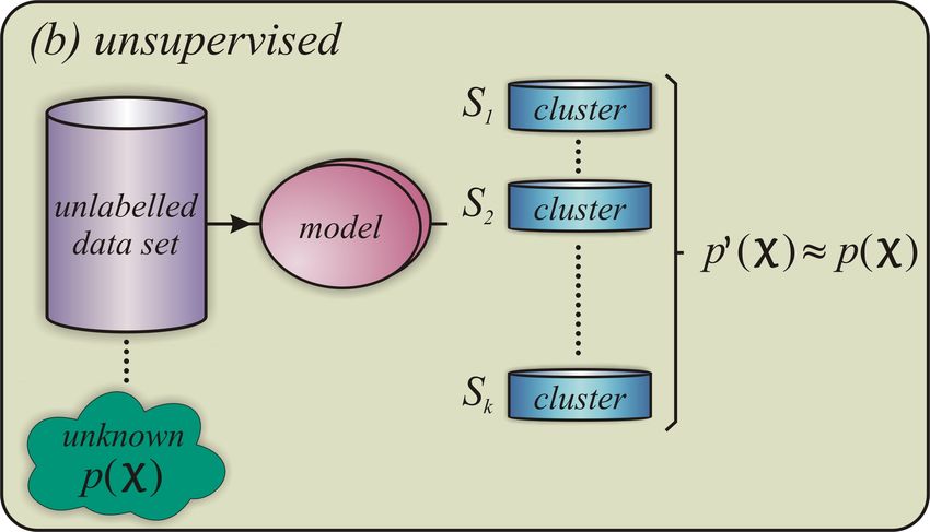
2

the ANNNI model: ferromagnetic, paramagnetic and                     ground states represented schematically by ↑↑↑↑↑↑↑↑,
the clustered antiphase/floating phase. As we show,                  the antiphase breaks the lattice translational symmetry
the unsupervised approach also identifies, at least qual-            and has long-range order with a four-site periodicity in
itatively, two regions within the paramagnetic phase as-             the form ↑↑↓↓↑↑↓↓. On the other hand, the paramag-
sociated with commensurate and in-commensurate ar-                   netic phase is disordered and has a unique ground state
eas separated by the Peschel-Emery line [48], a subtle               that can be pictured as spins pointing predominantly
change in the correlation functions which is hard to                 along the direction of the field. Inside the three phases
discern by conventional methods using only data from                 described so far, the energy gap is finite and all corre-
small chains (as we do here). Finally, we show how                   lation functions decay exponentially. By contrast, the
transfer learning becomes possible: by training the ma-              floating phase is a critical (gapless) phase with quasi-
chine with nearest-neighbour interactions only, we can               long-range order, i.e., power-law decay of correlation
also accurately predict the phase transitions happen-                functions at large distances. This phase is described by
ing at regions including next-nearest-neighbour inter-               a conformal field theory with central charge c = 1 (a
actions.                                                             Luttinger liquid [49] with an emergent U(1) symmetry).
   The paper is organized as follows. In Sec. II we                     The quantum phase transitions in the ANNNI model
describe in details the ANNNI model. In Sec. III we                  are well understood. For κ = 0, the model is integrable
provide a succinct but comprehensive overview of the                 since it reduces to the transverse field Ising model [50].
main machine learning concepts and tools we employ                   The latter is exactly solvable by mapping to noninter-
in this work (with more technical details presented in               acting spinless fermions. Along the κ = 0 line of the
the Appendix). In Sec. IV we present our results: in                 phase diagram, a second-order phase transition in the
Sec. IV A we explain the data set given as input to the              Ising universality class occurs at g = 1. It separates the
algorithms; in Sec. IV B we discuss the unsupervised                 ferromagnetic phase at g < 1 from the paramagnetic
approach followed in Sec. IV C by an automatized man-                phase at g > 1. Right at the critical point, the energy
ner to find the best number of clusters; in Sec. IV D the            gap vanishes and the low-energy properties of a long
supervised/transfer learning part is presented. Finally,             chain are described by a conformal field theory with
in Sec. V we summarize our findings and discuss their                central charge c = 1/2.
relevance.                                                              Another simplification is obtained by setting g = 0.
                                                                     In this case, the model becomes classical in the sense
                                                                     that it only contains σjz operators that commute with
               II.       THE ANNNI MODEL
                                                                     one another. For g = 0, there is a transition between
                                                                     the ferromagnetic phase at small κ and the antiphase at
 The axial next-nearest-neighbor Ising (ANNNI)                       large κ that occurs exactly at κ = 1/2. At this classi-
model is defined by the Hamiltonian [36, 37]                         cal transition point, the ground state degeneracy grows
                     N                                             exponentially with the system size: any configuration
        H = −J   ∑           σjz σjz+1 − κσjz σjz+2 + gσjx .   (1)   that does not have three consecutive spins pointing in
                                                                     the same direction is a ground state.
                 j =1
                                                                        For g 6= 0 and κ 6= 0, the model is not integrable
Here σja , with a = x, y, z, are Pauli matrices that act             and the critical lines have to be determined numeri-
on the spin-1/2 degree of freedom located at site j                  cally. In the region 0 ≤ κ ≤ 1/2, the Ising transi-
of a one-dimensional lattice with N sites and periodic               tion between paramagnetic and ferromagnetic phases
boundary conditions. The coupling constant J > 0                     extends from the exactly solvable point g = 1, κ = 0
of the nearest-neighbor ferromagnetic exchange inter-                down to the macroscopically degenerate point g = 0,
action sets the energy scale (we use J = 1), while κ                 κ = 1/2. The latter actually becomes a multicritical
and g are the dimensionless coupling constants associ-               point at which several critical lines meet. For fixed
ated with the next-nearest-neighbor interaction and the              κ > 1/2 and increasing g > 0, one finds a second-
transverse magnetic field, respectively.                             order commensurate-incommensurate (CIC) transition
   The groundstate phase diagram of the ANNNI model                  [51] (with dynamical exponent z = 2) from the an-
exhibits four phases: ferromagnetic, antiphase, param-               tiphase to the floating phase, followed by a Berezinsky-
agnetic, and floating phase. In both the ferromagnetic               Kosterlitz-Thouless (BKT) transition from the floating
phase and the antiphase, the Z2 spin inversion sym-                  to the paramagnetic phase.
metry σjz 7→ −σjz of the model is spontaneously bro-                    In summary, the ANNNI model has four phases se-
ken in the thermodynamic limit N → ∞. However,                       parated by three quantum phase transitions. Approxi-
these two ordered phases have different order parame-                mate expressions for the critical lines in the phase dia-
ters. While the ferromagnetic phase is characterized by              gram have been obtained by applying perturbation the-
a uniform spontaneous magnetization, with one of the                 ory in the regime κ < 1/2 [37] or by fitting numer-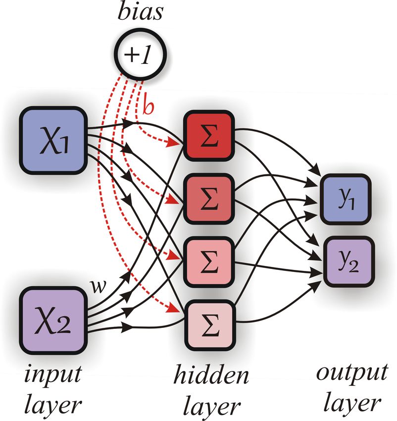
3
ical results for large chains (obtained by density ma-
trix renormalization group methods [42]) in the regime
κ > 1/2. The critical value of g for the Ising transition
for 0 ≤ κ ≤ 1/2 is given approximately by [37]
s
1−κ 1 − 3κ + 4κ 2
gI ( κ ) ≈ 1− . (2)
κ 1−κ
This approximation agrees well with the numerical es-
timates based on exact diagonalization for small chains
[41]. The critical values of g for the CIC and BKT transi-
tions for 1/2 < κ . 3/2 are approximated respectively
by [42]
gCIC (κ ) ≈ 1.05 (κ − 0.5) , (3)
q
gBKT (κ ) ≈ 1.05 (κ − 0.5)(κ − 0.1). (4)
In addition, the paramagnetic phase is sometimes di-
vided into two regions, distinguished by the presence
of commensurate versus incommensurate oscillations
in the exponentially decaying correlations. These two
regions are separated by the exactly known Peschel-
Emery line [48], which does not correspond to a true FIG. 1. Schematic representation of machine learning tech-
phase transition because the energy gap remains finite niques. (a) Supervised learning. (b) Unsupervised learning
and there is no symmetry breaking across this line. The (clustering).
exact expression for the Peschel-Emery line is
1 this recipe, we end up with a myriad of possible ma-
gPE (κ ) = − κ. (5)
4κ chine learning pipelines [1, 2].
While the Ising transition is captured correctly if one In machine learning research, there are two main ap-
only has access to numerical results for short chains, proaches named as supervised and unsupervised learn-
cf. [41], detecting the CIC and BKT transitions using ing, related to the experience passed to the learner.
standard approaches requires computing observables The central difference between them is that supervised
for significantly longer chains [42]. learning is performed with prior knowledge of the cor-
rect output values for a subset of given inputs. In this
case, the objective is to find a function that best approx-
III. MACHINE LEARNING REVIEW imates the relationship between input and output for
the data set. In turn, unsupervised learning, does not
Machine learning is defined as algorithms that iden- have labeled outputs. Its goal is to infer the underly-
tify patterns/relations from data without being specif- ing structure in the data set, in other words, discover
ically programmed to. By using a variety of statisti- hidden patterns in the data, see Fig. 1 for a pictorial
cal/analytical methods, learners improve their perfor- distinction. In this work, in order to propose a general
mance p in solving a task T by just being exposed to framework, we used both approaches in a complemen-
experiences E. Heuristically speaking, machine learn- tary manner.
ing occurs whenever p( T ) ∝ E, i. e. the performance in Using the supervised learning as a prototype, one
solving task T enhances with increasing training data. can depict the general lines of a ML project. We first
The state-of-the-art of a typical ML project has four split the data set into two non-intersecting sets: Xtrain
somewhat independent components: i) the data set X, and Xtest , named training and test sets, respectively.
ii) a model m(w), iii) a cost function J (X; m(w)) and iv) Typically, the test set corresponds to 10% − 30% of the
an optimization procedure. Our aim is to find the best data set. Then, we minimize the cost function with
model parameters, w, which minimizes the cost func- the training set, producing the model, m(w∗ ), where
tion for the given data set. This optimization procedure w∗ = argminw { J (Xtrain ; m(w))}. We evaluate the cost
is, generally, numerical and uses variations of the well function of this model in the test set in order to mea-
known gradient descent algorithm. In this manner, by sure its performance with out-of-sample data. In the
combining distinct ingredients for each component in end, we seek a model that performs adequately in both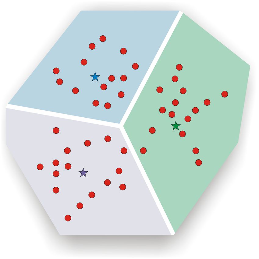
4

sets, i. e., a model that generalizes well. In other words,      IV.   MACHINE LEARNING PHASE TRANSITIONS IN
the model works fine with the data we already have as                          THE ANNNI MODEL
well as with any future data. This quality, called gen-
eralization, is at the core of the difference between the                             A.   Our Data Set
machine learning approach and a simple optimization
solution using the whole data set.                                 We use the pairwise correlations among all spins
                                                                in the lattice as the data set to design our mod-
                                                                els.
                                                                n    Thus, the set ofoobservables used is given by
                                                                             y y
   The performance of the model is made by evaluating             hσix σjx i, hσi σj i, hσiz σjz i with, j > i and i = [1, N − 1]
the cost function in the test set. This is generally done       where N is the number of spins/qubits in the lattice
by computing the mean square error (MSE) between the            and hσix σjx i = hλ0 |σix σjx |λ0 i is the expectation value of
prediction made by the model and the known answer               the spin correlation for the Hamiltonian ground state
(target), etest = h J (Xtest ; m(w∗ ))i. In a ML project, we                                      y y
                                                                |λ0 i (analogously to hσi σj i and hσiz σjz i). It is easy to
are dealing, generally, with complex systems for which
we have a priori no plausible assumption about the un-          see that the number of features is given by 3 ∑kN=−11 k
derlying mathematical model. Therefore, it is common            since that for 8, 10, and 12 sites we have 84, 135, and
to test various types of models (m1 , m2 , ...) and compare     198 features respectively.
their performance on the test set to decide which is the
most suitable one. In fact, it is even possible to combine
them (manually or automatically) in order to achieve                            B.   Unsupervised Approach
better results by reducing bias and variance [1, 2, 26].
                                                                   Unsupervised learning is the branch of machine
                                                                learning dealing with data that has not been labeled,
                                                                classified or categorized. Simply from the features (the
   One should be careful with what is generally called
                                                                components) of the input data, represented by a vec-
overfitting, that is, some models may present small val-
                                                                tor X, one can extract useful properties about it. Quite
ues for etrain , but etest  etrain . It happens because some
                                                                generally, we seek for the entire probability distribution
models (often very complex) can deal well with data
                                                                p(X) that generated and generalizes the data set. Clus-
we already have, however produce large error with un-
                                                                tering the data into groups of similar or related exam-
observed data. Overfitting is a key issue in machine
                                                                ples is a common task in an unsupervised project. Self-
learning and various methods have been developed to
                                                                labeling is another crucial application of unsupervised
reduce the test error, often causing an increase in the
                                                                learning, opening the possibility of combining unsuper-
training error, but reducing the generalization error as
                                                                vised and supervised algorithms to speed up and/or
a whole. Making ensemble of multiple models is one of
                                                                improve the learning process, an approach known as
such techniques and as has been already successfully
                                                                semi-supervised learning (SSL). As we shall demon-
demonstrated [1, 26]. On the opposite trend, we might
                                                                strate, using the ANNNI model as a benchmark, un-
also have underfitting, often happening with very sim-
                                                                supervised learning offers a valuable framework to an-
ple models where etest ∼ etrain are both large. Al-
                                                                alyze complex phase diagrams even in situations where
though extremely important, the discussion about the
                                                                only few and low dimensional input data is available.
bias-variance trade-off is left to the good review in Refs.
                                                                   Briefly describing, the algorithm is used to partition
[1, 2].
                                                                n samples into K clusters, fixed a priori. In this man-
                                                                ner, K centroids are defined, one for each cluster. The
                                                                next step is to associate each point of the data set to
   Overall, the success of a ML project depends on the          the nearest centroid. Having all points associated to a
quality/quantity of available data and also our prior           centroid, we update the centroids to the barycenters of
knowledge about the underlying mechanisms of the                the clusters. So, the K centroids change their position
system. In the Appendix, we provide a brief but intu-           step by step until no more changes are done, i.e. until
itive description of all machine learning steps involved        a convergence is achieved. In other words, centroids do
in our work. These include the tasks (classification            not move more within a predetermined threshold. See
and clustering), the experiences (supervised and un-            Appendix for more details.
supervised learning), the machine learning algorithms              For distinct pairs of the coupling parameters (g; κ) of
(multi-layer perceptron, random forest, and so on) and          the Hamiltonian (1), we explicitly compute all the pair-
also the performance measures. For additional reading           wise spin correlations described in section IV A. Since
and more profound and/or picturesque discussions we             the computation of correlations is computationally very
refer to [1, 2] and as well as to the Appendix.                 expensive, the coupling parameters were varied with
5
FIG. 2. Comparison among the approximate solutions (2) and FIG. 3. Comparison among the approximate solutions (2), (4)
(4) and the unsupervised learning trained N = 12 sites in the and (5) with the unsupervised results for K = 4. As one can
lattice. The Ising transition (2) is almost perfectly reproduced. see, at least qualitatively, the machine is finding a new region
The machine results for the BKT transition (4) shows a smaller associated with the Emery-Peschel line (5).
accuracy; nonetheless, it is qualitatively accurate.
not separate the floating phase and the antiphase but,
step size of 10−2 in the range κ, g ∈ [0, 1]. So, in to- instead, the new critical line that appears for K = 4 di-
tal, we are training the learner with a modest number vides the paramagnetic phase into two regions which,
of 10000 examples. Equipped with that, we investigate at least qualitatively, can be identified with the com-
the capacity of an unsupervised algorithm to retrieve mensurate and incommensurate regions separated by
the phase diagram. In Fig. 2, we show the phase di- the Peschel-Emery line (5). This result is remarkable
agram produced by using k-means algorithm [52] and because it tells us that machine learning approach man-
focusing on a lattice size N = 12. Providing K = 3 ages to detect a subtle change in the correlation func-
to the learner (assuming three phases), the algorithm tions which is hard to discern by conventional methods
returns the best clustering based on the similarities it using only data for small chains, up to N = 12. On the
could find in the features. Strikingly, given the few data other hand, recall that such change in the correlation
points and the relatively small size of spin chain used to function does not correspond to a phase transition in
generated the data, it finds three well distinct clusters the strict sense.
in very good accordance with the three main phases The results presented in this section indicate that un-
of the ANNNI model. Indeed, since we imposed to supervised learning approach is a good candidate when
the method the gathering in only three groups, the K- one knows in advance a good estimate for the number
means algorithm detects the ferromagnetic phase, the of phases K, as it is requested upfront for various un-
paramagnetic phase, and a third one which clustered supervised algorithms. In the next sections, we show
the floating phase with the antiphase. It is quite surpris- how supervised learning can be used as a validation
ing because the boundary between the paramagnetic step for the unsupervised results, also providing sur-
and the floating phases is the BKT transition, there- prisingly accurate results. However, we first address
fore it detects a transition which is notoriously hard to the task of how we can use a complementary unsuper-
pinpoint, as the correlation length diverges exponen- vised approach to cope with the limitation mentioned
tially at the critical point [53]. Moreover, the unsuper- above, that is, when one has no a priori knowledge of a
vised approach almost perfectly recovers the curve cor- reasonable number of existing phases.
responding to the ferromagnetic-paramagnetic transi-
tion and its analytical critical value of gcrit = 1 (with
κ = 0). As well, it gives very accurate quantitative pre-
dictions for the analytical tricritical value κcrit = 1/2, at C. Density-based clustering
which the transition between the ferromagnetic, para-
magnetic and antiphase regions happens. To make our framework applicable to cases in which
We have also tested the unsupervised prediction by we have no guess of how many phases we can possibly
setting K = 4, that is, assuming four phases for the expect, we propose to use a density-based (DB) clus-
ANNNI model as described in Section II. The result is tering technique [54, 55] to estimate an initial number
shown in Fig. (3). As we can see, the algorithm does of clusters. Density clustering makes the intuitive as-6
sumption that clusters are defined by regions of space
with higher density of data points, meaning that out-
liers are expected to form regions of low density. The
main input in such kind of algorithms is the critical dis-
tance e above which a point is taken as an outlier of a
given cluster. In fact, it corresponds to the maximum
distance between two samples for them to be labelled
as in the same neighborhood. One of its most relevant
output is the estimated number of distinct labels, that
is, the number of clusters/phases. Therefore, it can be
taken as a complementary technique for the use of the
k-means or any other unsupervised approach which re-
quires one to specify the number of clusters expected in
the data.
DBSCAN is one of the most common DB clustering
algorithms and is known to deal well with data which
contains clusters of similar density [55], making it suit- FIG. 4. Detecting the critical transverse magnetic field cou-
able for our case. We use DBSCAN to retrieve the num- pling parameter g at which a phase transition occurs. The
ber of clusters we should input in the unsupervised machine was trained at κ = 0 and asked to predict where
KNN algorithm, thus assuming no prior knowledge of the transition happens at κ = 0.1, by considering where the
how many phases one expects. For that, we feed the machine is most uncertain, that is, when the probabilities
DBSCAN with a critical distance e of the order of the p1 = p2 = 1/2. Here the ferromagnetic (paramagnetic) phase
is labeled as 0 (1).
step size used to span the training data, i. e., e = 10−2 .
As a result, the algorithm returned 3 clusters as the
optimal solution, thus coinciding with the three main
In supervised machine learning, the learner experi-
phases present in the ANNNI model, precisely those
ences a data set of features X and also the target or
that one can expect to recognize at the small lattice size
label vector y, provided by a "teacher", hence the term
we have employed. It also coincides with the Elbow
"supervised". In other words, the learner is presented
curve for estimating the optimal number of clusters, see
with example inputs and their known outputs and the
Appendix for details.
aim is to create a general rule that maps inputs to out-
puts, by generally estimating the conditional probabil-
ity p(y|X). One of the main differences between a ML
D. Supervised Approach algorithm and a canonical algorithm is that in the sec-
ond we provide inputs and rules and receive answers
In spite of the clear success of unsupervised ML in and in the first we insert inputs and answers and re-
identifying the phases in the ANNNI model, a natural trieve rules (see Appendix for more details).
question arises. How can we trust the machine predic- Our aim is to understand whether transfer learning
tions in the absence of a more explicit knowledge about is possible (training with κ = 0 to predict at regions
the Hamiltonian under scrutiny? Could partial knowl- where κ ≥ 0). Both the unsupervised approach as
edge help in validating the ML results? Typically, lim- well as the analytical solution to κ = 0, point out that
iting cases of a Hamiltonian of interest are simpler and a transition occurs at g ≈ 1. With this information,
thus more likely to have a known solution. That is pre- we train the supervised algorithms with g ranging in
cisely the case of the ANNNI model, which for κ = 0 the interval [0.5, 1.5]. Given that we don’t have to vary
is fully understood, in particular the fact that at g = 1 over κ, we reduce the step size (in comparison with the
there is a phase transition between the ferromagnetic unsupervised approach) to 10−3 , generating an evenly
and paramagnetic phases. Can a machine trained with distributed training data with equal number of sam-
such limited knowledge (κ = 0) make any meaningful ples, 500 in each phase (ferromagnetic for g < 1 and
predictions to the more general model (κ ≥ 0)? The paramagnetic for g > 1 ). The main drawback of this
best one can hope for in this situation is that the unsu- supervised approach is that it always performs binary
pervised and supervised approaches point out similar classification, known as one-vs-all classification. For in-
solutions, a cross validation enhancing our confidence. stance, for handing writings digits it is similar to the
In the following we show that this is indeed possible by case in which a learner can simply identify whether or
investigating supervised learning algorithms as a com- not the number 5 has been written.
plementary approach to the unsupervised framework Motivated by the sound results in its unsupervised
introduced above. version, we first tried the KNN algorithm (vaguely re-7
TABLE I. Performance (average `1 -norm with relation to the
analytical approximations given by Eqs. 2 and 3) computed
for the three main phases and different ML approaches. See
Appendix for details. Two best ones in boldface.
average `1 -norm
Technique
RF (supervised) 0.03375(9)
KNN (supervised) 0.07461(4)
MLP (supervised) 0.18571(4)
XGB (supervised) 0.19507(7)
KNN (unsupervised - 12 sites) 0.03474(4)
KNN (unsupervised - 8 sites) 0.07904(1)
KNN (unsupervised - 10 sites) 0.16350(2)
the models were never trained for the antiphase, it is
a good test to check the learner’s ability to classify a
FIG. 5. Phase diagrams produced with diverse ML algo-
new phase as an outlier. For κ ≥ 0.5, we are in a region
rithms when trained only with κ = 0: KNN (black circles), where only phases ’0’ and ’2’ are present. So, the best
Random Forest (cyan down stars), Multilayer Perceptron (yel- the machine model can do is to output ’0’ fs the phase is
low squares) and Extreme Gradient Boosting (blue diagonal indeed ’0’ and ’1’ otherwise. As we already remarked,
stars) and two different analytical solutions (Ising (solid blue) it is a drawback of the supervised approach in com-
and BKT (solid orange triangles). All different methods re- parison to the unsupervised one, but it is still useful to
cover the ferro/paramagnetic transition very well while the validate the emergence of a new phase, as suggested
transition between the paragmanetic and the BKT are only re- by the unsupervised technique. In this sense, the KNN
covered by the KNN and RF methods (see main text for more and RF methods perform quite well. As seen in Fig. 5
details).
the transition between the paramagnetic and the clus-
tered antiphase/floating is qualitatively recovered even
though the machine has never been exposed to these
lated to the k-means method) as well as different meth- phases before.
ods such as the multilayer perceptron (MLP, a deep In Table 1 we present the average `1 -norm for the dis-
learning algorithm), random forest (RF) and extreme tinct algorithms taking as benchmark the approximate
gradient boosting (XGB). Once the model is trained, we analytical solutions for the three main phases given
use the same data set used in section IV B to predict the by Eqs. (2) and (4). One can observe that the two
corresponding phases. Actually, for a given instance best approaches are the supervised RF and the unsu-
0 0
X , the trained model, m, returns m( X ) = ( p1 , p2 ), pervised KNN trained with 12 sites, which reinforces
where ( p1 , p2 ) is a normalized probability vector and our framework of using the unsupervised and super-
the assigned phase corresponds to the component with vised methodologies complementarily. It is worth men-
largest value. To determine when we are facing a tran- tioning that the better performance of the supervised
sition, we plot both the probability components and approach is related to the fact that we provided more
check when they cross, as shown in Fig. 4. As can be training data, accounting for a more precise transition,
seen in Fig. 5, the different ML methods successfully as the step size over g is reduced.
recover the left part (κ < 0.5) of the phase diagram, ex-
actly corresponding to the ferromagnetic/paramagnetic
transition over which the machine has be trained for the V. DISCUSSION
case κ = 0. However, what happens as we approach the
tricritical point at κ = 0.5 at which new phases (the an- In this paper we have proposed a machine learn-
tiphase and the floating phase) appears? As can be seen ing framework to analyze the phase diagram and
in Fig. 5, near this point the predictions of the different phase transitions of quantum Hamiltonians. Taking
methods start to differ. the ANNNI model as a benchmark, we have shown
To understand what is going on, we highlight that how the combination of a variety of ML methods can
since the machine can only give one out of two an- characterize, both qualitatively and quantitatively, the
swers (the ones it has been trained for), the best it can complex phases appearing in this Hamiltonian. First,
do is to identify the clustered antiphase/floating phase we demonstrated how the unsupervised approach can
(here labeled as phase ’2’) with either the ferromagnetic recover accurate predictions about the 3 main phases
(phase ’0’) or the paramagnetic (phase ’1’) cases. Since (ferromagnetic, paramagnetic and the clustered an-8
tiphase/floating) of the ANNNI model. It can also re- Overall, we see that both the unsupervised and the
cover qualitatively different regions within the param- various supervised machine learning predictions are in
agnetic phase as described by the Emery-Peschel line, very good agreement. Not only do they recover simi-
even though there is no true phase transition in the lar critical lines but also discover the multicritical point
thermodynamic limit. This is remarkable, given that of the phase diagram. Clearly, we can only say that
typically this transition needs large lattice sizes to be ev- because the precise results are known for the ANNNI
idenced. Here, however, we achieve that using compar- model. The general problem of mapping out phase
atively very small lattice sizes (up to 12 spins). Finally, diagrams of quantum many-body systems is still very
we have also considered supervised/transfer learning much open, even more so with the discovery of topo-
and showed how transfer learning becomes possible: by logical phases. The methods investigated here may con-
training the machine at κ = 0 (κ representing the next- tribute to advancing this field and hope to motivate the
neighbour interaction strength) we can also accurately application of this framework to Hamiltonians where
determine the phase transitions happening at κ ≥ 0. the different phases have not yet been completely sorted
Surprisingly, the machine trained to distinguish the fer- out. If as it happens for the ANNNI model, if all these
romagnetic and paramagnetic phase is also able to iden- multitude of evidence obtained by considerably differ-
tify the BKT transition, which is notoriously hard to ent ML methods point out similar predictions, this ar-
pinpoint, since the correlation length diverges exponen- guably give us good confidence about the correctness
tially at the critical point. Moreover, we note that the of the results. The predictions given by the ML ap-
machine is not simply testing the order parameter be- proach we propose here can be seen as guide, an initial
cause it is able to distinguish between the ferromagnetic educated guess of regions in the space of physical pa-
phase and the antiphase which are both ordered but rameters where phase transitions could be happening.
with a different order parameter. Indeed, the machine ACKNOWLEDGEMENTS
is identifying a new pattern in the data.
Taken together, these results suggest that the ML in-
vestigation should start with the unsupervised tech-
niques (DBSCAN + Clustering), as it is a great initial The authors acknowledge the Brazilian ministries
exploratory entry point in situations where it is either MEC and MCTIC, funding agency CNPq (AC’s Uni-
impossible or impractical for a human or an ordinary versal grant No. 423713/2016 − 7, RC’s grants No.
algorithm to propose trends and/or have insights with 307172/2017 − 1 and No406574/2018 − 9 and INCT-IQ)
the raw data. After some hypotheses are collected with and UFAL (AC’s paid license for scientific cooperation
the unsupervised approach, one should now proceed at UFRN). This work was supported by the Serrapil-
to get more data and apply supervised techniques as to heira Institute (grant number Serra-1708-15763) and the
consolidate the unsupervised outputs. See Appendix John Templeton Foundation via the grant Q-CAUSAl
for more discussions. No 61084.
[1] Ian Goodfellow, Yoshua Bengio, and Aaron [7] Frank Rosenblatt, “The perceptron: a probabilistic model
Courville, Deep Learning (MIT Press, 2016) for information storage and organization in the brain.”
http://www.deeplearningbook.org. Psychological review 65, 386 (1958).
[2] Pankaj Mehta, Marin Bukov, Ching-Hao Wang, Alexan- [8] Randal S. Olson, Nathan Bartley, Ryan J. Urbanowicz,
dre G. R. Day, Clint Richardson, Charles K. Fisher, and Jason H. Moore, “Evaluation of a tree-based pipeline
and David J. Schwab, “A high-bias, low-variance in- optimization tool for automating data science,” in Pro-
troduction to machine learning for physicists,” (2018), ceedings of the Genetic and Evolutionary Computation Confer-
arXiv:1803.08823. ence 2016, GECCO ’16 (ACM, New York, NY, USA, 2016)
[3] Leo Breiman, “Random forests,” Machine learning 45, 5– pp. 485–492.
32 (2001). [9] Diederik P. Kingma and Jimmy Ba, “Adam: A method
[4] Naomi S Altman, “An introduction to kernel and for stochastic optimization.” CoRR abs/1412.6980 (2014).
nearest-neighbor nonparametric regression,” The Amer- [10] Pierre Geurts, Damien Ernst, and Louis Wehenkel, “Ex-
ican Statistician 46, 175–185 (1992). tremely randomized trees,” Mach. Learn. 63, 3–42 (2006).
[5] L Breiman, JH Friedman, RA Olshen, and CJ Stone, [11] X. Qiu, L. Zhang, Y. Ren, P. N. Suganthan, and G. Ama-
“Classification and regression trees, 1984: Belmont,” CA: ratunga, “Ensemble deep learning for regression and
Wadsworth International Group (1984). time series forecasting,” in 2014 IEEE Symposium on Com-
[6] Pierre Geurts, Damien Ernst, and Louis Wehenkel, “Ex- putational Intelligence in Ensemble Learning (CIEL) (2014)
tremely randomized trees,” Machine learning 63, 3–42 pp. 1–6.
(2006). [12] David E Rumelhart, Geoffrey E Hinton, and
Ronald J Williams, “Learning representations by back-9
propagating errors,” nature 323, 533 (1986). arXiv:1808.07069.
[13] M. I. Jordan and T. M. Mitchell, “Machine learning: [27] Raban Iten, Tony Metger, Henrik Wilming, Lídia Del Rio,
Trends, perspectives, and prospects,” Science 349, 255– and Renato Renner, “Discovering physical concepts
260 (2015). with neural networks,” arXiv preprint arXiv:1807.10300
[14] Harshil M Kamdar, Matthew J Turk, and Robert J Brun- (2018).
ner, “Machine learning and cosmological simulations–i. [28] Giuseppe Carleo and Matthias Troyer, “Solving the
semi-analytical models,” Monthly Notices of the Royal quantum many-body problem with artificial neural net-
Astronomical Society 455, 642–658 (2015). works,” Science 355, 602–606 (2017).
[15] Harshil M Kamdar, Matthew J Turk, and Robert J Brun- [29] Giacomo Torlai and Roger G Melko, “Learning thermo-
ner, “Machine learning and cosmological simulations– dynamics with boltzmann machines,” Physical Review B
ii. hydrodynamical simulations,” Monthly Notices of the 94, 165134 (2016).
Royal Astronomical Society 457, 1162–1179 (2016). [30] Luca M Ghiringhelli, Jan Vybiral, Sergey V Levchenko,
[16] John D Kelleher, Brian Mac Namee, and Aoife D’Arcy, Claudia Draxl, and Matthias Scheffler, “Big data of ma-
Fundamentals of machine learning for predictive data ana- terials science: critical role of the descriptor,” Physical
lytics: algorithms, worked examples, and case studies (MIT review letters 114, 105503 (2015).
Press, 2015). [31] Juan Carrasquilla and Roger G. Melko, “Machine learn-
[17] Michelle Lochner, Jason D McEwen, Hiranya V Peiris, ing phases of matter,” Nature Physics 13, 431–434 (2017).
Ofer Lahav, and Max K Winter, “Photometric supernova [32] Peter Broecker, Juan Carrasquilla, Roger G Melko, and
classification with machine learning,” The Astrophysical Simon Trebst, “Machine learning quantum phases of
Journal Supplement Series 225, 31 (2016). matter beyond the fermion sign problem,” Scientific re-
[18] Tom Charnock and Adam Moss, “supernovae: Photo- ports 7, 8823 (2017).
metric classification of supernovae,” Astrophysics Source [33] Kelvin Ch’ng, Juan Carrasquilla, Roger G. Melko, and
Code Library (2017). Ehsan Khatami, “Machine learning phases of strongly
[19] Rahul Biswas, Lindy Blackburn, Junwei Cao, Reed Es- correlated fermions,” Phys. Rev. X 7, 031038 (2017).
sick, Kari Alison Hodge, Erotokritos Katsavounidis, [34] Dong-Ling Deng, Xiaopeng Li, and S Das Sarma, “Ma-
Kyungmin Kim, Young-Min Kim, Eric-Olivier Le Bigot, chine learning topological states,” Physical Review B 96,
Chang-Hwan Lee, et al., “Application of machine learn- 195145 (2017).
ing algorithms to the study of noise artifacts in [35] Patrick Huembeli, Alexandre Dauphin, and Peter Wit-
gravitational-wave data,” Physical Review D 88, 062003 tek, “Identifying quantum phase transitions with adver-
(2013). sarial neural networks,” Physical Review B 97, 134109
[20] M Carrillo, JA González, M Gracia-Linares, and (2018).
FS Guzmán, “Time series analysis of gravitational wave [36] W Selke, “The ANNNI model — theoretical analysis and
signals using neural networks,” in Journal of Physics: Con- experimental application,” Physics Reports 170, 213–264
ference Series, Vol. 654 (IOP Publishing, 2015) p. 012001. (1988).
[21] Adam Gauci, Kristian Zarb Adami, and John Abela, [37] Sei Suzuki, Jun ichi Inoue, and Bikas K. Chakrabarti,
“Machine learning for galaxy morphology classifica- Quantum Ising Phases and Transitions in Transverse Ising
tion,” arXiv preprint arXiv:1005.0390 (2010). Models (Springer Berlin Heidelberg, 2013).
[22] Nicholas M Ball, Jon Loveday, Masataka Fukugita, Os- [38] J. Villain and P. Bak, “Two-dimensional ising model with
amu Nakamura, Sadanori Okamura, Jon Brinkmann, competing interactions : floating phase, walls and dislo-
and Robert J Brunner, “Galaxy types in the sloan digital cations,” Journal de Physique 42, 657–668 (1981).
sky survey using supervised artificial neural networks,” [39] D Allen, P Azaria, and P Lecheminant, “A two-leg quan-
Monthly Notices of the Royal Astronomical Society 348, tum ising ladder: a bosonization study of the ANNNI
1038–1046 (2004). model,” Journal of Physics A: Mathematical and General
[23] Manda Banerji, Ofer Lahav, Chris J Lintott, Filipe B Ab- 34, L305–L310 (2001).
dalla, Kevin Schawinski, Steven P Bamford, Dan An- [40] Heiko Rieger and Genadi Uimin, “The one-dimensional
dreescu, Phil Murray, M Jordan Raddick, Anze Slosar, ANNNI model in a transverse field: analytic and nu-
et al., “Galaxy zoo: reproducing galaxy morphologies via merical study of effective hamiltonians,” Zeitschrift für
machine learning,” Monthly Notices of the Royal Astro- Physik B Condensed Matter 101, 597–611 (1996).
nomical Society 406, 342–353 (2010). [41] Paulo R. Colares Guimarães, João A. Plascak, Fran-
[24] CE Petrillo, C Tortora, S Chatterjee, G Vernardos, LVE cisco C. Sá Barreto, and João Florencio, “Quantum
Koopmans, G Verdoes Kleijn, NR Napolitano, G Covone, phase transitions in the one-dimensional transverse ising
P Schneider, A Grado, et al., “Finding strong gravitational model with second-neighbor interactions,” Phys. Rev. B
lenses in the kilo degree survey with convolutional neu- 66, 064413 (2002).
ral networks,” Monthly Notices of the Royal Astronomi- [42] Matteo Beccaria, Massimo Campostrini, and Alessan-
cal Society (2017). dra Feo, “Evidence for a floating phase of the transverse
[25] Giacomo Torlai, Guglielmo Mazzola, Juan Carrasquilla, annni model at high frustration,” Phys. Rev. B 76, 094410
Matthias Troyer, Roger Melko, and Giuseppe Carleo, (2007).
“Neural-network quantum state tomography,” Nature [43] Adam Nagy, “Exploring phase transitions by finite-
Physics 14, 447 (2018). entanglement scaling of MPS in the 1d ANNNI model,”
[26] Askery Canabarro, Samuraí Brito, and Rafael Chaves, New Journal of Physics 13, 023015 (2011).
“Machine learning non-local correlations,” (2018),10
[44] J.-J. Wen, W. Tian, V. O. Garlea, S. M. Koohpayeh, T. M. APPENDIX
McQueen, H.-F. Li, J.-Q. Yan, J. A. Rodriguez-Rivera,
D. Vaknin, and C. L. Broholm, “Disorder from or-
A. The experience E: supervised and unsupervised
der among anisotropic next-nearest-neighbor ising spin
learning
chains in srho2 o4 ,” Phys. Rev. B 91, 054424 (2015).
[45] C. Karrasch and D. Schuricht, “Dynamical phase transi-
tions after quenches in nonintegrable models,” Phys. Rev. Within machine learning research, there are two ma-
B 87, 195104 (2013). jor methods termed as supervised and unsupervised
[46] Fabian Hassler and Dirk Schuricht, “Strongly interact- learning. In a nutshell, the key difference between them
ing majorana modes in an array of josephson junctions,” is that supervised learning is performed using a first-
New Journal of Physics 14, 125018 (2012). hand information, i. e., one has ("the teacher", hence
[47] A. Milsted, L. Seabra, I. C. Fulga, C. W. J. Beenakker, and
the term "supervised") prior knowledge of the output
E. Cobanera, “Statistical translation invariance protects a
values for all and every input samples. Here, the ob-
topological insulator from interactions,” Phys. Rev. B 92,
085139 (2015). jective is to find/learn a function that best ciphers the
[48] I. Peschel and V. J. Emery, “Calculation of spin cor- relationship between input and output. In contrast, un-
relations in two-dimensional ising systems from one- supervised learning deals with unlabeled outputs and
dimensional kinetic models,” Zeitschrift für Physik B its goal is to infer the natural structure present within
Condensed Matter 43, 241–249 (1981). the data set.
[49] Thierry Giamarchi, Quantum physics in one dimension, In- In a supervised learning project, the learner experi-
ternat. Ser. Mono. Phys. (Clarendon Press, Oxford, 2004). ences data points of features X and also the correspond-
[50] Subir Sachdev, Quantum Phase Transitions (Cambridge
ing target or label vector y, aiming to create a univer-
University Press, 2009).
sal rule that maps inputs to outputs, by generally esti-
[51] H. J. Schulz, “Critical behavior of commensurate-
incommensurate phase transitions in two dimensions,” mating the conditional probability p(y|X). Typical su-
Phys. Rev. B 22, 5274–5277 (1980). pervised learning tasks are: (i) classification, when one
[52] J. MacQueen, “Some methods for classification and anal- seeks to map input to discrete output (labels), or (ii) re-
ysis of multivariate observations,” in Proceedings of the gression, when one wants to map input to a continuous
Fifth Berkeley Symposium on Mathematical Statistics and output set. Common supervised learning algorithms
Probability, Volume 1: Statistics (University of California include: Logistic Regression, Naive Bayes, Support Vec-
Press, Berkeley, Calif., 1967) pp. 281–297. tor Machines, Decision Tree, Extreme Gradient Boosting
[53] J. M. Kosterlitz and D. J. Thouless, “Ordering, metastabil- (XGB), Random Forests and Artificial Neural Networks.
ity and phase transitions in two-dimensional systems,” J. Later, we provide more details of the ones used in this
Phys. C6, 1181–1203 (1973), [,349(1973)].
work.
[54] Hans-Peter Kriegel, Peer Kröger, Jörg Sander,
and Arthur Zimek, “Density-based clustering,” In unsupervised learning, as there is no teacher to
Wiley Interdisciplinary Reviews: Data Mining label, classify or categorize the input data, the learner
and Knowledge Discovery 1, 231–240 (2011), must grasp by himself how to deal with the data. Sim-
https://onlinelibrary.wiley.com/doi/pdf/10.1002/widm.30. ply from the features (the components) of the input
[55] Martin Ester, Hans-Peter Kriegel, Jörg Sander, and Xi- data, represented by a vector X, one can extract use-
aowei Xu, “A density-based algorithm for discovering ful properties about it. Quite generally, we seek for
clusters in large spatial databases with noise,” (AAAI the entire probability distribution p(X) that generated
Press, 1996) pp. 226–231. and generalizes the data set, as we have pointed out
[56] Y. Bengio, A. Courville, and P. Vincent, “Representation
in the main text. The most usual tasks of an unsu-
learning: A review and new perspectives,” IEEE Trans-
actions on Pattern Analysis and Machine Intelligence 35,
pervised learning project are: (i) clustering, (ii) repre-
1798–1828 (2013). sentation learning [56] and dimension reduction, and
[57] J. MacQueen, “Some methods for classification and anal- (iii) density estimation. Although we focus on cluster-
ysis of multivariate observations,” in Proceedings of the ing in this work, in all of these tasks, we aim to learn
Fifth Berkeley Symposium on Mathematical Statistics and the innate structure of our unlabelled data. Some pop-
Probability, Volume 1: Statistics (University of California ular algorithms are: K-means for clustering; Principal
Press, Berkeley, Calif., 1967) pp. 281–297. Component Analysis (PCA) and autoencoders for rep-
[58] F. Pedregosa, G. Varoquaux, A. Gramfort, V. Michel, resentation learning and dimension reduction; and Ker-
B. Thirion, O. Grisel, M. Blondel, P. Prettenhofer, nel Density Estimation for density estimation. Since
R. Weiss, V. Dubourg, J. Vanderplas, A. Passos, D. Cour-
no labels are given, there is no specific way to com-
napeau, M. Brucher, M. Perrot, and E. Duchesnay,
pare model performance in most unsupervised learn-
“Scikit-learn: Machine learning in Python,” Journal of
Machine Learning Research 12, 2825–2830 (2011). ing methods. In fact, it is even hard to define tech-
[59] Jerome H. Friedman, “Greedy function approximation: nically Unsupervised Learning, check [1, 2] for deeper
A gradient boosting machine,” Annals of Statistics 29, discussions.
1189–1232 (2000). As briefly mentioned in the main text, unsupervised11
learning is very useful in exploratory analysis and in- 2. Clustering
tegrated many ML pipelines once it can automatically
identify structure in data. For example, given the task Clustering is one of the most important unsupervised
of labelling or inserting caption for the tantamount of learning problem. As the other problems of this ap-
images available on the world web, unsupervised meth- proach, it aims to identify a structure in the unlabelled
ods would be (and in fact is) a great starting point for data set. A loose definition of clustering could be “the
this task, as those used by Google’s Conceptual Cap- process of organizing objects into groups whose mem-
tions Team. In situations like this, it is impossible or bers are similar in some way”. A cluster is therefore a
at least impractical for a human or even a regular algo- collection of objects which are “similar” between them
rithm to perform such task. and are “dissimilar” to the objects belonging to other
Machine learning is a method used to build com- clusters. Later in this Appendix, we provide more de-
plex models to make predictions in problems difficult tail about k-means as well as density-based clustering.
to solve with conventional programs. It may as well However, for a more technical definition, please check
shed new light on how intelligence works. However, it Ref. [54]. For a formal mathematical description, we
is worth mentioning that this is not, in general, the main refer the reader to Ref. [57].
purpose behind machine learning techniques given that
by "learning" it is usually meant the skill to perform the
task better and better, not necessarily how it is learning C. The performance p
the task itself. For instance, in a binary classification
task, e. g., "cat vs dog", the program does not learn One important aspects of supervised learning which
what a dog is in the same sense as human does, but it makes it different from an optimization algorithm is
learns how to differentiate it from a cat. In this manner, generalization, as mentioned in section III. It means that
it only learns the following truisms: (i) a dog is a dog we project the algorithm to perform well both on seen
and (ii) a dog is not a cat (and similar statements for (train set) and unseen (test set) inputs. This is accom-
what a cat is). Also, it is important to emphasize that plished by measuring the performance on both the sets.
a highly specialized learning process does not imply, The test set normally corresponds to 10% − 30% of the
necessarily, a better instruction. For example, a more available data.
flexible process may, in fact, be more efficient to achieve For a binary classification tasks (as the ones we dealt
an efficient transfer learning. with in this work), one practical measure is the accu-
racy score which is the proportion of correct predictions
produced by the algorithm. For the classification task
B. Tasks: classification and clustering in this work, we were satisfied with a specific model,
i. e. the model was taken to be optimal, when both
the train and test sets accuracy score were higher than
A machine learning task is specified by how the
99.5%. It is worth mentioning that we used these well-
learner process a given set of input data X ∈ Rn . Some
trained models for κ = 0 when we seek to achieve an
usual ML tasks are: classification, regression, cluster-
efficient transfer learning. In other words, when we
ing, transcription, machine translation, anomaly detec-
tried to used these models for κ > 0
tion, and so on. Here, we quickly describe the two kinds
of tasks we use in this work: classification and cluster- As already addressed in the main text, the opti-
ing. mal model is found by minimizing a cost function.
However, the ideal cost function varies from project to
project and from algorithm to algorithm. For all super-
vised techniques, we used the default cost function of
1. Classification the Python scikit-learn package for the implementation
of a given algorithm [58]. Therefore, we present the cost
Here, the program must designate in which class functions case by case in the next subsection. However,
an input instance should be classified, given K pos- to present the performance in Table I, we use the L1 er-
sible categories. The algorithm retrieves a function ror due to its straightforward interpretation for model
f : Rn → {1, ..., k}, where K is a finite and commonly comparison.
pre-set integer number. So, for a given input vector X,
the model returns a target vector y = f (X). Typically, f
returns a normalized probability distribution over the D. Algorithms
K classes and the proposed class is that with highest
probability. Referring to the main text, this is the case All algorithms used in this work are native to the
for all the supervised algorithms. Python Scikit-Learn package, see Ref. [58] for more de-12
tails. Here, we provide a description of the used meth- happens to be the variance. Formally, the objective is to
ods, highlighting the parameters and hyper-parameters find:
used to calibrate the models and consequently generate
the figures. k k
arg min ∑ ∑ kx − µi k2 = arg min ∑ |Si | Var Si , (6)
S i = 1 x ∈ Si S i =1
1. k-means clustering
where µ j is the mean of the points in Si . This is equiv-
The k-means is an unsupervised learning algorithm. alent to minimizing the pairwise squared deviations of
It searches for k clusters within an unlabeled multidi- points in the same cluster:
mensional data set, where the centers of the clusters
are taken to be the arithmetic mean of all the points k
1
belonging to the respective cluster, hence the term k- arg min ∑ ∑ k x − y k2 . (7)
S i =1
2 | Si | x,y∈Si
means. Clustering stands for finding groups of simi-
lar objects while keeping dissimilar objects in different
The algorithm runs as follows: (1) (randomly) initial-
groups [54]. When convergence is reached, each point
ize the k clusters centroids µ j ; (2) [repeat until conver-
is closer to its own cluster center than to other cluster
centers. It can be seen as a vector quantization (discrete gence] a) for every observation Xi assign it to the near-
output), once its final product it to assert labels to the est cluster; b) update the cluster centroid. Check [57] for
entire data set. detailed mathematical demonstration of asymptotic be-
havior and convergence. Intuitively, one seeks to min-
The data set is, generally, a set of d-dimensional real-
imize the within-group dissimilarity and maximize the
valued points sampled from some unknown probability
between-group dissimilarity for a predefined number
distribution and the dissimilarity function is often the
of clusters k and dissimilarity function. From a statis-
Euclidean distance. k-means clustering aims to parti-
tical perspective, this approach can be used to retrieve
tion n observations into k clusters in which each ob-
k probability densities pi . Assuming that they belong
servation belongs to the cluster with the nearest mean,
to the same parametric family (Gaussian, Cauchy, and
serving as a prototype of the cluster and providing a
so on), one can take the unknown distribution p as a
meaningful grouping of the data set. This results in
mixture of the k distribution pi , as depicted in figure 2
a partitioning of the data space into Voronoi cells, as
(b).
schematically represented in Fig. 6.
We have used the library sklearn.cluster.KMeans which
uses some new initialization technique for speeding up
the convergence time. The main input parameter is the
number of clusters. Overall, k-means is a very fast algo-
rithm. Check the library for the details and the default
parameters [58].
2. Density-based (DB) clustering
In density-based clustering methods the clusters are
taken to be high-density regions of the probability dis-
tribution, giving reason for its name [54]. Here, the
number of clusters is not required as an input parame-
ter. Also, the unknown probability function is not con-
sidered a mixture of the probability functions of the
clusters. It is said to be a nonparametric approach.
Heuristically, DB clustering corresponds to partitioning
group of high density points (core points) separated by
contiguous region of low density points (outliers).
FIG. 6. Schematic representation of the k-means clustering. In this work, we used the Density-Based Spatial
Clustering (DBSCAN) using the scikit-learn package
Given a set of n observations ( X1 , X2 , ..., Xn ), where sklearn.cluster.DBSCAN. The algorithm is fast and very
Xi ∈ Rd , k-means clustering seeks to partition the n good for data set which contains clusters of similar den-
observations into k (k ≤ n) sets S = S1 , S2 , ..., Sk so as sity [58]. The most important input parameter is the
to minimize the within-cluster sum of squares, which maximum distance between two points for them to beYou can also read