Using Twitter Attribute Information to Predict Stock Prices - arXiv
←
→
Page content transcription
If your browser does not render page correctly, please read the page content below
Using Twitter Attribute
                                                         Information to Predict
                                                         Stock Prices
arXiv:2105.01402v1 [cs.LG] 4 May 2021

                                                         Roderick Karlemstrand
                                                           Ebba Leckström
                                        School of Electrical Engineering and Computer Science
                                                   KTH Royal Institute of Technology

                                                       Supervisor: Bengt Pramborg
                                                        Examiner: Anders Västberg

                                                       A Thesis Submitted for the Degree of
                                        Bachelor of Engineering in Electronics and Computer Engineering,
                                        Bachelor of Science in Information and Communication Technology
                                                                Stockholm, 2021
Copyright © 2019 – 2021 Roderick Karlemstrand & Ebba Leckström
All rights reserved. The figures and images in this thesis may not be reused,
reproduced, adapted or redrawn.

”Sometimes when you innovate, you make mistakes. It is best to admit
them quickly and get on with improving your other innovations.”

                                                       — Steve Jobs

                                 i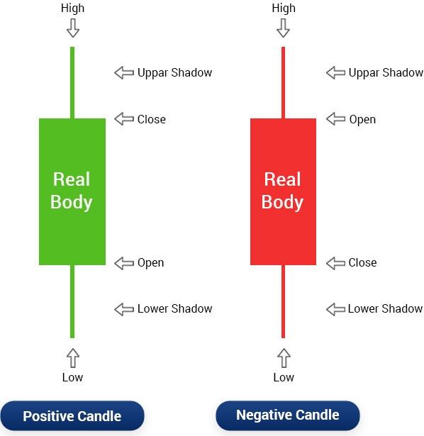
Abstract
Being able to predict stock prices might be the unspoken wish of stock in-
vestors. Although stock prices are complicated to predict, there are many
theories about what affects their movements, including interest rates, news
and social media. With the help of Machine Learning, complex patterns
in data can be identified beyond the human intellect. In this thesis, a Ma-
chine Learning model for time series forecasting is created and tested to
predict stock prices. The model is based on a neural network with several
layers of Long Short-Term Memory (LSTM) and fully connected layers.
It is trained with historical stock values, technical indicators and Twit-
ter attribute information retrieved, extracted and calculated from posts on
the social media platform Twitter. These attributes are sentiment score,
favourites, followers, retweets and if an account is verified. To collect data
from Twitter, Twitter’s API is used. Sentiment analysis is conducted with
Valence Aware Dictionary and sEntiment Reasoner (VADER). The re-
sults show that by adding more Twitter attributes, the Mean Squared
Error (MSE) between the predicted prices and the actual prices improved
by 3%. With technical analysis taken into account, MSE decreases from
0.1617 to 0.1437, which is an improvement of around 11%. The restrictions
of this study include that the selected stock has to be publicly listed on
the stock market and popular on Twitter and among individual investors.
Besides, the stock markets’ opening hours differ from Twitter, which con-
stantly available. It may therefore introduce noises in the model.

Keywords: Stock price prediction, Machine Learning, Deep Learning,
Time series prediction, Twitter, Twitter attributes

                                      ii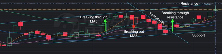
Sammanfattnning
Att kunna förutspå aktiekurser kan sägas vara aktiespararnas outtalade
önskan. Även om aktievärden är komplicerade att förutspå finns det många
teorier om vad som påverkar dess rörelser, bland annat räntor, nyheter och
sociala medier. Med hjälp av maskininlärning kan mönster i data iden-
tifieras bortom människans intellekt. I detta examensarbete skapas och
testas en modell inom maskininlärning i syfte att beräkna framtida ak-
tiepriser. Modellen baseras på ett neuralt nätverk med flera lager av LSTM
och fullt kopplade lager. Den tränas med historiska aktievärden, tekniska
indikatorer och Twitter-attributinformation. De är hämtad, extraherad och
beräknad från inlägg på den sociala plattformen Twitter. Dessa attribut är
sentiment-värde, antal favorit-markeringar, följare, retweets och om kontot
är verifierat. För att samla in data från Twitter används Twitters API och
sentimentanalys genomförs genom VADER. Resultatet visar att genom
att lägga till fler Twitter attribut förbättrade MSE mellan de förutspådda
värdena och de faktiska värdena med 3%. Genom att ta teknisk analys
i beaktande minskar MSE från 0,1617 till 0,1437, vilket är en förbättring
på 11%. Begränsningar i denna studie innefattar bland annat att den ut-
valda aktien ska vara publikt listad på börsen och populär på Twitter och
bland småspararna. Dessutom skiljer sig aktiemarknadens öppettider från
Twitter då den är ständigt tillgänglig. Detta kan då introducera brus i
modellen.

                                      iii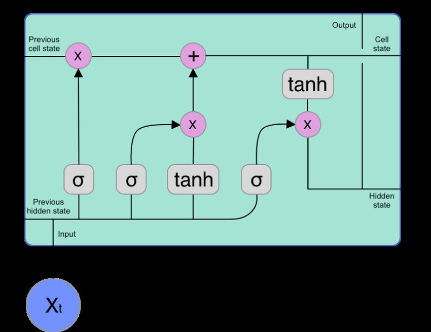
Acknowledgement
We would like to express our special thanks of gratitude to Prof. Anders
Västberg for the guidance in this project as well as Dr Bengt Pramborg for
providing comments and suggestions to help us write this thesis. Without
them, this thesis would not be possible. Secondly, we would like to thank
our families. We are extremely grateful for their love, understanding, car-
ing and support. We are also thankful for the help from Eva Boström and
Hans Förnestig. Last but not the least, we want to thank Maria Wäppling,
Serge de Gosson de Varennes, Hampus Pettersson and Fredrik Schalling
from Sopra Steria for their feedback and help.

5 April 2021
Stockholm, Sweden

                                    iv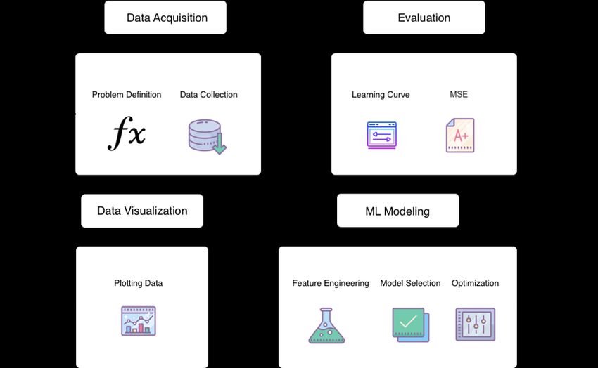
Contents

1 Introduction                                                                                                                            1
  1.1 Background . . . . . . . . . . . . . .                          .   .   .   .   .   .   .   .   .   .   .   .   .   .   .   .   .   2
  1.2 Problem . . . . . . . . . . . . . . . .                         .   .   .   .   .   .   .   .   .   .   .   .   .   .   .   .   .   2
  1.3 Purpose . . . . . . . . . . . . . . . .                         .   .   .   .   .   .   .   .   .   .   .   .   .   .   .   .   .   4
  1.4 Goals . . . . . . . . . . . . . . . . . .                       .   .   .   .   .   .   .   .   .   .   .   .   .   .   .   .   .   4
  1.5 Research Methods and Methodology                                .   .   .   .   .   .   .   .   .   .   .   .   .   .   .   .   .   6
  1.6 Delimitations . . . . . . . . . . . . .                         .   .   .   .   .   .   .   .   .   .   .   .   .   .   .   .   .   6
  1.7 Diposition . . . . . . . . . . . . . . .                        .   .   .   .   .   .   .   .   .   .   .   .   .   .   .   .   .   7

2 Background                                                                                                                               8
  2.1 Related Work . . .      .   .   .   .   .   .   .   .   .   .   .   .   .   .   .   .   .   .   .   .   .   .   .   .   .   .   .    8
  2.2 Twitter . . . . . .     .   .   .   .   .   .   .   .   .   .   .   .   .   .   .   .   .   .   .   .   .   .   .   .   .   .   .   10
  2.3 Sentiment Analysis      .   .   .   .   .   .   .   .   .   .   .   .   .   .   .   .   .   .   .   .   .   .   .   .   .   .   .   11
  2.4 Machine Learning .      .   .   .   .   .   .   .   .   .   .   .   .   .   .   .   .   .   .   .   .   .   .   .   .   .   .   .   12
  2.5 Technical Analysis      .   .   .   .   .   .   .   .   .   .   .   .   .   .   .   .   .   .   .   .   .   .   .   .   .   .   .   18

3 Methods                                                                                                                                 23
  3.1 Choice of methods . . . . . . .                     .   .   .   .   .   .   .   .   .   .   .   .   .   .   .   .   .   .   .   .   23
  3.2 Development Environment . . .                       .   .   .   .   .   .   .   .   .   .   .   .   .   .   .   .   .   .   .   .   25
  3.3 Data Collection by Twitter API                      .   .   .   .   .   .   .   .   .   .   .   .   .   .   .   .   .   .   .   .   25
  3.4 Data Processing . . . . . . . . .                   .   .   .   .   .   .   .   .   .   .   .   .   .   .   .   .   .   .   .   .   27
  3.5 Neural Network Model . . . . .                      .   .   .   .   .   .   .   .   .   .   .   .   .   .   .   .   .   .   .   .   28
  3.6 Evaluation of Model . . . . . .                     .   .   .   .   .   .   .   .   .   .   .   .   .   .   .   .   .   .   .   .   31

4 Results                                                                                                                                 32
  4.1 Data Collection . . . .         . . . . .           .   .   .   .   .   .   .   .   .   .   .   .   .   .   .   .   .   .   .   .   32
  4.2 Feature Engineering . .         . . . . .           .   .   .   .   .   .   .   .   .   .   .   .   .   .   .   .   .   .   .   .   33
  4.3 Training of The Neural          Network             .   .   .   .   .   .   .   .   .   .   .   .   .   .   .   .   .   .   .   .   35
  4.4 Tweet Attributes . . .          . . . . .           .   .   .   .   .   .   .   .   .   .   .   .   .   .   .   .   .   .   .   .   36

5 Discussion                                                                     38
  5.1 Conclusion . . . . . . . . . . . . . . . . . . . . . . . . . . . . . . . . 39
  5.2 Future Work . . . . . . . . . . . . . . . . . . . . . . . . . . . . . . . 40

                                                      v
Abbreviations
AI Artificial Intelligence
ML Machine Learning
RNN Recurrent Neural Network
LSTM Long Short-Term Memory
JSON JavaScript Object Notation
API Application Programming Interface
VADER Valence Aware Dictionary and sEntiment Reasoner
MSE Mean Squared Error
viChapter 1
Introduction
Algorithmic trading is the process of using a computer program to place
buy and sell orders. It is often used in the stock or derivative market. A
naive such computer program may place stop-limit orders when the stock
prices have gone upwards reaching a pre-defined price, and stop-loss orders
work similarly as stop-limit ones. It may also be a neural network model,
to which the input is market data, and the output is trading orders.
Although it is commonly accepted that stock prices follow a random walk
pattern, some researchers have provided evidence that human emotions and
psychology do influence the stock market [1], [2]. One online platform where
people can express their emotions by posting short messages is Twitter.
Twitter is an online social network platform that has gained much popu-
larity in recent years. The correlation between emotions on Twitter and
the stock price changes has been studied widely. Previous studies have
shown that it was possible to predict stock prices using sentiment analysis
on Twitter. Researchers have made many attempts and achieved better
performance by using some variant of a Machine Learning (ML) approach
[3], [4]. Moreover, [5] showed that Twitter volumes and follower counts also
provide useful information for price prediction.
This thesis covers a study of the design, implementation and evaluation
of a Machine Learning model for algorithmic trading with public emotion
information collected and extracted from Twitter.
11.1 Background
To know how stocks will be going, investors have been trying their best to
predict the future. News is one of the most commonly used information.
Even if it cannot be used to predict what would happen tomorrow because
news is often about something that has already happened, those who can
react faster may buy or sell a stock or option sooner than others, to make
profits or reduce losses. On 6 April 2015, a piece of news about a potential
deal that Intel acquiring Altera was published on Twitter. Around this
time, 3 158 call options in the derivative market were suddenly swept.
People believed that a computer program that monitored Twitter bought
them within a few seconds. Later that day when the stock price went up,
the person behind this computer program exercised the options and made
$2.4 million US dollars in 28 minutes [6]. Although we cannot eliminate
the possibility of being an insider trade, the power and influence of Twitter
are becoming undeniable significant.
One way to explain why the price of Altera stock went upwards is that more
people were willing to buy and fewer people were willing to sell. The price
of a listed stock fluctuates because of the imbalance between the supply
and the demand. However, it is not the root cause, rather than how the
world would be like in the future economically. It may be a few minutes
later, or a few years later. There are many reasons to own a stock, such as
to control the company, to receive dividend and to sell it for a higher price
sometime later. All these kinds of investors have one thing in common:
they believe that the stocks will perform well in the future. The reasons to
sell a stock are the opposite.
It is nearly impossible to predict the future so that investors count on
news [7], which gives insights on how the business is going; other people’s
opinions, out of instincts; or technical analysis, which reflect what other
investors think about the stock in the past, right now and the momentum
of the price movement.
1.2 Problem
Predictions get harder and less accurate when the time horizon becomes
longer. For example, the weather forecast is most accurate for the following
a few hours, less accurate for the next day to come and we do not usually
see a forecast for the next month. Alike the weather forecasting problem,
it is considered hard to analyse stock market movements and even harder
2to predict stock prices over long horizons.
To solve this problem, professional investors and researchers in the finance
industry have been studying it for decades and have acquired a good un-
derstanding of why stock prices change. But there is one variable, social
media, that plays a more and more important role in the stock market.
President and CEO of Tesla, Ellon Musk, wrote on Twitter that he was
considering taking his company private at $420 per share [8]. He also
confirmed that the funding was ”secured”. Since the market price back
then was much lower than $420 per share, the Tesla stock went up more
than 10% intraday. It was thereafter suspended and U.S. Securities and
Exchange Commission started an investigation of manipulating the stock
price against Musk. The market reacted to this news and $23 billion was
wiped off share prices for Tesla.
As more and more evidence coming in, social networks are classified as one
of the exogenous variables that can impact stock prices. Consequently, new
fields of study such as social network analysis and sentiment analysis are
born. This thesis promotes a method to solve the future price prediction
problem with Neural Networks. Given a dataset of Tweets, how much
useful information can be extracted to help to predict future stock prices?
There are already a great number of researches about social networks’ im-
pact on stock prices and Twitter, one of the largest social networks has
been well-studied. Earlier studies focused mainly on the text itself, but
each tweet contains other valuable information, such as how many people
liked and retweeted it. We call them Twitter (tweet) attributes. One tweet
that has engaged many other users may have more value than the other
tweet that no one responded to. By studying how these attributes influence
stock prices, it may be possible to acquire a model with better prediction
accuracy and precision.
Previous studies like [9] found a strong correlation between cumulative emo-
tional valence, i.e. public moods on Twitter, and stock returns. Moreover,
the correlation between the underlying Twitter data and the stock return
has been explored in [5], where they acquired statistically significant gain by
incorporating Twitter volume spikes into a Bayesian Classifier. Thus, this
thesis tries to extend these studies by taking more tweet attributes into
account, together with emotions and technical analysis to predict stock
prices. The following research questions were studied:
Will technical analysis and Twitter attribute information help to predict the
stock price?
If the answer to the question above is yes;
3How much better can a machine learning model become with those men-
tioned above taken into account?
1.3 Purpose
For stock market analysts, there is a need to develop new tools that in
combination with traditional prediction models will tune the predictions
by taking into account factors, that do not directly have their origin in the
company itself, but the general public’s perception of the market [1] and
opinions of the studied stock in particular. An attempt to extract more
information from a dataset of tweets was conducted and the possibility
to acquire better stock price prediction with a limited sized data set was
studied. The purpose of this thesis is to promote a Machine Learning
approach with Neural Networks to try to solve this problem. Often when a
Neural Network model is not accurate enough, it can be solved by training
it with a larger dataset. Earlier research like [3] and [5] has used only
volume and follower count. This thesis extends their findings to study the
performance of stock predictions with a Machine Learning model, using
five tweet attributes.
1.4 Goals
The goal of this thesis is to build a computer program that can make future
stock prices with information from tweet attributes and technical analysis.
To achieve that, it is divided into a series of subgoals:
1. To collect relevant tweets and stock historical prices.
2. To carry out technical analysis on historical prices.
3. To build a machine learning model to predict next-day stock price.
4. To Validate that the model’s correctness.
5. To compare the Mean Squared Errors (MSE) of next-day stock price
predictions between the two models with and without Twitter at-
tributes.
41.4.1 Social Benefits, Ethics and Sustainability
Machine Learning (ML) is a field of study that gives computers the abil-
ity to learn without being explicitly programmed by Arthur Samuel [10].
Artificial Intelligence (AI), which is a superset of ML, refers to any tech-
nique that enables computers to mimic human behaviour. Human beings
learn manners and ethics from home and school and what we must do and
cannot do regulates by law. Since computer programs do not have the
equivalent education and there is not yet a complete law system that reg-
ulates them, it is critical to think about the impact of implementing ML
models on our society, economy and environment.
Stocks are one the most liquid assets hence it is a popular choice to invest
in. On 4 June 2020, American Airlines announced that they would re-open
their airlines in July. The stock market responded with a rally of 40% in
one day. However, in the derivate market, the price of a call option went up
3000%. A trading robot may crawl that news and buy all options within
a few seconds, just like how a person earned $2.4 million by spotting the
Altera news and buying all available options.
Human tend to focus on the positive news and greediness drives us to jump
into the stock market and place buy and sell orders like fish chasing a shiny
bait [11]. What news does not tell us about is that when someone earns
2000% of profit in the derivative market, their conterparts of the trade lost
the corresponding amount of money.
Human beings are irrational about investing due to psychology and that
makes us misinterpret information, for example, [2, pp. 6]. Algorithmic
trading makes decisions based on the combination of market data and dif-
ferent triggers, to name a few. A stop-loss or a buyback would happen
based on carefully crafted mathematical or Machine Learning models to
resist human fear and greediness [2, pp. 25]. The model proposed in this
thesis will help to make well-thought-out decisions and to manage the risk
of losing money better, which in turn will make a positive and sustainable
impact on the private economy and a better society.
When it comes to ethical aspects of AI, people have never stopped dis-
cussing it. Sure it can do good things, but if AI made a bad decision that
caused economic loss, damage, injuries or casualties, who would be respon-
sible for that? A typical example is Microsoft built a chatbot in 2016 and
it interacted with people on Twitter. It took less than 24 hours for the
internet to turn the innocent robot into a full racist [12]. For algorithmic
stock trading, a computer program in production may be hacked, or has
some bug in it, which can result in placing many wrong orders. Some would
5argue that AI could reduce human error and therefore better than humans.
In this way, a great amount of human work will be replaced by AI and
many people will lose their jobs [13]. But on the other hand, industries in
developed countries have been more and more automated and freed human
beings from tough labours.
Training a Machine Learning model often requires a significant amount
of computing power hence it consumes a large amount of energy. To help
saving energy and increase speed, the training process is usually parallelised
using matrix multiplications. It is usually conducted on graphic cards
(GPUs). A GPU-accelerated workbench comes at a great economic cost
[14]. However, a trained model can be run on a small neural engine like a
mobile phone. Considering this distributed use case, the amortised energy
consumption down may be as low as running an iPhone app [15].
1.5 Research Methods and Methodology
This study is a quantitative research using mathematics and experiments
[16]. Financial data is used to build a machine learning model. Different
parameters such as the number of neurons in each ML-layer, which type
of layers to be used, and last but not least the activation function of each
ML-layer, are used in our experiment to get acceptable results.
The methods used include collecting data from Twitter and Yahoo Fi-
nance, using existing mathematical models for technical analysis, as well
as building and training an ML model.
1.6 Delimitations
The sampled stocks are a small number of shares listed on the NASDAQ
Composite (IXIC). But due to the limitations of the data sets, this study
is conducted on the Tesla stock only. The training data is from May 2019
to April 2020. The impact of traditional media and financial reports of the
companies are not taken into account. The stock market is volatile and
many factors affect the price, such as political, social, economic, technical
trends and other stocks’ trends. These factors are either considered since
only one exogenous variable is studied.
Because of the limitations of computing power and available time, the
amount of data to collect and then process by machine learning algorithms
is limited. Therefore the training data might be less than optimal for
6training the neural network model. Also, fine-tuning of parameters in the
model for optimal accuracy might be difficult to perform due to limitations
in computing power, time and data.
1.7 Diposition
The structure of the report is as follows. Chapter 1 introduces the back-
ground of the topic of this thesis and the problem. Then, the purpose and
goals of this thesis are presented and a discussion about social benefits,
ethics and sustainability, is conducted. Chapter 2 presents the necessary
background that this study is based on. The methods are presented and
discussed in Chapter 3. In Chapter 4, the results will be enclosed and
explained. Finally, a discussion is conducted and a conclusion is drawn in
chapter 5.
7Chapter 2
Background
This chapter briefly presents the background that this study is based on,
such as commonly used financial indicators, sentiment analysis and ML.
To answer the research question, we started with a literature study. It is
presented as related work as follows.
2.1 Related Work
The prices of stocks fluctuate primarily because of the supply and demand
of markets, following the theory of microeconomics [17]. Forecasting stock
values are complex due to the non-stationarity, non-linearity and noisy en-
vironment which in turn influences the volatilities of stocks [18]. A diversity
of factors are involved in the predicted value of a stock, such as general eco-
nomic conditions, political stability, customer value, a company’s customer
reviews, traders’ expectations and social media [7].
Predicting stock values with mathematical models and computing have
been prevalent for the last decades [18]. With Machine Learning, huge
amounts of data can be processed and analysed to predict patterns of stock
trends over time. Patterns and factors which are too complex to identify
manually can be done with ML.
Except for mathematical patterns, stock trends can be analysed with the-
ories such as Elliot wave theory, which suggests specific stock movements
recur over time [19]. However, theories differ. According to Malkiel [20],
stocks can be explained to have a random walk, which means future values
cannot be predicted by historical because of their random occurrence. As
recently researches shows, stock movement is predictable and it is therefore
8taken as an assumption in this thesis.
The stock prediction has been carried out since the beginning and by var-
ious methods, of pure curiosity of the future or merely greediness. Some
with sentiment analysis [1], [21], [22] while some others with ML models
[23], and some combine both of them[24].
Over the years stock prediction have been calculated by using various meth-
ods. The two most prominent techniques are statistical, such as Naive
Bayesian Classifier, and neural network-based, such as Recurrent Neural
Network (RNN). In 2011, a paper authored by Bollen et al. impressed
researchers all over the world by predicting stock prices using sentiment
analysis [1] and this paper is still cited by many today. Thanks to this
inspiring research, more studies were made in this problem field using the
data extracted from Twitter. [9] found a strong correlation between cu-
mulative emotional valence, i.e. public moods on Twitter, and stock re-
turns. [4] pointed out the drawback in [1] and suggested two other methods:
Word2Vec and N-gram. Moreover, the correlation between the underlying
Twitter data and the stock return has been explored in [5], where they ac-
quired statistically significant gain by incorporating Twitter volume spikes
into a Bayesian Classifier.
Since the 21st century, computational power has increased dramatically and
so does the popularity of ML methods. Artificial Neural Networks, Recur-
rent Neural Networks, Convolutional Neural Networks and Long Short-
Term Memory are some examples. In particular, deep neural networks
acquire more accurate results than neural networks [25]. Adebiyi et al.
[26] compared a linear statistical method with a non-linear ML method.
They concluded that the latter outperformed the former. [23] designed a
model-free ML approach and [27] combined statistical method with ML.
[28] could also show that their ML model was superior, as stock market
prediction using RNN and sentiment analysis of financial posts lead to
more accurate results than using stock data. As the investors believe that
historical prices impact future stock prices, Neural Networks with memory,
such as LSTM, was evaluated in stock prediction. Lastly, Zhuge et al. [24]
combined LSTM with Twitter emotions to predict stock prices and claimed
that they could successfully predict the opening prices of the stocks at their
choice.
According to previous studies, stock movements correlate with social me-
dia such as news, trending topics online and mood polarity in posts. By
involving data from both social media and historical stock data in AI com-
puting, forecasts can be predicted more accurately than when using only
historical stock data [22].
9The literature study shows that it is beneficial to implement Machine
Learning in stock prediction and Twitter has an impact on stock prices
as well. This thesis is based on the results and methods of previous studies
and attempts to predict stock prices using Twitter attribute information.
2.2 Twitter
Twitter is one of the biggest social media platform offering a micro-blog
service, where users can post short messages known as a tweet. Users
can react to each other’s tweets by liking, re-tweeting, marking them as
favourite and commenting on them, to name a few. It is also possible to
declare that a tweet is about a certain topic or stock by using hashtags or
dollar signs. People can follow others and be followed to keep them updated
about what their following users are talking about. Figure 2.1 shows one
of the results returned when searching for Tesla on Twitter.
Figure 2.1: A tweet about Tesla and its stock prices
From the top there is the Name of the Twitter user/account, the user’s
Twitter handle and the date of post. It is followed by the text part of the
Tweet, limited to 140 characters. Users may also attach a link and the
10thumbnail of the webpage is displayed if available. The picture, title and
preview in the middle of 2.1 is the thumbnail of the linked webpage. Lastly,
there are four buttons and three numbers at the bottom. The buttons are
Reply, Retweet, Favourite and Share. The numbers indicate the number of
replies to this tweet, the number of retweets, the number of favourites.
2.3 Sentiment Analysis
Sentiment analysis is known as the process of drawing conceptual meaning
and interpret hidden information in a text such as subjective information.
In this way, the extracted data can be used in machine learning models or
statistical models. When applying sentiment analysis on social media, the
text itself has been the main focus. Sul et al. [3] studied the number of
followers of those Twitter users that tweeted about certain stocks. It was
found that Twitter users with less than 171 followers which tweeted about
a firm, showed a greater impact on the returns of the stock the next trading
day, than accounts with more followers.
Sentiment analysis is performed through a systematic approach by algo-
rithms, to extract i.e. polarity, topics, and opinions from the text. Rule-
based modelling of language or to compute hidden patterns by artificial
intelligence is two methods that can be applied. Sentiment analysis is con-
sidered complicated since the syntax and structure of language are not
easily summarised and represented with computational models. One of
the problems is the ambiguity of words and detecting sarcasm. Words
have different meanings depending on the context and use of literary tech-
niques such as irony. Further, text in social media is short and involves
emoticons, shortenings, and uppercase letters to emphasize meaning and
emotions. [23] showed that social media texts can express emotions in
a different structure than regular text, which complicates a harmonized
sentiment analysis.
2.3.1 VADER
VADER (Valence Aware Dictionary and sEntiment Reasoner) is a lexicon
and rule-based sentiment analysis tool written in Python [29]. VADER
consists of a lexicon with a large set of words and emoticons which are
labelled according to their semantic orientation with weights. The sum of
all words’ weights in a text, is its’ resulting polarity. The resulting polarity
falls into three different categories: Positive, negative, or neutral. The
11categories are separated by decimal intervals which makes it possible to
evaluate how strong the polarity is per category. VADER can process not
only texts but also emojis. It also can detect sarcasm with high probability
[30].
2.4 Machine Learning
Machine Learning is a subfield of AI focusing on teaching a machine a
specific task, like recognising hand-writings, classifying cats or dogs, re-
generating images and time series forecasting, to mimic certain human
skills. Besides that, it can also be used to solve problems that are generally
hard for human beings, or require great expertise. For example, it may
take years of experience for a doctor to be able to identify a bad tumour
by looking at the X-ray images, but a computer program can use Machine
Learning techniques to reach that level with a much shorter time of training
[31]. Even if the computer program cannot replace the doctor, it can help
to detect cancer earlier and with better recall (fewer false negatives) [32,
pp. 7]. It can also be used to find patterns in a big amount of data, which
are difficult or time-consuming for humans to do the same task.
Figure 2.2 illustrates a neuron in the human brain. It is connected to
other neurons and can communicate with them using chemical substances.
Machine learning and specifically Artificial Neural Networks (ANN) are
inspired by how the human brain works fundamentally in decision making
and calculation [33, pp. 13]. They both are built up of neurons that are
transferring signals and deciding which signals to fire off further ahead in
the calculation or decision process. Neural networks are built up of different
layers with different calculation functions. Some examples of layers are fully
connected layers with bias values, dropout layers, and LSTM layers [34].
For a neural network to make accurate decisions or perform specific func-
tions with precision, it often requires a large amount of training data from
which it will learn to recognise the patterns. There are many training algo-
rithms such as perceptron learning and delta rule learning, Deep Learning
and Reinforcement Learning. Initiated by Google, neural networks have
been developed and improved dramatically during the last few years and
new innovative ideas keep coming and coming [35].
12Figure 2.2: A 3D-rendered Neuron Cell
2.4.1 Artificial Neural Network
The human brain consists of billions of neurons. A neuron cell consists of
the cell, dendrites, axon, and synapse [36]. When a neuron gives an output,
it will travel in form of an electric signal through the axon and reaches the
far end. Then, endogenous chemicals called neurotransmitters are released
and reach the neuron to which the axon is connected. The amount of
neurotransmitter received will trigger electric signals. Now the new neuron
will get information and do some processing with this information and
output to other neurons [36].
The human brain is an extremely complex organ. The key function is trans-
ferring electric signals around the brain which make up different patterns.
Long-term potentiation is when the brain, due to its plasticity, creates new
paths between synapses. The more often that a path is used, the more
prominent it will be thus it will be easier to fall into that connection be-
tween synapses. An example of long-term potentiation is when you try to
learn something new, new synapses connect through new paths that link
them together. Oppositely, old and less-used paths will fade.
For example, a blind person can eventually learn to ”see” or at least un-
derstand a picture. This by mapping the pixels of real-time images from a
13camera in form of an array and release electric pulses which strength are
based on the greyscale of the pixels on the tongue of the blind patient.
After a lot of training the brain has learned which kind of electric pulse
matrix indicates which image. And therefore, the patient can see the world
by feeling the pulses.
A traditional neural network is a simple multilayer feed-forward artificial
neural network. The network usually consists of at least three different
layers, input layer, hidden layer, and output layer. Each layer consists of
neurons with activation functions. The input goes from the input layer,
passes the hidden layers and to the output layer, the network contains no
loops between layers.
Depending on how a neural network is designed, the number of hidden lay-
ers varies. A few years ago, a few hidden layers are considered deep. But
now in 2019, the drawbacks of a deep neural network with only a handful
of hidden layers have been discovered and acknowledged. Thus, engineers
and researchers keep implementing deeper and deeper neural networks to
solve more complex problems. Although some people have implemented
deep neural networks with hundreds, thousands of hidden layers, a neural
network with a few hidden layers can still outperform non-deep neural net-
works when it comes to solving relatively simple problems. Thus, there is
no single correct value for the depth of architecture, nor is there a consensus
about how much depth a model requires to qualify as deep [33].
Figure 2.3: An exampel of a neural network
14Figure 2.3 demonstrates a basic neural network. From the left, there are 10
input neurons which represents the dimension of the input data. They are
connected to multiple hidden layers of neurons. The neuron in the output
layer will predict a binary classification problem. In this example, negative
weights are marked in blue colour while positive weights are shown in red.
Some edges are lighter in colour than others. With the help of transparency,
the scale of data can be visualized more clearly.
2.4.2 Recurrent Neural Network
Artificial neural networks are inspired by the way the human brain process
information. A neural network consists of artificial neurons, of which the
topology decides its properties. An RNN differs from a traditional neural
network because it introduces feedback loops through the network. There-
fore it can be used when the context of the input is important to predict
the output. The layers of an RNN are recurrent which means that the
current state of a neuron depends on the previous state which gives the
neural network a sort of short memory. A recurrent neural network works
on sequential data as input, and both the input and output of the network
can be sequences of different length which pass through each cell in the
network sequentially [37, pp. 728, 729]. The system consists of intercon-
nected components called neurons with directed links. Each link to the
neuron has weights and biases that are adjusted during the training of the
network, to influence the feature strength of the connection and minimize
error to be able to adapt to the target output. The activation function
decides the output of the layer depending on the weighted sum of inputs,
the function can be a threshold or a logistic function [37, pp. 728, 729].
RNNs typically use backpropagation to loop information back through the
network. It is susceptible to the vanishing gradient problem when the net-
work is too deep. The vanishing gradient problem might appear when the
gradient descent algorithm aims to minimize the cost function and slows
down the learning speed of the network. This is problematic in deeper
networks where the information to process becomes less in every time step
of the training process thus the value becomes too small [37, pp. 733].
2.4.3 Training
A neural network needs to be fed massive amounts of training data to be
qualified for mastering its purpose. From start, a neural network is empty
and needs a training algorithm to be properly trained for its purpose. The
15algorithms are sets of logic that instruct the neural network what tasks and
how to perform them. Typical Machine Learning algorithms for Neural
Networks are Feedforward and Back Propagation. Each training pass is
referred to as an epoch [37, pp. 733].
2.4.4 Cost Function
Within the field of Machine Learning, a cost function is a function of the
error between computed and true values for an instance of data. A popular
method for measuring the error is for example Mean Squared Error (MSE).
The value of the cost function after an epoch is referred to as loss [37,
pp. 713].
2.4.5 Feedforward Propagation
The algorithm has two steps, Feedforward Propagation and Back Propaga-
tion. Feedforward propagation first takes the input data into the network
and feed it through the first layer. The algorithm feeds the output data
from the previous layer through the current layer by multiplying it with
the Weight vector of the edge. It then continues feeding the output data
into all the hidden layers, one at a time until it reaches the last hidden
layer. Lastly, the output layer receives output data from the last hidden
layer, processes it, and delivers the new data to the outside of the neural
network [37, pp. 729].
2.4.6 Back Propagation
As soon as the neural network has computed the final output(s), this value
is compared with the true value(s) that is/are found in the training data set.
The error is the difference between the predicted value and the true value.
The error is what the network needs to ”learn”. Usually, the network takes
a small step towards the optimal solution. And this step size is known as
the learning rate. The error is propagated back to the first layer and the
weights of the layers get updated [37, pp. 733], [38].
2.4.7 Learning Curve
Two of the most known problems in machine learning are underfitting and
overfitting. If the model is too simple, it cannot learn the patterns of the
16data. Another extreme is called overfitting, which means the model ”tries
too hard” to learn the training data set and performs therefore badly on
the test data set. Both of these cause bad generalisation of the model and
it is important to balance them [37, pp. 705].
A learning curve is a graph whose x-axis is the size of training size and the
y-axis is the error (loss). By sweeping the size of the training set and using
the test data set to compute loss we will know if the model has high bias
or high variance. After that, it would be a suitable time to determine what
to do next, to balance bias and variance [38].
2.4.8 Long Short-Term Memory
The prediction methods introduced above have drawbacks because the pre-
dictions for short periods can be accurate while predictions far ahead in
time might fail. To decide whether to buy or whether to sell a stock, the
investors would like to know what the price would be in a month, or often
in a year. To solve this problem, Hochreiter and Schmidhuber developed a
new machine learning model called Long Short-Term Memory (LSTM) in
1997 [34].
An LSTM is a type of neuron that has more gates than a traditional re-
current neuron. The fact that LSTM is more complex makes it easier
to handle more complex real-world data, like predicting stock prices [33,
pp. 411]. The underlying architecture of an LSTM cell is illustrated in
figure 2.4.
The inputs are the previous cell state, the previous hidden state and the
current input. The symbol σ denotes the sigmoid activation function and
tanh denotes the hyperbolic tangent function. The + and x denote standard
matrix operations. The data flow as follows. The previous hidden state
and the input are added together and fed into a sigmoid function. The
output goes upwards and is then multiplied with the previous cell state.
It is thereafter added with the product of the results from the sigmoid
function and the tanh function, shown in the middle of the figure. The
final result becomes the current cell state. To produce the output, this cell
state is then fed into a tanh function and multiplies with the result from
the sigmoid function to the right. The output is also the hidden state to
the next LSTM cell.
LSTM tries to mimic the human brain by adding a forget function into
the cell. The first sigmoid function is referred to as the forget gate, as
the weights and biases control how much information from history (or the
17Figure 2.4: A LSTM cell
current input) it will forget. In the middle, we have a sigmoid and a tanh
function. They are referred to as the input gate, and the sigmoid and
the tanh function to the right are referred to as the output gate. Exact
mathematical representation may be found in [34]. Because of its recurrent
property, it can process sequential information over long time dependencies
[33, pp. 410].
2.5 Technical Analysis
Technical analysis is a method of studying the stock movement and trading
data to predict future prices, in contrast to studying its financial data or
news [39, pp. 1].
Take Jun 1st 2020 for example in the figure 2.5, the stock TSLA opened
at 858 USD/share and the price once dropped 0.45% to 854.1 USD/share,
which is the lowest price intraday. Then the stock was traded upwards
7.6% higher than the day before, up to 899 USD/share and closed that
trading day at 898.1 USD/share.
We can see that the buyers were willing to pay more and more price per
share. The sellers were not willing to sell their shares at the same price,
rather demanding more and more price. This trading pattern may be seen
18Figure 2.5: Stock historical data provided by Yahoo Finance
as the market is more united at a long position (which means go up). The
traded volume, 14 939 500 shares that day may also indicate that the public
mood is more optimistic than cautious.
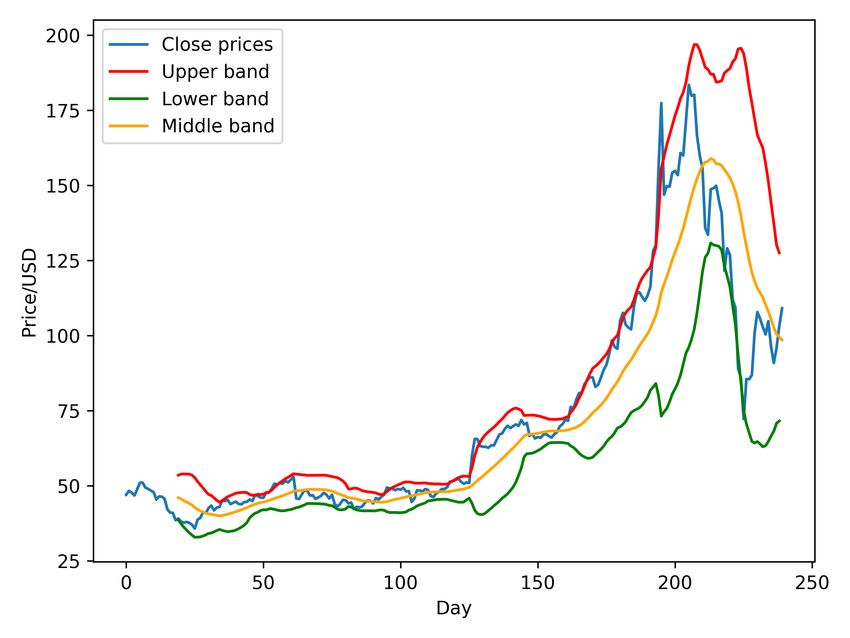
Typically, online brokers provide trading software for investors with some
technical indicators built-in to perform technical analysis. One of the foun-
dations to this is Candle Stick Chart, shown in figure 2.6.
The chart incorporates the information of stock prices and looks like a
candle, hence the name. To the left, we have a long/positive candle. The
filled part in green is called a body. The stick above and below is called
upper shadow and lower shadow. The lowest point and the highest point
indicate the lowest price and the highest price in a certain period. The top
and the bottom of the body indicates the close and open price in a certain
period [39, pp. 37].
To the right, there is a short/negative candle. It works similarly as a
positive candle, except for one difference: the top and the bottom of the
body indicates the open and close price in a certain period.
Now we move on to a 1-day tick chart. Figure 2.7 shows a stock price
movement within 39 trading days using 39 candle charts, each representing
1 trading day. There are also lines of different colours, such as green, blue,
purple, orange, cyan represents SMAs (simple moving averages, see chapter
2.5.1)
There are also weekly tick charts, monthly tick charts etc. for each secu-
19Figure 2.6: Candle Stick Chart
rity, given that the security has been listed long enough. For short-term
investment, trends are usually analysed using the 1-day tick chart.
There are many theories about drawing support lines and resistance lines,
as well as how to use them to predict trends. One way of doing that is shown
in the figure 2.7. It demonstrates a simple technical analysis. The local
maxima and minima are identified and they form a parallelogram which is
known as a trend channel [39, pp. 40]. It means that the stock will with
a high probability to move inside the channel. If the stock close price is
above the moving average (n) line then it is believed that the stock is going
up in periods of n and vice versa. Breaking through the resistance level
indicates that the stock is about to move upwards, and breaking out the
support level indicates the opposite. In this particular case, we can observe
that technical analysis successfully predicted stock movement intraday or
a few days ahead.
20Figure 2.7: Stock prices and technical indicators
2.5.1 Technical Indicators
Technical indicators, or technical oscillators, are mathematically calculated
signals that are used in technical analysis to predict future stock price
movements. Some widely used technical indicators are presented below.
2.5.2 Moving Averages
Simple Moving Average (SMA) is calculated by taking the average of a
series of values. Usually, the period n is one day and An is the closing price
of the day n. 5-day-average is written as SMA5 or SMA(5) [39, pp. 199].
A1 + A2 + ... + An
SM A =
n
2.5.3 Bollinger Bands
Bollinger Bands are a technical analysis tool for generating oversold or over-
bought signals. The middle band is also used to indicate a trend change.
The bands are computed as follows:
M B = SM A(n)
U B = SM A(T P, n) + m ∗ σ[T P, n]
LB = SM A(T P, n) − m ∗ σ[T P, n]
where:
SMA is simple moving average and n is usually 20 or 30,
21MB = Middle band,
UB = Upper band,
LB = Lower band,
TP (typical price) = (Highest price + Lowest price + Close price) / 3,
m is the number of standard deviations (usually 2),
σ[T P, n] is the standard deviation over last n periods of TP [39, pp. 209].
22Chapter 3
Methods
The chapter presents how the study was carried out. The selected methods
are motivated and discussed first, followed by a short explanation of them.
References are also provided for those who want to read further. The
workflow of this project is shown in 3.1 and will be explained in detail in
this chapter.
3.1 Choice of methods
In the literature study, two data collection methods were investigated. The
first alternative was to use a Twitter archive that was available for free on
the internet. However, it did not contain the complete set of tweets, nor
any relevant tweets about stocks. The second alternative was to purchase
a Twitter Developer subscription. Since the price was quite high and this
project was not sponsored by any company or organisation, the third option
was therefore used. Twitter has a free tier of Twitter developer which offers
access to historical tweets with limits. To comply with its user license
agreement, we decided to customise a Java program that collects tweets
with Twitter API.
In the data pre-processing part, Sul et al. [9] utilised one single attribute,
Twitter follower count to predict the emphabnormal return and promis-
ing results were found. Other attributes associated with tweets that were
dropped in their pre-processing step are therefore taken into account in this
study to answer the research question mentioned in chapter 1.2.
It is also known that financial instruments are widely used to predict stock
movements. As presented, previous studies have also implemented such and
23Figure 3.1: The workflow of this project
reached a not great result. These instruments can be easily implemented as
an extra column in the ML datasets. We believe that investors are affected
by psychology [2] hence we would like also to research if the addition of
financial instruments helps.
For evaluation, the objective is to find the best hypothesis function (the
neural network model) to predict future data. It is therefore often referred
to as the objective function or loss function. For regression problems,
typical loss functions are mean squared error, mean absolute error and
0/1 loss [37, pp. 711]. The mean squared error function has a smoother
curve. We believe that it will help to reach convergence better because
the learning step involving computing the gradient of the loss function. As
the gradient is constant for the mean absolute error, the loss value would
oscillate around the minimum point.
Other options include Mean Squared Percentage Error which is common
in trading because it is generally accepted that the percentage of change
matter much more than value changes [1], [4]. However, a comparison
between multiple data sets is not needed and the purpose of this study is
not to make money. Thus, the MSE loss function was chosen.
243.2 Development Environment
This thesis involves software development in Java and Machine Learning in
Python. For tweet collection, we used the library Twitter4J which provides
the search function and Twitter API authentication. We developed API
limit control and parsing the tweet on top of the library.
The data is preprocessed and cleaned in a Python program that was written
from scratch with the machine learning library Scikit-learn. The sentiment
scores are computed using the software VADER.
As for neural networks, we build our neural networks using the machine
learning library Keras. Development and experiments were carried out us-
ing PyCharm, a Python IDE (Integrated Development Environment). The
Keras library provides fundamental types of ”neurons” so that machine
learning engineers can focus on designing the architecture of the neural
network, tuning hyperparameters and understanding their data. The pro-
cessing of data as well as the technical analysis was written from scratch
using NumPy, which is a library providing numerical functions, like matrix
operations. Finally, data was visualised using the library Matplotlib.
3.3 Data Collection by Twitter API
Application Programming Interface (API) is easily explained as a tunnel
to make two computer programs talk to each other.
It is well known in data science that the quality of data is one of the most
important factors. We started with exploring data sets that suit our needs
and are available publicly, one of them being a website claiming that they
had the Twitter archive and they allow a full archive dump (rather than
just searching on the website). However, the archive covers only a small
fraction of the tweets and we could find only a few tweets per months that
were related to our topic.
Therefore, we decided to collect tweets using Twitter’s API, which is pro-
vided to developers who want to use Twitter data in their projects. Twitter
Inc. is a commercial company that offers free microblogging service. In re-
turn, Twitter may show ads and sell users data to cover the costs and make
a profit. Twitter has gained a huge market and many users use Twitter to
interact with each other, hence it becomes more and more popular for re-
searchers to acquire public opinions from it. To gain access to all historical
as well as real-time data, a premium subscription is required. Twitter has
25also restricted the usage with several tiers [40]. Since this project is not
sponsored by any company or organisation, the free subscription has been
used; It means that only the latest 7-day’s data is available and the total
GET requests that can be accepted by Twitter’s API server is limited to
180 requests every 15 minutes.
We developed a Java program to utilise Twitter API to collect the data.
We chose to study the stocks AMD (Advanced Micro Devices), Intel, Tesla
and Microsoft. The main reason is that these stocks are popular on Nasdaq,
and they are volatile. Furthermore, they are well-known so that people are
discussing on Twitter all the time. In the program, we use the functions
provided by Twitter API to search for tweets under certain constraints
including period, as well as observing search rate limit. As mentioned
before, the rate limit is 180 requests every 15 minutes. If the limit is
reached, we would get an error from Twitter API. Thus, we implemented a
rate monitor which pauses the searching progress when the limit is nearly
reached. A watchdog is also implemented so that the program will restart
if any error is encountered.
Table 3.1: Fields in the returned Tweet object used in this study
Field Description Use case
Keyword extraction and senti-
text The actual text of the Tweet.
ment analysis/classification.
How many times the tweet
Can be used to understand
favorite count has been favorited by other
how popular a Tweet is.
users.
The number of followers the To understand how influential
follower count
User who posted this Tweet. this user is.
The number of retweets of To understand how influential
retweet count
the original Tweet. this Tweet is.
Total number of Tweets within To understand how popular a
tweet count
a certain period. certain topic is.
If the account is verified by To verify the account is the
verified account
Twitter. ”real” account.
After the program sends a search request to Twitter through API, it will
catch the result returned from Twitter in a dictionary format. A dictionary
is a data structure that maps keys to values. Table 3.1 shows examples of
the fields (parameters associated with a tweet) in the API response. So that
the data can be processed later in a machine learning library, we parse the
Twitter object and stores the data in JavaScript Object Notation (JSON)
26format.
Inside the API response, the object tweet contains 15 to 30 tweets within
the period that the API query requested, and the object query provides
the information about whether all of the tweets are received or not. This
is essential because the program will request more tweets if the query is
not null but will stop requesting and stores all data into a JSON file if it
is null.
As mentioned in previous chapters, different Tweet may have a different im-
pact. For example, a verified account may have more authority to comment
on something, and their opinions may be more trusted by other people; Or
similarly, if an account is followed by many people, it may reach the wider
public and therefore impact the stock prices more. To limit the scope of
the project, We chose to extract 5 attributes associated with each Tweet:
the sentiment score, number of favourites, number of followers, number of
retweets and if an account is verified. The total number of tweets is also
taken into account. But since this value is not associated with the Tweet, it
is considered an extra feature in the training data set rather than another
attribute.
As for stock prices, Yahoo Finance provides free access to full historical
data, such as open, high, low and close prices as well as traded volume
(no intraday data). As shown in 2.5, there are 6 values for each day. The
variation of the price intraday may reflect the difference between how desire
investors are willing to buy and sell a stock. How this information is used
is explained in the next section.
3.4 Data Processing
3.4.1 Creating Training Examples
Before the collected data can be used to train the neural network model,
they usually need to be processed first. The reasons for doing so are many,
such as to remove noise or to make it easier for the neural network to be able
to extract patterns. For time series prediction problems, a filter is applied
to the data to create the training examples. Figure 3.2 demonstrates this
process with a filter length 5. Each colour corresponds to each unique
input data to the network. The first 5 elements are taken from the data
set. The first 4 elements will be the input (x) and the last element will be
the output (y). Next, the filter moves forward with step size 1 and another
training example is created. The filter will continue moving forward and
27this process is repeated until the filter reaches the end of the data set.
Figure 3.2: Creating training examples with filter length 5 and step size 1.
During training, the network will learn to use the input data to predict the
output data, which means, given a series of 4 consecutive values, the model
will output what value it believes the fifth value would be.
3.4.2 Adding Technical Indicators
The moving averages are calculated using the formel described in chapter
2.5.1 and are added to the data set. When calculating SMA5, 5 values
will be used to calculate the average value. The first row of the stock data
is 23 May 2019 and to calculate SMA5 for the same day, 4 previous days
stock value are needed. Thus, we have taken 20 extra days of stock data
to calculate Bollinger bands.
3.4.3 Sentiment Scores
To quantify the sentiment of tweets, a tool called VADER (Valence Aware
Dictionary and sEntiment Reasoner) is used. VADER is available as a
Python package, vaderSentiment. The Python class SentimentIntensity-
Analyzer inside this package takes text as input and output a score object.
We created an object of SentimentIntensityAnalyzer and called it with daily
tweets. Then we extracted the weighted compound score and saves it in a
CSV file. The score is finally added to the data set before training.
3.5 Neural Network Model
Earlier studies pointed out that the buyers and sellers use the historical
prices as well as the current trend to determine the price they are willing
28to pay and accept [41], [42]. Thus, the historical prices, as well as moving
averages, will affect future stock prices. It is therefore considered as a time
series forecasting problem, which makes it suitable for applying machine
learning.
To reach the goal of the project, a computational model that can compute
and combine both statistical patterns, time-oriented patterns and random
occurrence in data is necessary. The model should not overfit or under-fit,
and must be possible to combine two types of input training data; historical
stock- and twitter data, combined with additional features from Twitter
data.
Firstly, we collect historical stock price data from Yahoo Finance for up
to 10 years. Next, we use several mathematical models that are described
in Chapter 2.5.1, technical indicators. After this data processing step,
the training data for ML consist of 200 rows, which represent 100 trading
days. Each row contains market data, such as open price, close price,
volume, percentage, as well as sentiment scores of tweets the day before
the actual trade day. The sentiment score is calculated using VADER.
All these features are added as associations to stock price movement for a
single day, which provides now a complete data set. The data set is then
split into a training set, a verification set, as well as a test set, which are
used for machine learning [38].
Figure 3.3 shows the architecture of our machine learning model. First,
the input layer takes series of normalised stock prices, technical indicators
etc. as input. Then, the data is fed into the LSTM layers. The LSTM
nodes try to extract 100 features from them and output to the next layer
concatenate. This layer combines all features from input 1 and input 2 and
sends them to another LSTM layer. The output is sent to 2 fully connected
layers, i.e. the dense layers. Finally, the last dense layer will predict the
stock price. To prevent overfitting, dropout layers with a probability of
20% are added between the connected layers. In the neural network, we
use 10 neurons in the input layer, which represent the number of columns
in the data set. The hidden layers are specified in the figure. Then output
layer predicts the future price and the MSE is computed. For tuning the
hyperparameters, we experimented with different step-sizes, different num-
bers of hidden layers, neuron types, dropout rates and activation functions
to acquire an acceptable result.
29You can also read