Visual Transformer for Task-aware Active Learning - arXiv
←
→
Page content transcription
If your browser does not render page correctly, please read the page content below
Visual Transformer for Task-aware Active Learning

                                                          Razvan Caramalau1 , Binod Bhattarai1 and Tae-Kyun Kim1,2
                                                                       1
                                                                         Imperial College London, UK
                                                                            2
                                                                              KAIST, South Korea
                                                                  { r.caramalau18, b.bhattarai, tk.kim}@imperial.ac.uk
arXiv:2106.03801v1 [cs.CV] 7 Jun 2021

                                                                                      Abstract
                                                 Pool-based sampling in active learning (AL) represents a key framework for an-
                                                 notating informative data when dealing with deep learning models. In this paper,
                                                 we present a novel pipeline for pool-based Active Learning. Unlike most previ-
                                                 ous works, our method exploits accessible unlabelled examples during training
                                                 to estimate their co-relation with the labelled examples. Another contribution of
                                                 this paper is to adapt Visual Transformer as a sampler in the AL pipeline. Vi-
                                                 sual Transformer models non-local visual concept dependency between labelled
                                                 and unlabelled examples, which is crucial to identifying the influencing unla-
                                                 belled examples. Also, compared to existing methods where the learner and
                                                 the sampler are trained in a multi-stage manner, we propose to train them in a
                                                 task-aware jointly manner which enables transforming the latent space into two
                                                 separate tasks: one that classifies the labelled examples; the other that distin-
                                                 guishes the labelling direction. We evaluated our work on four different challeng-
                                                 ing benchmarks of classification and detection tasks viz. CIFAR10, CIFAR100,
                                                 FashionMNIST, RaFD, and Pascal VOC 2007. Our extensive empirical and qual-
                                                 itative evaluations demonstrate the superiority of our method compared to the
                                                 existing methods. Code available: https://github.com/razvancaramalau/
                                                 Visual-Transformer-for-Task-aware-Active-Learning

                                        1    Introduction
                                        In the recent success stories of Deep Learning in image classification [26, 19, 10] and object detection
                                        [28, 45, 16] the large-scale labelled data sets have been crucial. Data annotation is a time-consuming
                                        task, needs experts and is also expensive. Active Learning [24, 29, 30, 5, 4] is getting popular to
                                        select a subset of discriminative examples incrementally to learn the model for downstream tasks. In
                                        the AL frameworks usually, a learner, a sampler, and an annotator complete a loop and repeat the
                                        cycle. In brief, a learner minimizes the objective of the downstream task and the sampler selects the
                                        representative unlabelled examples given a fixed annotation budget. And, an annotator queries the
                                        labels of the unlabelled data recommended by the sampler. Based on the category of the employed
                                        sampler, the whole paradigm of AL can be broadly dissected into uncertainty based [21, 14, 23],
                                        geometric based [39, 31], model based [42, 35, 1, 15], and so on.
                                        In this paper, we focus on model based [35, 5, 42] active learning pipelines for pool-based sampling.
                                        The importance of this type of pipeline is growing and getting more relevant than ever before due to
                                        the increasing use of deep learning algorithms. In this scenario, given a large volume of unlabelled
                                        data, an initial model is trained on a small subset of randomly annotated examples. In the later stages,
                                        the samples are annotated in the guidance of the model trained in the previous stage. The fate of
                                        this method category is determined by the performance of initial model which is commonly known
                                        as cold-start problem [15]. To tackle such a problem and improve the performance of the model in
                                        its early stage, training the model in a semi-supervised fashion is slowly getting into attention [15].
                                        Exploiting unlabelled data along with the labelled data in joint or a multi-task setup improves the

                                        Preprint. Under review.
generalization of the model [7]. However, the previous work minimizes the loss functions such as
consistency loss [15] which is indirect to the downstream task i.e. class category loss. Also, these
methods rely only on exploiting unlabelled data to improve the performance of the model. Unlike
these methods, our approach tackles this problem from both aspects i.e. making use of unlabelled
data as well as engineering the model architecture. To this end, we adapted Visual Transformer [40]
in the pipeline with the learner and exploited the unlabelled data for better generalisation. Finally, we
train the model in a joint-learning framework by minimizing a labelled vs unlabelled discriminator
(sampler) as well as the downstream task-aware loss.
Visual Transformers (VT) [40] are attaining state-of-the-art results on various tasks such as image
classification [10, 40], detection [6], and so on. To the best of our knowledge, this is the first work
adapting VT for active learning framework. Figure 1 demonstrates the pipeline of the proposed
method. A batch of both the unlabelled and labelled examples are passed through few convolutional
layers sequentially. The output batch from these layers are fed into the VT layers at once. CNN layers
are myopic in nature by extracting the statistics of local information as image features. Uncertainty
on such feature space helps us to select images with variations on blurriness, contrasts, textures etc.
However, a non-local interaction between the unlabelled and labelled examples is essential to identify
the complimentary examples to query their labels. To this end, we propose to integrate VT in between
CNN layers and the output layer. Previous works on VT for computer vision [10] divided the images
by a regular grid to extract local patches and fed them to VT to extract the non-local interactions
between parts of an image. As our task is to identify the most discriminative images, hence, we
consider each level representation of both labelled and unlabelled examples as an input channel to this
module. Thus, VT extracts non-local interactions between the labelled-unlabelled examples while
uncertainty on such feature space allows us to select the images which are sufficiently different on a
visual concept. The output of the VT is feed to output which is bifurcated into labelled vs unlabelled
discriminator and task-specific auxiliary classifier. Uncertainties on feature space to minimizing
these two losses help us to find the unlabelled examples which are sufficiently different to labelled
examples and relevant to the downstream task. This address the problem of earlier methods [31]
selecting examples from high-density regions irrespective of the decision boundary.
We summarise the contributions of this paper in the following bullet points:

       • We propose a novel task-aware joint-learning framework for active learning.
       • We adapted Visual Transformer for the first time in the pipeline of active learning.
       • We evaluated our methods for sub-sampling real and synthetic examples for four different
         image classification and one object detection benchmarks.
       • We outperformed existing methods by a large margin and attain a new state-of-the-art
         performance.

2   Related Works
The current taxonomy of active learning is founded on the extensive survey of Settles [32]. This
gathers all the classical approaches together with the three scenarios of active learning. Most deep
learning works, including ours, rely on the pool-based scenario. Depending on the mechanisms used
for sampling or deriving heuristics of the unlabelled data, we can categorise methods as uncertainty-
aware, geometric representation and model-based. The first category has been initially applied with
the Monte Carlo (MC) Dropout approximation for deep Bayesian models of Gal et al.[13]. Thus, the
selection in the active learning study [14] is inspired from classical approaches as maximum entropy
[33] or BALD [21]. Another approach of gathering the uncertainty from models is by querying a
committee machine [32]. A recent work that expanded to deep learning this classic principle has
been presented by Beluch et al.[2]. This method overcame in performance the works centred on the
MC Dropout mechanism. However, with the complexity increase of current deep learning models,
both iterative approaches have proven to be hardly applicable.
On this concern, the second category tackles this issue by evaluating geometrically the representations
of the downstream task. We acknowledge Senner and Savarese [31] as the most representative work
with the CoreSet algorithm. Their methodology evaluates a global fixed radius to cover the feature
space by selecting a subset of unlabelled. This has been succeeded by other learners of [24, 36, 18].
We include this competitive baseline for comparison in our experiment section.

                                                   2
Offline selection
                                                                                             TJLS
                                          Annotation
    Labelled data                          System
                                                                                        Active Learning

                                                 Visual Transformer                  Sampler       BCE Loss

                        CNN                              Batch
                       Feature                                             Feed                    Joint learning (3)
                                                          Self-
                      Extractor                                           Forward
                                                        Attention

                                                           (1)                 (2)
                                                                                       Feed
                                                                                     Forward        CE Loss
                                        Passing both labelled and unlabelled
    Unlabelled data                              Back-propagation
                                               Passing just labelled

Figure 1: This diagram depicts the proposed pipeline. We pass both the labelled and unlabelled
examples through the same CNN and extract the visual features of each image encoded within the
batch. These representations are fed to the Visual Transformer. Its outputs are passed to the bifurcated
branches to minimize both the learner’s (class cross-entropy ) and the sampler’s objectives (binary
cross-entropy).

The third category, and the most recent one, deploys dedicated learning models, also referred to as
samplers, for querying new data. The first proposed module, Learning Loss [42], tracks uncertainty
by training end-to-end and estimating the predictive loss of the unlabelled. The modular aspect of this
category permits deploying the samplers to diverse applications. Our method inherits this advantage.
Sinha et al.[35] defined the sampler training framework VAAL separately where a variational auto-
encoder (VAE) maps all the available data in a latent space. The selection principle is based on the
adversarially trained discriminator between labelled and unlabelled. The fallback of this method,
lack of task-awareness, has been addressed in [44, 1, 4]. Hence, Agarwal et al.[1] proposes CDAL
that combines the sampler with the contextual diversity while enlarging the receptive feature domain.
Following similar trends, Caramalau et al.[4] deploys Graph Convolutional Networks (GCNs) for
feature propagation between labelled and unlabelled images. These works are close to ours and are
evaluated in the experiment section.
Because our proposed AL framework combines the semi-supervised learning (SSL) strategy with a
visual transformer, we further investigate related literature. SSL and AL have been recently considered
for deep learning in a few works [15, 31, 11, 27]. The first attempt is noted in CoreSet [31] during
AL cycles. A more elaborated method CSAL analyses the consistency loss of unlabelled data when
trained end-to-end. Thus, it achieves state-of-the-art on the image classification datasets. Furthermore,
we outperform this baseline in our analysis under their experiment settings. On the other end, the
visual transformer has been initially designed for vision applications by Dosovitskiy et al.[10]. They
considered the natural language processing BERT [9] approach on patches of the images to learn the
non-local representations. Following this work, transformers have successfully replaced convolutional
layers in [40] while boosting the accuracy under a similar number of parameters. Our methodology is
supported by the insights from this research.

3    Method

In this Section, we start with the formal definition of pool-based Active Learning in general followed
by our contributions on introducing VT in the pipeline and the task-aware joint-learning objective.
Given a large pool of unlabelled data xU ∈ Upool , the pipeline begins with a cold-start training of the
model by randomly selecting a small subset and labelling an initial set xL0 , yL 0 ∈ L0 ⊂ Upool . The
performance of the initial model is crucial for the end outcome of the framework [15] for model-based
active learning. Our contribution lies in addressing this problem which is also commonly known
as cold-start problem. To this end, we took two approaches: jointly learning the parameters of the
learner and sampler utilising the accessible unlabelled examples and adapting the Visual Transformer
as a bottleneck of the pipeline. If b is the budget to sample unlabelled examples over multiple
selection stages, the main objective of the pool-based AL scenario is to obtain fast generalisation of

                                                          3
the learner with the least number of labelled subsets n in order to keep minimum samples. ∀i ∈ n,
Li = (xLi , yL i ) ⊂ Upool represents the annotated examples in every ith subset.
Figure 1 outlines the proposed pipeline. From the Figure, we can see that both the labelled and
unlabelled examples are fed to the image feature extractor, f . For most vision applications, the
backbone of the learner is a feature extractor commonly formed of CNNs such as ResNet [19]
and VGG architectures [34]. From the initial labelled set, xL0 , yL 0 ∈ L0 and U0 ∈ Upool \ L0 ,
unlabelled examples, we infer them to the feature extractors. In our case, we take an equal number
of labelled and unlabelled examples to balance the number of training examples. In a batch of
B examples, we choose both unlabelled and labelled examples and feed them into f (θf ) where
f : RB×W H×C → RB×wh×|F | . Here, W, H are height and width of the images, C is channels of
input images, w, h are width and height of channels from the last convolutional layer, |F | is the total
number of filters on the last convolutional layer of feature extractor. Earlier methods [5, 42] feed
the output of the convolutional layers to the output layers to minimize the loss. Instead, we feed the
output of these layers to the Visual Transformer before feeding to the output layers. CNN layers
handle only local dependencies, but non-local dependencies between the labelled and unlabelled
examples are essential to select the complementary unlabelled examples. Visual Transformer has
been quite successful in modelling non-local dependencies. UncertainGCN [5] uses GCN to handle
long-range dependencies in Active Learning. A comparative study on GCN and self attention [40]
has been shown that the self-attention aggregation function retains better the diverse concepts than
the GCN.
Visual Transformer. [10] is the first work to apply Visual Transformer successfully for image
classification. In this work, each image is divided by regular grids into patches and each of the
patches is considered input tokens to the transformer. Another following work [40] compressed the
features of CNN backbones to visual tokens while the transformer acted as the final convolutional
layer. Inspired by these works, we plugged a visual transformer as a neck between the feature
extractor and the output layer. In our case, the inputs to the transformer are batches of feature maps
that we obtained from the feature extractors as f : RB×W H×C → RB×wh×|F | .
Different from [10, 40], we foresee the AL framework to be least intrusive to the learner’s architecture.
This allows the methodology to be plugged into various designs and applications. We, therefore, do
not further post-process the output of CNN feature extractor. Similarly to GCNs [22], we want to
explore the relationships between the nodes of the graph. However, given our input f (x; θf ) (θf are
the parameters of the feature extractor), we propose to deploy the transformer blocks within the batch
B. Consequently, all the channels of the feature maps from each batch are considered as tokens to
VT. Although in the standard architecture [38], the inputs to the transformer are positional encoded,
this does not apply in our scenario where the order of the images is irrelevant. As mentioned in the
Introduction, our objective is to extract non-local relationships between the images not within the
image. To simplify furthermore the transformer’s architecture, we exclude the decoder part as the
target domain is absent in our case.
From the seminal work on self-attention [38], the main building blocks of the transformer’s encoder
are a batch self-attention block and a point-wise feed-forward network with residuals and layer
normalisation. For the self-attention, we transpose to the batch and concatenate the feature maps
so that fT (x; θf ) ∈ Rwh|F |×B . The key, query and value matrices (WKatt , WQatt , WVatt ) are
packed together to model the interactions between the features. This also favours inner-domain
relationships as batch normalisation is commonly used in CNNs for regularisation. The operations of
the batch self-attention are summarised as follows:

                         softmax((fT (x; θf )WKatt )(fT (x; θf )WQatt )T )
  Tatt = fT (x; θf ) +                      p                              (fT (x; θf )WVatt ),      (1)
                                              dimKatt

where Tatt and softmax are the output of the batch self-attention layer and its activation function.
While keeping the dynamics within the batch, we pass Tatt through the point-wise feed-forward
network. We define Tout (fT ; θg ) the output of this block, with θg as all VT parameters. The
following equation underlines its processes:

                                 Tout = Tatt + σ(Tatt Wh1 )Wh2 ,                                     (2)

                                                   4
where Wh are the weights from the feed-forward network and σ represents the sigmoid activation
function.
Task-Aware Joint-Learning. Recently, the state-of-the-art for deep active learning has been gained
by model-based methods like Learning Loss[42], VAAL[35], CDAL[1] and UncertainGCN[5]. These
fundamentally comprise dedicated trainable models to sample unlabelled data. Apart from Learning
Loss, the downfall of these methods is the sub-optimal multi-stage training processes. Also, in limited
budget scenarios, the risk of over-fitting appears from the initial cold-start sampling. Unlike the
approaches of these methods, we proposed to optimise the parameters jointly. Also, customize the
objective depending upon the downstream tasks. In our case, we have considered image classification
and object detection. But, our method can be easily extended to other tasks.
The representations of the labelled examples and unlabelled examples from the transformer are fed
into the bifurcated branch of the network. One of them minimizes the binary cross-entropy loss to
distinguish labelled examples from unlabelled examples. Another branch minimizes the task-specific
loss. For the classification task, we minimize class categorical loss. Similarly, for object detection,
we minimize the combination of confidence and localisation loss as stated in [28]. Thus the overall
objective of the network when the downstream task is classification task is as shown in the Equation 4.
In the same manner, the overall objective becomes as stated in Equation 3 when the downstream task
is object detection. In the Equations, λ1 , λ2 are the weighting factors corresponding to each task. θ1
and θ2 are the learnable parameters of the main task and the sampler branch, respectively.
To learn them, we apply gradient back-propagation. We alternate the gradient between the sampler
and the task branch for every batch of data as shown by the backward head arrow in Figure 1. This
adds an inductive bias while avoiding over-fitting the data or the random noise. An elaborated
deduction was presented by Goyal et al.in [17].

              LJL = λ1 LCE (xL0 , yL 0 ; [θ1 , θg , θf ]) + λ2 LBCE (xL0 , 1; [θ2 , θg , θf ]),     (3)
             LJL = λ1 LSSD (xL0 , yL 0 ; [θ1 , θg , θf ]) + λ2 LBCE (xL0 , 1; [θ2 , θg , θf ]),     (4)
Sampling the unlabelled data. To recap, the proposed AL framework trains jointly both learner and
sampler. As a bottleneck between feature extractor and output layers, we add a visual transformer
between the feature extractor and the two task branches. Combining the unlabelled and labelled data
helps in preserving the most meaningful features during the learning stage. Moreover, the transformer
will be exposed also to the unlabelled data dependencies. This happens as the task of the sampler
is to classify the labelled from the unlabelled. The two are categorised as 1 or 0, respectively. If
the unlabelled examples xU0 ∈ U0 are easily differentiated by the sampler, we want to target for
selection the most uncertain xU ∈ Upool .
Similarly, it has been done in an adversarial manner by VAAL [35], although their AL framework is
not linked with the main task. Therefore, we derive our selection principle from UncertainGCN[5].
Given a budget of b points, we infer the entire unlabelled pool and select the samples with the
lowest posterior probability of the discriminator branch. We notate PS as the confidence score of the
posterior. Considering the first selection stage, we can evaluate the new labelled set L1 with:

                                   L1 = L0 ∪ arg max PS (xU ; θ2 ).                                 (5)
                                                  i=1···b

We compute the arg max because the highest confidence score for the unlabelled is when PS (xU ; θ2 )
is closer to 0. This selection process along with re-training is repeated until the targeted performance
of the downstream task is reached.
For convenience, we denote the proposed AL framework as TJLS( Transformer with Joint-Learning
Sampler). In the next part, we thoroughly quantify the stated method and motivations. Furthermore,
to observe the impact of the transformer bottleneck, we also investigate the pipeline JLS without it.

4   Experiments
Here we present both the quantitative (including ablation studies) and qualitative evaluations in a
detailed manner. We employed our method TJLS (visual transformer in the joint-learning sampler)
for two different tasks: image classification and objection.

                                                     5
Baselines. We choose state-of-the arts from different categories like uncertainty-based (MC Dropout
[13], DBAL [14]), geometric (CoreSet [31]) and the most recent model-based (Learning Loss [42],
VAAL[35], CDAL[1], CSAL[15]).
The standard practice to acquire datasets is through random sampling from the uniform distribution.
This does not require any active learning mechanism for selection. The first methods to explore
the uncertainties in deep learning models have been MC Dropout and, its extension, DBAL. Both
approximate the learner in a Bayesian fashion. The two uncertainty-based methods differ by their
selection criteria. MC Dropout relies on maximum entropy, while DBAL maximises information
with BALD [21]. From a geometric perspective, the most successful work, CoreSet [31], estimates
risk minimisation between the labelled set and a core points of unlabelled. Fundamentally, a k-centre
Greedy [39] algorithm measures the distances between labelled and unlabelled learner’s features.
As our method falls in the third category, model-based, we assess four recent state-of-the-art: Learning
Loss [42], VAAL[35], CDAL[1], CSAL[15]. The first work to introduce learnable parameters for
sampling is Learning Loss. Similarly, to our work, they train end-to-end the learner with the sampler,
but the extra module predicts the downstream task loss. A more complex sampler has been proposed
by VAAL where a variational auto-encoder is trained in an adversarial manner with both labelled
and unlabelled data. The selection principle is close to ours by picking the hardly discriminated
samples. However, the sampler is not task-aware with the main objective. On the other hand, CDAL
provides a reinforcement learning module for a Bi-LSTM [20] that captures the contextual diversity
of the learner. Their selection criteria keeps the unlabelled batches with the highest reward. The last
baseline that we tackle in our experiments is CSAL. This method also optimizes the task model with
unlabelled samples as in JLS. The main difference to ours consists in using augmented unlabelled
data to compute a consistency loss that does not overlap with the end task.

4.1   Image Classification

Datasets and Implementation Details. For image classification, we took three well known data sets:
CIFAR-10, CIFAR-100 [25] and FashionMNIST[41]. The training set of each of the dataset makes
Upool . CIFAR-10 and CIFAR-100 consists of RGB images whereas FashionMNIST is grey-scale.
From an architectural perspective, we swap the main deep CNN model between VGG-16 [34] and
ResNet-18 [19]. These learners are combined with the visual transformer and the sampler of our
method TJDS. We set the hidden dimension of the transformer block for both self-attention and
feed-forward module to 128. The label discriminator part of the sampler is composed of two layers.
The hidden units of both of them are 512. We fixed these values for our pipeline for these experiments.
Part of the hyper-parameter tuning behind this configuration is discussed later in this section. In
Equation 4, we weight the impact of the two losses by λ1 and λ2 . From cross-validation, we notice
that setting the weight of the sampler (λ1 ) to 50% of the auxiliary loss (λ2 ) brings more stability in
joint-learning. However, λ1 is set to 1 when labelled images are inferred through the downstream
task. During training, we fix the batch size to 128 for all the methods. We optimize the gradient of
the joint-learning with SGD by setting a learning rate of 0.01, a weight decay of 5e-4, and epochs to
200. To measure the performance of the AL framework, we evaluate the mean accuracy over 5 trials
for 7 selection stages.
Quantitative analysis. We deploy VGG-16 for the CIFAR-10 and CIFAR-100 experiments. We
start with an initial labelled set xL0 with 10% of the original training set. For the selection phase,
we allocate a budget b of 5% every time identical to that of VAAL[35] or CDAL[1]. Our TJLS or
JLS algorithm requires a subset xU0 of unlabelled examples to train the sampler branch. In these
benchmarks, we vary this set equal to the percentage of labelled. Following this, the sampler is not
biased towards any group.
The Figures from 2 demonstrate quantitatively the top performance that our two versions (JLS and
TJLS) achieve on CIFAR-10 (left) and CIFAR-100 (middle). The important thing to notice is that
the proposed AL outperforms the baselines by a large margin from the very early stage. Also, the
performance gain over the baselines is sustained even in the later stages. This highlights the need
and importance of addressing cold-start problem in model-based AL frameworks. Among the two
variants of our model, TJLS and JLS, the former is more effective than the latter one. This highlights
the key role played by the transformer in non-local dependency modelling. We observe a similar trend
on FashionMNIST (See Figure 2 (right)) which is another popular grey-scale image classification
benchmark.

                                                   6
Testing accuracy on CIFAR-10 Testing accuracy on CIFAR-100 Testing accuracy on FashionMNIST
85
90 65
60 80
Accuracy (mean of 5 trials)
Accuracy (mean of 5 trials)
Accuracy (mean of 5 trials)
85
55
80 75
50
75 45 70
70 Random Learning Loss 40 Random Learning Loss 65
MC Dropout CDAL MC Dropout CDAL Random CDAL
DBAL JLS 35 DBAL JLS CoreSet JLS
65
CoreSet TJLS CoreSet TJLS 60 VAAL TJLS
VAAL 30 VAAL Learning Loss
60
10 15 20 25 30 35 40 10 15 20 25 30 35 40 100 200 300 400 500 600 700
Percentage [%] of labelled samples Percentage [%] of labelled samples Number of labelled samples
Figure 2: Quantitative evaluation on the CIFAR-10 left, CIFAR-100 middle sets with VGG-16 and
FashionMNIST (right) with ResNet-18(right) [Zoom in for better view]
Comparison with SSL 25% 30% 35% 40%
CSAL [28] 67.93 68.97 69.8 70.51
JLS 70.2 71.3 72.18 71.56
TJLS 70.22 71.62 72.45 72.14
Table 1: Comparison with the semi-supervised CSAL method on CIFAR-100 with a Wide ResNet-28
learner
In addition to previous figures, we compare the contemporary state-of-the-art SSL method CSAL [15].
We explicitly present in Table 4.1 the quantitative results under the configuration of their work where
a Wide ResNet-28 [43] backbone is plugged. Beginning the AL selection at 25% of CIFAR-100 data,
our frameworks outperform by at least 2% in testing accuracy over four stages without adding any
augmented data. The results have been averaged from 3 trials.
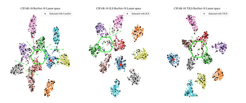
Intrinsic discussions. For a better understanding of our AL framework, we analyse the behaviour and
visualise the latent features of the learner at the first selection stage through t-SNE[37] distributions.
Therefore, we run a fixed labelled set experiment on CIFAR-10 to represent both labelled and
unlabelled after the second cycle of active learning. We deploy the ResNet-18 backbone for both JLS
and TJLS. However, we also include the latent space evaluation for the learner without joint-learning.
In this case, we apply CoreSet during the AL selection so that we can qualitatively compare it with
our approach.
Figure 3 displays the three t-SNE latent spaces from the specified models: ResNet-18, JLS ResNet-18
and TJLS ResNet-18. All the images come from the available unlabelled pool. However, we already
assign the 10 labels to visualise better the clusters. On this note, we also sub-sample both selected
(marked with crosses) and unlabelled sets. The green hexagons added to the Figure mark the cluttered
areas where some clusters are adjacent. The dotted lines also delimit presumed boundaries between
classes. With these highlights, we can observe that JLS and TJLS provide more robust representations
than the naive baseline. Moreover, in the cluttered areas, the sampler’s uncertainty principle draws
more samples than CoreSet. This will further boost the accuracy in the next training cycle.
Ablation studies. Although the main methodology, TJLS, relies on the visual transformer, throughout
the paper, we also test the variant without it, JLS. The combined analysis leverages our motivation
Figure 3: Intrinsic analysis of the latent space and the active learning selection [Zoom in for view]
7
Selection criteria for TJLS    10%     15%     20%     25%     30%     35%     40%
         TJLS + Random sampling         71.1    70.44    68.1   66.47   62.41   62.36   62.15
         TJLS + CoreSet [18]              -     72.35   73.55    74.3   74.5     74.6   75.3
         TJLS Uncertainty sampling        -     73.72    74.3    74.8   75.3     75.6   75.67
Table 2: Evaluation of different selection functions for TJLS on CIFAR-100 with ResNet-18 backbone

                  Ablation study        10%     15%     20%     25%     30%      35%    40%
                       JLS                43     50      55.7   59.1     63       65    67.1
                    JLS + GCN            45.6   54.23    59.1   61.9    64.51    67.4   69.6
             JLS + Transformer (TJLS)   48.97   56.67   61.89   65.54   67.77    69.9   71.7
Table 3: Ablation study - CIFAR-100 testing performance of the joint-learning sampling scheme
(JLS), with GCN bottleneck and with TJLS (Learner VGG-16)

from the methodology. Furthermore, we re-iterate the comparison between the two and we explore
the possibility of replacing the transformer with a GCN. In Table 4.1, we present the results of the
three joint-learning architectures. Compared to Figure 2 results, we follow the same settings and CNN
backbone but we increase the number of unlabelled examples used for training by 50%. The GCN is
replacing the transformer bottleneck in the second row of Table 4.1. Its design is inspired from [22]
where the nodes of the graph change with input batch. Similarly to the transformer bottleneck, we
want to model the higher order of representation that CNN lacks. The results in Table 4.1 confirm the
TJLS proposal by achieving the best accuracy with every labelled subset. The selection criteria of
uncertainty sampling has been kept for all three variants.

   TJLS                                               Transformer
               10%      20%     30%     40%
 batch (B)                                            parameters         10%     20%     30%      40%
     16         57.5    66.2   69.68     72.1    depth heads units
     32         64.4   71.42    73.8     75.3      1       1      512   43.05    53.9    62.06   65.59
     64        70.12    74.3    75.4    75.74      1       2      128   44.41   56.05    61.83   66.19
    128         71.1    74.3    75.3    75.67      2       1      128   42.46   57.04    63.45   66.36
Table 4: Hyper-parameter study. (Left) ResNet-18 backbone, batch size variation. (Right) VGG-16
backbone, Transformer architectural configuration. Dataset: CIFAR-100, [mean of 3 trials], % of
labelled data

Sampler hyper-parameter study. The sampler of our pipeline TJLS consists of two building blocks,
the visual transformer and a fully-connected discriminator. We empirically evaluated both models by
grid-searching the optimal architectures. However, in the discriminator case, we maintain a similar
structure to the downstream task branch so that features fall under the same domain. Thus, the focus
of the parameter tuning is mainly on the transformer block. Table 4.1 presents the most meaningful
results where the batch size is varied (on the left) together with depth, heads and hidden units. With
the increase of the batch input size, Table 4.1 (left), we observe that the feature’s relationships are
better explored. This justifies the pre-defined settings. On the right side, when changing the hidden
units to 512, the gains of TJLS drop at the first selection stages. Despite this, we acknowledge that by
increasing the depth or the number of heads [38], our pipeline can achieve robust performance with
different amounts of data.

4.2   Object Detection

Our method is generic and can be extended to other tasks simply customizing the task-specific
auxiliary loss in the pipeline. Hence, we replace the categorical cross-entropy loss with SSD [28]
loss and employed it on the object detection benchmark.
Dataset and Implementation Details. The first work to tackle active learning for object detection is
Learning Loss [42]. In this regard, we follow the same dataset, learner and parameter settings. Briefly,
the unlabelled pool consists in 16551 images from PASCAL VOC 2007 and 2012 [12]. Compared to
image classification, we start a first randomly labelled set of 1000 and we increase the budget with the
same rate. However, we apply the AL selection process within 10 stages. As in [42, 1], the learner’s
architecture is SSD[28] with a VGG-16[34] backbone. The visual transformer bottleneck from our
joint-learning selection is positioned only on the confidence head of the SSD network. For every AL
stage evaluation, we compute the mAP metric of PASCAL VOC 2007 testing set while averaging

                                                    8
Testing accuracy on Pascal VOC                                                                              Sub-sampling of augmented data on RaFD
                                                                                                                                                     95.0
                               75

                                                                                                                  Test accuracy (mean of 5 trials)
                                                                                                                                                     92.5

      mAP (mean of 5 trials)
                               70                                                                                                                    90.0

                                                                                                                                                     87.5
                               65
                                                                                                                                                     85.0
                                                                                              Random
                               60                                                             Entropy                                                82.5
                                                                                              CoreSet
                                                                                              Learning Loss
                                                                                                                                                     80.0
                               55                                                             CDAL                                                                                                       Random
                                                                                              JLS                                                                                                        UncertainGCN
                                                                                              TJLS                                                   77.5                                                TJLS
                                    1000   2000   3000     4000   5000   6000   7000   8000   9000   10000                                                  0      1000          2000         3000              4000
                                                         Number of annotated samples                                                                                       Synthetic images

Figure 4: Quantitative evaluation on Pascal VOC 0712 dataset with SSD (left) and StarGAN synthetic
data set (right) [Zoom in for better view]

over 5 trials.
Quantitative analysis. Figure 4 (left) illustrates the comparisons of the proposed baselines on the
object detection experiment. The trends of JLS and TJLS behave similarly to the image classification
point. They show a great level of generalisation from the cold-start at 62.5% mAP while having
a 10% performance gain over the other baselines. The uncertainty-based selection is appropriate
with the learner’s representation through all the 10 selection stages. Therefore, both JLS and TJLS
saturate with top performance from the 7th cycle at over 76% mAP. Our method outperforms the
previous state-of-the-art Learning Loss and CDAL. However, between the two proposed variants,
TJLS provides non-local interactions within the batch. This advantage is reflected quantitatively
against JLS in this task as well.

4.3                            Subsampling synthetic data

Sub-sampling synthetic data to augment the real data is an active research [5, 3]. Following the
experimental setup of Caramalau et al. [5] for sub-setting synthetic data, we employed our pipeline to
select the face expression synthetic data generated by StarGAN [8]. The selected synthetic data were
augmented with the RaFD1 real training data to train to a model for face expression classification
task. Figure 4 (right) shows the performance comparison. Our method surpasses the performance of
existing arts by a large margin.

5                Conclusions and Limitations
In this paper, we present a novel model-based active learning. Our contributions are the adaptation
of Visual Transformer to address non-local dependencies between all the examples and exploitation
of the unlabelled data by jointly minimizing the task-aware objective. Our extensive empirical
and qualitative analysis on multiple benchmarks demonstrate the efficacy of the proposed method
compared to the existing method. The main fallback to address in the proposed method is scalability.
We acknowledge that introducing the visual transformer in TJLS increases the number of target model
parameters. Despite this, our proposal relies on the current and future technological advancements
where there has already been continuous growth. Another caveat consists of the restriction of the
batch self-attention block. Some architectures might require smaller batch sizes where the benefits of
TJLS can be affected. From recent works [40, 10], it has been shown that visual transformers demand
a big corpus of data. However, by including the unlabelled examples as part of the TJLS training, we
satisfy this requirement. In future work, we would like to explore our method to efficiently handle
high-resolution data.
 Broader impact: Active learning is a dynamic and important research topic. Our contribution lies
in the methodology of active learning. We believe that the research proposed in this paper can be
further applied where large-scale data and annotation presents an issue. Thus, this might serve to
fields like medical imaging, robotics and many other. Moreover, integrating TJLS as a sampling
framework would yield greater performance in a limited labelled data scenario. Our method opens a
new direction in the active learning research being sustained by state-of-the-art results.

      1
           http://www.socsci.ru.nl:8180/RaFD2/RaFD

                                                                                                              9
References
 [1] Sharat Agarwal, Himanshu Arora, Saket Anand, and Chetan Arora. Contextual diversity for
     active learning. In ECCV, 2020.
 [2] William H Beluch Bcai, Andreas Nürnberger, and Jan M Köhler Bcai. The power of ensembles
     for active learning in image classification. In CVPR, 2018.
 [3] Binod Bhattarai, Seungryul Baek, Rumeysa Bodur, and Tae-Kyun Kim. Sampling strategies for
     gan synthetic data. In ICASSP, 2020.
 [4] Razvan Caramalau, Binod Bhattarai, and Tae-Kyun Kim. Active learning for bayesian 3d hand
     pose estimation. In WACV, 2021.
 [5] Razvan Caramalau, Binod Bhattarai, and Tae-Kyun Kim. Sequential graph convolutional
     network for active learning. In CVPR, 2021.
 [6] Nicolas Carion, Francisco Massa, Gabriel Synnaeve, Nicolas Usunier, Alexander Kirillov, and
     Sergey Zagoruyko. End-to-end object detection with transformers. In ECCV, 2020.
 [7] Rich Caruana. Multitask learning. Machine learning, 28(1):41–75, 1997.
 [8] Yunjey Choi, Minje Choi, Munyoung Kim, Jung-Woo Ha, Sunghun Kim, and Jaegul Choo.
     Stargan: Unified generative adversarial networks for multi-domain image-to-image translation.
     In CVPR, 2018.
 [9] Jacob Devlin, Ming-Wei Chang, Kenton Lee, and Kristina Toutanova. BERT: Pre-training
     of deep bidirectional transformers for language understanding. In Proceedings of the 2019
     Conference of the North American Chapter of the Association for Computational Linguistics:
     Human Language Technologies, Volume 1 (Long and Short Papers), June 2019.
[10] Alexey Dosovitskiy, Lucas Beyer, Alexander Kolesnikov, Dirk Weissenborn, Xiaohua Zhai,
     Thomas Unterthiner, Mostafa Dehghani, Matthias Minderer, Georg Heigold, Sylvain Gelly,
     Jakob Uszkoreit, and Neil Houlsby. An image is worth 16x16 words: Transformers for image
     recognition at scale, 2020.
[11] Thomas Drugman, Janne Pylkkönen, and Reinhard Kneser. Active and semi-supervised learning
     in asr: Benefits on the acoustic and language models. In INTERSPEECH, 2016.
[12] Mark Everingham, Luc Gool, Christopher K. Williams, John Winn, and Andrew Zisserman.
     The pascal visual object classes (voc) challenge. International Journal of Computer Vision,
     2010.
[13] Yarin Gal and Zoubin Ghahramani. Dropout as a Bayesian Approximation: Representing Model
     Uncertainty in Deep Learning. In ICML, 2016.
[14] Yarin Gal, Riashat Islam, and Zoubin Ghahramani. Deep Bayesian Active Learning with Image
     Data. In ICML, 2017.
[15] Mingfei Gao, Zizhao Zhang, Guo Yu, Sercan Arik, Larry Davis, and Tomas Pfister. Consistency-
     based semi-supervised active learning: Towards minimizing labeling cost. In ECCV, pages
     510–526, 2020.
[16] Golnaz Ghiasi, Yin Cui, Aravind Srinivas, Rui Qian, Tsung-Yi Lin, Ekin D. Cubuk, Quoc V.
     Le, and Barret Zoph. Simple Copy-Paste is a Strong Data Augmentation Method for Instance
     Segmentation. arXiv e-prints, 2020.
[17] Anirudh Goyal and Yoshua Bengio. Inductive Biases for Deep Learning of Higher-Level
     Cognition. arXiv e-prints, 2020.
[18] Sariel Har-Peled and Akash Kushal. Smaller coresets for k-median and k-means clustering. In
     SCG, 2005.
[19] Kaiming He, Xiangyu Zhang, Shaoqing Ren, and Jian Sun. Deep residual learning for image
     recognition. In CVPR, 2016.
[20] Sepp Hochreiter and Jürgen Schmidhuber. Long short-term memory. Neural Comput., 1997.
[21] Neil Houlsby, Ferenc Huszár, Zoubin Ghahramani, and Máté Lengyel. Bayesian Active Learning
     for Classification and Preference Learning, 2011. 1112.5745v1.
[22] Thomas N Kipf and Max Welling. Semi-supervised classification with graph convolutional
     networks. In ICLR, 2017.
[23] Andreas Kirsch, Joost Van Amersfoort, and Yarin Gal. BatchBALD: Efficient and Diverse
     Batch Acquisition for Deep Bayesian Active Learning. In NeurIPS, 2019.
[24] Aryeh Kontorovich, Sivan Sabato, and Ruth Urner. Active nearest-neighbor learning in metric
     spaces. In NeurIPS, 2016.
[25] Alex Krizhevsky. Learning multiple layers of features from tiny images. University of Toronto,
     05 2012.

                                                10
[26] Alex Krizhevsky, Ilya Sutskever, and Geoffrey E Hinton. Imagenet classification with deep
convolutional neural networks. In NeurIPS, 2012.
[27] Changsheng Li, Xiangfeng Wang, Weishan Dong, Junchi Yan, Qingshan Liu, and Hongyuan Zha.
Joint active learning with feature selection via cur matrix decomposition. IEEE Transactions on
Pattern Analysis and Machine Intelligence, 2019.
[28] Wei Liu, Dragomir Anguelov, Dumitru Erhan, Christian Szegedy, Scott Reed, Cheng-Yang Fu,
and Alexander Berg. Ssd: Single shot multibox detector. In ECCV, 2016.
[29] Robert Pinsler, Jonathan Gordon, Eric Nalisnick, and José Miguel Hernandez-Lobato. Bayesian
Batch Active Learning as Sparse Subset Approximation. In NeurIPS, 2019.
[30] Yunchen Pu, Zhe Gan, Ricardo Henao, Xin Yuan, Chunyuan Li, Andrew Stevens, and Lawrence
Carin. Variational autoencoder for deep learning of images, labels and captions. In NeurIPS,
2016.
[31] Ozan Sener and Silvio Savarese. Active Learning for Convolutional Neural Networks: A
Core-set approach. In ICLR, 2018.
[32] Burr Settles. Active learning literature survey. Computer Sciences Technical Report 1648,
University of Wisconsin–Madison, 2009.
[33] C. E. Shannon. A mathematical theory of communication. The Bell System Technical Journal,
1948.
[34] Karen Simonyan and Andrew Zisserman. Very Deep Convolutional Network for Large-scale
image recognition. In ICLR, 2015.
[35] Samarth Sinha, Sayna Ebrahimi, and Trevor Darrell. Variational Adversarial Active Learning.
In ICCV, 2019.
[36] Ivor W. Tsang, James T. Kwok, and Pak-Ming Cheung. Core vector machines: Fast svm training
on very large data sets. JMLR., 2005.
[37] Laurens van der Maaten and Geoffrey Hinton. Visualizing data using t-sne, 2008. JMLR.
[38] Ashish Vaswani, Noam Shazeer, Niki Parmar, Jakob Uszkoreit, Llion Jones, Aidan N Gomez,
Ł ukasz Kaiser, and Illia Polosukhin. Attention is all you need. In NeurIPS, 2017.
[39] Gert Wolf. Facility location: concepts, models, algorithms and case studies. In Contributions to
Management Science, 2011.
[40] Bichen Wu, Chenfeng Xu, Xiaoliang Dai, Alvin Wan, Peizhao Zhang, Zhicheng Yan, Masayoshi
Tomizuka, Joseph Gonzalez, Kurt Keutzer, and Peter Vajda. Visual transformers: Token-based
image representation and processing for computer vision, 2020.
[41] Han Xiao, Kashif Rasul, and Roland Vollgraf. Fashion-MNIST: a Novel Image Dataset for
Benchmarking Machine Learning Algorithms, 2017. 1708.07747v2.
[42] Donggeun Yoo and In So Kweon. Learning Loss for Active Learning. In CVPR, 2019.
[43] Sergey Zagoruyko and Nikos Komodakis. Wide residual networks. In BMVC, 2016.
[44] Beichen Zhang, Liang Li, Shijie Yang, Shuhui Wang, Zheng-Jun Zha, and Qingming Huang.
State-Relabeling Adversarial Active Learning. In CVPR, 2020.
[45] Shifeng Zhang, Longyin Wen, Xiao Bian, Zhen Lei, and Stan Li. Single-shot refinement neural
network for object detection. In CVPR, 2018.
11A Supplementary Material
A.1 Standard deviations in the quantitative evaluations
For a better clarity, in our figures of image classification (Figure 2) and object detection (Figure 4 left)
we excluded the standard deviation representation. We kept only the mean value to avoid overlapping.
However, we present these values in Table A.1.
Selection cycle 1 2 3 4 5 6 7
[CIFAR-10] JLS .21 .09 .3 .11 .2 .19 .33
[CIFAR-10] TJLS .16 .2 .23 .12 .1 .09 .15
[CIFAR-100] JLS .04 .01 .22 .18 .22 .19 .18
[CIFAR-100] TJLS .1 .16 .33 .17 .31 .15 .31
[FashionMNIST] JLS .44 .64 .55 .13 .47 .25 .75
[FashionMNIST] TJLS .95 .75 .46 .4 .19 .58 .7
[PASCAL VOC] JLS .06 .04 .03 .06 .02 .01 .05
[PASCAL VOC] TJLS .1 .02 .04 .08 .04 .02 .07
Table A.1: Standard deviation of the JLS/TJLS qualitative results on CIFAR-10/100, FashionMNIST
and Pascal VOC
We can observe that the deviations in most experiments are relatively low. This robustness happens
due to the high degree of generalisation while training with our proposed pipeline. The measurements
are in decimals of the testing accuracy/mAP percentages.
A.2 Experiments compute resources
We conduct all our experiments in Python3 with the PyTorch deep learning library. To speed up the
running process, we train the models on Graphical Processing Units (GPUs). For image classification,
we can fit any of the presented architecture on a single NVIDIA 1080Ti GPU with 11GB memory.
However, the object detection models are larger and we parallelised the processes on two GPUs.
More details regarding the increase of parameters in our JLS and TJLS frameworks are enlisted in
Table A.2.
Model / Number
Baseline JLS TJLS
of parameters
VGG-16 14,765,988 15,029,157 15,620,005
ResNet-18 11,220,132 11,483,301 12,074,149
SSD 26,285,486 26,468,859 29,982,859
Table A.2: Number of parameters of JLS and TJLS samplers added to the VGG-16, ResNet-18, SSD
backbones
12You can also read