Visualization and Detection of Small Defects on Car-Bodies
←
→
Page content transcription
If your browser does not render page correctly, please read the page content below
Visualization and Detection of Small Defects on
Car-Bodies
Stefan Karbacher, Jan Babst, Gerd Häusler, and Xavier Laboureux
University of Erlangen, Chair for Optics
Staudt Str. 7/B2, D-91058 Erlangen, Germany
Email: stefan@karbacher.de, URL:http://www.karbacher.de
Abstract This is important, since individual masks
are assigned to each image position. They
Sheet metals of car bodies sometimes have small mask strongly curved details like doorknob
defects, e. g. dents or ripples with a depth of only hollows, door gaps or the fuel cap, which
a few microns. These defects usually are not vis- otherwise would disturb the detection algo-
ible until varnish is applied. It would be conve- rithms (see Fig. 6).
nient to detect them in advance in order to sim- • Data acquisition: 20–25 range sensors
plify repairing. We demonstrate how they can be scan the body surface. The defects that
visualized by using optical 3-d sensors and opti- are to be detected are only a few microns
mum signal processing. For a German car com- deep, hence high measurement accuracy is
pany we developed a fast algorithm that is based required. For that reason the sensors have
on this visualization method. fields of view of approx. 20 × 30 cm only.
Thus, 400–600 images have to be taken in
order to cover the whole body. The mean
1 Introduction noise amplitude is approx. 15 µm. Due to
vibrations of the production line, each range
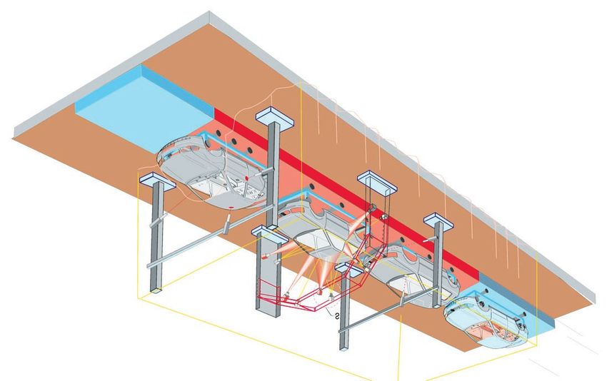
ABIS (Automatical Body Inspection System) image is evaluated by spatial phase shift [7]
is a system to automatically check car-bodies from a single sinusoidal fringe pattern that
on the production line for dents and ripples. is projected by a flash light.
It is designed in collaboration of the AUDI • Defect Detection: The huge amount of data
AG Ingolstadt, Steinbichler Optical Technolo- has to be reduced. Each sensor has its own
gies Neubeuern, TECMATH/TECINNO GmbH processing unit which detects candidates for
Kaiserslautern, the Institute for Techno- and potential defects. Only range images which
Business Mathematics (ITWM) Kaiserslautern possibly contain relevant defects are trans-
and the Chair for Optics of the University of mitted to the analysis and classification unit.
Erlangen-Nuremberg. Two components are in- • Defect analysis and classification: The
tegrated into the production line (Fig. 1): a sen- analysis unit extracts certain features from
sor portal with range sensors that scan the whole the candidate data. These features are eval-
surface of the body and a portal with robots that uated by a self-teaching case-based reason-
mark regions with detected defects. The process- ing (CBR) algorithm [1]. The CBR system
ing chain covers the following tasks: decides whether the candidate really is a de-
• Identification of the car type: The camera fect and if so, whether it is relevant (class A
and robot positions are individually adapted or B defect).1
to the type of car-body that enters the sensor
portal. Only those car-bodies are checked, 1 Class A defects are visible before varnishing, class B
the type of which is known to the system. defects only afterwards. Class C defects are never visible.Figure 1: Integration of ABIS into the production line.
This paper describes the defect detection unit.
The most challenging aspect is the fact that up
to the present no definition for relevant defects is
known. Thus, our first goal was to find out what
the system should search for. Figure 2 points
out the difficulty of this task. It shows profile
data of a scanned metal sheet with a tiny out-
dent (“blain”) that is only a few pixels wide and
10 µm high. Because of a 15 µm mean noise
amplitude the “blain” is nearly invisible in the
raw data. After smoothing with a 5 × 5 Gaus-
sian filter kernel a slight distortion of the sheet
curvature in the range of pixels 28–52 appears.
Figure 2: Extract of scanned sheet profile with However, is this really the “blain” (compare with
a 10 µm “blain” (upper: raw data; lower: Fig. 4)? We solved the problem in two steps:
smoothed with a 5 × 5 Gaussian filter kernel). 1. A method to visualize the defects was de-
Figure 4 shows the visualization results for that veloped.
data. 2. The visualization method was used to de-
sign a fast detection algorithm.
• Marking system: If class A or B defects Because of the speed of the production line
are detected, the corresponding regions on and the large number of images to be analyzed,
the body are painted with chalk by robots. each image has to be processed in less than 2.4
These regions are then polished manually. sec in the final system.
The results of the classification unit are sup- Most of the following figures originally are in
posed to help objectifying the whole process of color. Since some of the gray scale prints are
defect detection by revealing the relations be- difficult to interpret, we recommend to visit our
tween the geometrical dimensions of a defect and web sites.2
its visibility. Until now human inspectors esti- 2 http://www.physik.uni-erlangen.de/optik/haeusler/
mate the relevance of a defect. This approach is people/sbk/visualize_e.html and http://www.physik.uni-
rather subjective, of course. erlangen.de/optik/haeusler/people/sbk/detection_e.htmlFigure 3: Visualization of two 300 µm in-dents on a sheet metal (field of view 30 × 15 cm2 ), a) color
coded range image, b) geometrically smoothed and rendered with simulation of grazing incidence
of light, c) 2nd derivative of smoothed data rendered with grazing incidence, d) previous image after
threshold operation: the detected dents are marked (originally in blue and red).
2 Related Work ometry. The Diffracto system is commercialized
with the trademark D Sight.3 Since the previous
methods do not acquire any geometrical data,
The “dents and ripples” problem was first solved they are suitable for qualitative measurements
by 2-d imaging for shiny surfaces like painted or only. Thus, they are mainly used to visualize
anointed sheet metals. Such methods detect cur- defects. Beyond this, they require reflective sur-
vature variations by observing the reflected light. faces. Unpainted car-bodies must be coated with
The spatial orientation of the reflected beam de- a fluid film of water or oil in advance. In order
pends on the local orientation of the observed to overcome these limitations, Daimler Benz AG
surface, so that special efforts are required to Germany in cooperation with Carl Zeiss GmbH
keep the sensor within the beam. Nissan Motor developed a car-body inspection system that uses
Corp. introduced a system that uses a manipu- 3-d sensors for data acquisition [3]. However,
lation stage for that purpose [4]. The surface is this system only is used internally and has never
illuminated by a laser line and a linear CCD ar- been commercialized. ABIS likewise uses range
ray detects distortions of the reflected line which sensors to examine diffusely reflective surfaces
are caused by local curvature. Sira Ltd. U.K. and to quantify the detected defects.
[8], Siemens AG Germany [9] and Diffracto Ltd.
Canada [10] use a retroreflective screen to reflect
the light back towards its source. The sensor is 3 Defect Visualization
placed near to the light source and observes the
retroreflected light. Intensity variations due to Figure 3 a) shows a color coded range image
local slope variations are amplified by the im- taken from a sheet metal with two in-dents on
perfection of the retroreflector. The Sira system it (dark colors indicate low z-values). Although
scans the surface pointwise. One photo multi- the dents are rather deep (approx. 300 µm), they
plier is placed in the direction of the beam re- are nearly invisible. In order to solve the visual-
flected by an undisturbed surface, another one in ization problem we considered how a human ob-
its dark field. Siemens and Diffracto use CCD server would check a sheet metal for defects. He
cameras to directly acquire 2-d images, which
are special kinds of derivatives of the surface ge- 3 http://www.diffracto.com/products/dsight/dsight.htmprobably would orient the sheet in such a way
that the light would tangentially graze the in-
spected part of the surface. Obviously, small dis-
turbances of the surface curvature become bet-
ter and better visible with increasing angle be-
tween the direction of illumination and observa-
tion. Thus, we simulate observation of the virtual
surface by grazing incidence of light (see Sec. 5).
Applying this technique to the original range im-
age mainly enhances distortions with high spa-
tial frequency, like noise and Moiré structures
caused by aliasing. To make the defects visible,
we smooth the image in advance with a special Figure 4: Visualization of 10 µm “blains” on
filter for geometric data [5, 6] that generates al- a wheel arch (left: smoothed range image ren-
most no artifacts dered with grazing incidence of light, middle: 2nd
Figure 3 b) shows the smoothed data of Fig. derivative rendered with grazing light, right: re-
3 a) with blue light virtually coming from the left sult of threshold operation).
side and red light coming from the right. In the
original color image those parts of the surface
ized by simulating grazing incidence of light. In
which are slightly slanted to the left are rendered
Fig. 3 c) the differentiation was carried out twice.
in blue, those which are slanted to the right are
Now the defects are detected by a simple thresh-
red and only those regions which are strictly or-
old operation (see Fig. 3 d).
thogonal to the observation direction are black.
The dents are clearly visible now. However, the In practice, this method displays good results,
curvature of the sheet itself disturbs automatic even if the depth of the defects is smaller than
detection of such defects, in particular if they the sensor noise. Figure 4 demonstrates this for
are small. Fortunately, the sheets usually have at a range image with 10 µm “blains” and 15µm
least one direction with low curvature. If the sig- noise. Figure 2 shows a horizontal cross sec-
nal is processed only in that direction,4 the intrin- tion through the raw and the smoothed data of
sic curvature can be eliminated by a high pass fil- one of the “blains”. Because of costly geometric
ter. We investigated several types of filters. Best smoothing the visualization takes a few minutes
results were achieved with a special kind of dif- on an Intel Pentiumr II 300 CPU.
ferentiation. The image is shifted in processing
direction (16 pixels horizontally in Fig. 3 c) and
then subtracted from the unshifted one. The re- 4 Fast Defect Detection
sult is a very fast and effective band pass filter
that produces almost no artifacts. If the image The algorithm is based on the described visual-
is shifted d pixels, the filter shows maximum re- ization method. The method is simplified in or-
sponse for structures with wavelength d2 . This fil- der to speed up processing time. Since the sim-
ter is applied several times to the smoothed range ulation of grazing incidence of light only pro-
image. cesses surface normals, it is sufficient to compute
the normals from the unfiltered range image and
If the sheet surface can be approximated by a
smooth the normals instead of smoothing the ge-
polynomial of order n, the differentiation has to
ometry itself. This is easier, faster and produces
be applied n − 1 times. Because of the grazing
fewer artifacts. A hierarchy of three different
incidence simulation the total order of differen-
resolutions for covering defects of different lat-
tiation is n. The resulting image is again visual-
eral size (small “blains”, as well as large sized
4 This means that the illumination direction coincides undulations) is realized by averaging blocks of
with the direction of minimum curvature. 2 × 2, 4 × 4, or 8 × 8 pixels (see Fig. 6 a, d, g,5 Simulation of Grazing Inci-
dence of Light
Grazing incidence simulation is done by sim-
ply computing the inner products of the inci-
dent light vector (processing direction) and the
surface normals. Negative values are indicated
by blue, positive values by red light. Theoret-
ically, it would be possible to apply an addi-
tional differentiation instead of this procedure.
But if we do so, we have to smooth the geom-
etry directly, with all the mentioned disadvan-
tages. Furthermore, the virtual light may come
Figure 5: Range image of a sheet metal with a in from arbitrary directions, whereas the direc-
laterally large sized dent, a) simulation of graz- tion of differentiation is limited by the sampling
ing incidence of light, b) 2nd derivative rendered grid. Another advantage of the grazing incidence
with grazing incidence, c) result of visualization approach is its normalized range of output val-
method, d) result of lowest resolution of the fast ues, which stabilizes the threshold operation.
detection algorithm.
resp. b, e, h, resp. c, f, i). The final algorithm
runs the following steps for each resolution: 6 Automatic Threshold
1. Compute surface normals.
2. Compute mean direction of minimum cur-
The threshold for step 6 of the detection algo-
vature (processing direction, see Sect. 8).
rithm determines the sensitivity of the system.
3. Smooth normals by weighted averaging of
The maximum sensitivity is limited by the sen-
adjacent normals (4–6 iterations).
sor noise and by remainders of an incomplete
4. Simulate grazing incidence of light (see
compensation of the intrinsic surface curvature.
Sec. 5).
This limit increases with the mean variation of
5. Differentiate result (2–4 times with 4–6 pix-
the signal of the last derivative (step 5). Thus,
els shift).
the threshold is automatically adjusted propor-
6. Subtract mean intensity from the last deriva-
tionally to this mean variation. The proportion-
tive and apply threshold operation (Sec. 6).
ality factor is determined heuristically. The user
7. Analyze shape of marked regions (Sec. 7).
solely specifies a minimum threshold that deter-
The last step is necessary to remove noise and mines the maximum sensitivity for nearly flat
other artifacts from the threshold images. A de- surfaces and low noise.
fect is detected if any marked (red or blue) pixel
Figure 6 shows the results of a single range
remains. Since it is more efficient to differenti-
image with constant (a–c) and automatic (g–i)
ate single valued arrays than vectors, steps 4 and
threshold. The intrinsic surface curvature is not
5 are interchanged with respect to the visualiza-
perfectly compensated for, so that a constant
tion algorithm.
threshold detects this effect in the lowest reso-
Figure 5 compares the results of the visualiza- lution (c). This problem does not occur if the
tion method (Sec. 3) with the fast detection algo- threshold is automatically adjusted (i). Although
rithm. Although the latter is at least 100 times the sensitivity is impaired in this case, detection
faster, it shows less noise. of real defects is still possible (compare b and h).Figure 6: Results of all resolutions on a rear mudguard (the black rectangle in upper left of each image
masks the fuel cap, a part of the wheel arch is visible in each lower right corner), (a–c) with constant
threshold, (d–i) with automatic threshold, (d–f) before shape analysis, (g–i) after shape analysis.
7 Shape Analysis 8 Computation of Principal
Directions
Shape analysis is used to eliminate artifacts
The described visualization and detection meth-
caused by noise, Moiré, boundary distortions
ods achieve best results if the direction of vir-
and sharp edges of the surface. It is inspired by
tual illumination touches the surface in parallel
the observation that humans, after some practice,
to the direction of minimum curvature. For this
are usually able to distinguish defects from arti-
purpose the principal directions have to be com-
facts by the shape of the marked regions. Real
puted. Usually this is done by approximating
defects are usually compact, not elongated like
Chebychev polynomials and analyzing them by
Moiré structures or artifacts from boundary ef-
means of differential geometry [2]. However,
fects and sharp edges. They always consist of
this approach is very expensive and sensitive to
two complementary components (red and blue),
noise. We use a new method which is very sim-
if they are sufficiently far away from the bound-
ple, robust and flexible, since it can be applied
ary. Thus, the shape analysis algorithm removes
both to grid data like range images and unstruc-
marked regions that exceed a certain aspect ratio
tured data like triangle meshes.
or are isolated with a distance to the boundary
larger than a certain limit. We assume that the sampled data approximate
a smooth surface. If triangle meshes are con-
Figure 6 displays the results of a single range sidered, the vertices are sampled surface points.
image before (d–f) and after (g–i) shape analy- Grid data sets are treated like triangle meshes
sis. The outputs of step 6 show artifacts caused as well. The sampling density shall be high
by Moiré distortions, boundary effects and the enough to neglect the variations of surface cur-
sharp edge at the wheel arch (d–f). After shape vature between adjacent data points. If this
analysis only defects in the vicinity of the wheel is true, the underlying surface can be approx-
arch (h) and of the masked fuel cap (i) remain. imated more accurately by a mesh of circularFigure 7: Cross section S through a constantly Figure 8: A vertex V on a curved surface with
curved surface. neighbors Vi placed in principal directions~ξ1 and
~ξ2 (idealization).
arcs. First, we show how easily curvature can
be estimated when using this simplified model.
of a vertex V with four neighbors Vi , 1 ≤ i ≤ 4,
Figure 7 shows a cross section S through a con- and the associated vertex normals ~n and ~n j that
stantly curved object surface between two adja-
perfectly fit a mesh of arcs. The neighbors Vi
cent vertices (data points) Vi and Vj . The curva-
are placed on arcs that touch V tangentially to
ture ci j of the curve S is (ci j > 0 for concave and
the principal directions ~ξ1 and ~ξ2 of the assumed
ci j < 0 for convex surfaces)
surface. Obviously, ~ξ1 and ~ξ2 are coaxial to the
1 αi j cross product of~n1 and ~n2 or~n3 and ~n4 , resp.:
ci j = ± ≈ ± ≈ ± arccos(~ni ·~n j ), (1)
r di j
~ξ1 = ~n1 ×~n2 , ~ξ2 = ~n3 ×~n4 . (3)
which can easily be computed if the surface nor- k~n1 ×~n2 k k~n3 ×~n4 k
mals~ni and~n j are known (they can be computed
from the normals of the triangles meeting at Vi ). In a general mesh (not a range image), a vertex
The principal curvatures κ1 (i) and κ2 (i) of Vi are has an arbitrary number of neighbors. Since the
the extreme values of ci j with regard to all its length of the product vectors ~ni ×~n j increases
neighbors Vj : with curvature, the principal directions can be es-
timated by taking the longest (maximum curva-
κ1 (i) ≈ min(ci j ) and κ2 (i) ≈ max(ci j ). (2)
j j ture) and the shortest (minimum curvature) vec-
tor. Notice that the maximum vector points in
The surface normals are computed in advance direction of minimum curvature and vice versa.
(see Sec. 4), hence it is possible to eliminate Because of noise, the computation of the min-
noise by smoothing the normals without any in- imum vector (direction of maximum curvature)
terference of the data points. is usually very unstable. If ~ξ2 is the direction of
It can be shown that approximation of a minimum curvature, then it is better to calculate
mesh of circular arcs requires a sampling den- the maximum direction by
sity which is at least four times higher than the
smallest object detail to be modeled. This means ~ξ1 = ~ξ2 ×~n.
that the minimum sampling rate must be twice (4)
the theoretical minimum given by the Nyquist
frequency. Since the lateral size of the defects Figure 9 shows the directions of minimum cur-
is much larger than the sampling distance, this vature of a triangular surface that was recon-
condition is always fulfilled. structed from multiple range images. Although
While the principal curvatures are simply the mesh is thinned, the computation shows good
computed by inner products of the normals, the results with low noise. The computation of prin-
corresponding cross products define the princi- cipal directions for all data points of a range im-
pal directions. Figure 8 shows the special case age of size 700 × 500 only takes approx. 100 ms.References
[1] A. Aamodt and E. Plaza. Case-
based reasoning: Foundational issues,
methodological variations, and system ap-
proaches. Artificial Intelligence Communi-
cations, 7(1):21–40, 1994.
[2] P. J. Besl and R. C. Jain. Invariant surface
characteristics for 3d object recognition in
range images. Computer Vision, Graphics,
and Image Processing, 33:33–80, 1986.
[3] B. Dörband, R. Köthe, and A. Zilker.
Streifenprojektion prüft in Echtzeit mit 5
µm Auflösung. Werkstatt und Betrieb,
128(3), 1995.
[4] G. Häusler and K. Engelhardt. Verglei-
chende Studie zur automatisierten Lack-
fehlerbestimmung. Expertise, University of
Erlangen-Nürnberg, August 1987.
[5] G. Häusler and S. Karbacher. Reconstruc-
tion of smoothed polyhedral surfaces from
multiple range images. In B. Girod, H. Nie-
mann, and H.-P. Seidel, editors, 3D Image
Analysis and Synthesis ’97, pages 191–198,
Figure 9: A surface that was reconstructed from Sankt Augustin, Germany, 1997. Infix Ver-
multiple range images (upper) and detail of the lag.
triangle mesh with vectors that define directions [6] S. Karbacher. Rekonstruktion und Mod-
of minimum curvature assigned to each vertex ellierung von Flächen aus Tiefenbildern.
(lower). PhD thesis, University of Erlangen-
Nürnberg, Shaker Verlag, Aachen, 1997.
9 Conclusions [7] M. Kujawinska. Spatial phase measure-
ment methods. In David W. Robinson
and Graeme T. Reid, editors, Interferogram
We introduced a new method to visualize small Analysis: Digital Fringe Pattern Measur-
defects on unreflective surfaces like unpainted ment Techniques, pages 141–193. Institute
sheet metals or plastic panels. Satisfying re- of Physics Publishing, Bristol, 1993.
sults are achieved, even if the depth of a defect [8] Sira Ltd. Car paint inspection system. Out-
is smaller than the sensor noise. A fast multi- line description, Chislehurst, U.K., April
resolution detection algorithm is based on that 1987.
method. Processing a 700 × 500 range image [9] H. Marguerre. Ein neues inkohärentes
with three resolutions takes less than 1.5 sec on Schlierenverfahren mit Retroreflektor. Op-
an Intel Pentiumr II 450 CPU. tik, 71(3):105–112, 1985.
[10] R. L. Reynolds, F. Karpala, D. A. Clarke,
and O. L. Hageniers. Theory and applica-
tions of a surface inspection technique us-
10 Acknowledgement ing double-pass retroreflection. Optical En-
gineering, 32(9):2122–2129, 1993.
This work was sponsored by “Bayrische
Forschungsstiftung”.You can also read