VMD Images and Movies Tutorial
←
→
Page content transcription
If your browser does not render page correctly, please read the page content below
University of Illinois at Urbana-Champaign
Beckman Institute for Advanced Science and Technology
Theoretical and Computational Biophysics Group
Computational Biophysics Workshop

  VMD Images and Movies
        Tutorial

                                                           Alek Aksimentiev
                                                                   John Stone
                                                                  David Wells
                                                          Marcos Sotomayor
                                                                      FEB 2012

                  A current version of this tutorial is available at
                   http://www.ks.uiuc.edu/Training/Tutorials/
        Join the tutorial-l@ks.uiuc.edu mailing list for additional help.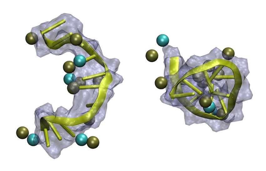
CONTENTS                                                                                                        2

Contents
1 Working with Still Frames                                                                                      5
  1.1 Graphical Representation Resolution       .   .   .   .   .   .   .   .   .   .   .   .   .   .   .   .    5
  1.2 Colors and Materials . . . . . . . . .    .   .   .   .   .   .   .   .   .   .   .   .   .   .   .   .    5
  1.3 Depth Perception . . . . . . . . . . .    .   .   .   .   .   .   .   .   .   .   .   .   .   .   .   .    7
  1.4 Rendering . . . . . . . . . . . . . . .   .   .   .   .   .   .   .   .   .   .   .   .   .   .   .   .    9
  1.5 Volumetric Data . . . . . . . . . . .     .   .   .   .   .   .   .   .   .   .   .   .   .   .   .   .   10
  1.6 Clipping Planes . . . . . . . . . . . .   .   .   .   .   .   .   .   .   .   .   .   .   .   .   .   .   13
  1.7 Visualizing Large Systems . . . . . .     .   .   .   .   .   .   .   .   .   .   .   .   .   .   .   .   17

2 Working With Trajectories                                                    18
  2.1 Basics . . . . . . . . . . . . . . . . . . . . . . . . . . . . . . . . . 18
  2.2 Advanced Trajectory Topic . . . . . . . . . . . . . . . . . . . . . 20
  2.3 Making Movies . . . . . . . . . . . . . . . . . . . . . . . . . . . . 25
CONTENTS                                                                       3

Introduction
 This tutorial is designed to give users of VMD an introduction to advanced
techniques for making custom images and movies. The tutorial assumes that
you already have a working knowledge of VMD. For the accompanying VMD
tutorials go to:
http://www.ks.uiuc.edu/Training/Tutorials/
This tutorial has been designed specifically for VMD 1.8.5, and should take about
3 hours to complete in its entirety.

 The tutorial is subdivided into two separate units. In the first unit, we will
look at the many options in VMD for the setup and production of images. The
second unit is dedicated to trajectory use and the production of movies.

 The Visualizing Molecules with VMD tutorial, available at http://www.scripps.edu
/rc/training/unixslides/vmd.pdf, covers graphical representations in more de-
tail.

 If you have any questions or comments on this tutorial, please email the TCB
Tutorial mailing list at tutorial-l@ks.uiuc.edu. The mailing list is archived at
http://www.ks.uiuc.edu/Training/Tutorials/mailing list/tutorial-l/.
CONTENTS                                                                      4

Required programs
The following programs are required for this tutorial:

   • VMD: Available at http://www.ks.uiuc.edu/Research/vmd/ (for all plat-
     forms)
   • POV-Ray: Available at http://www.povray.org/download/ (for all plat-
     forms)
   • MSMS: Available at http://www.scripps.edu/pub/olson-web/people/
     sanner/html/msms home.html
   • VMDMovie: This plugin ships with VMD. However, please see
     http://www.ks.uiuc.edu/Research/vmd/plugins/vmdmovie/ for platform-
     specific information regarding MPEG generation.

Getting Started
 You can find the files for this tutorial in the imgmvtut-files directory. Below
you can see in Fig. 1 the files and directories of imgmvtut-files.

                                            dna.pdb
                                            1VS6.pdb
                                            dna.psf
                                            pore.psf
                                            trajectory.dcd
                                            pore.dcd
                                            pore.mpg
                                            arrows.mpg
                                            2views.mpg
               imgmv-tutorial-files
                                            noupdate.mpg
                                            update.mpg
                                            usermovie.mpg
                                            volmap-density.dx
                                            pmepot.dx
                                            pore.tcl
                                            marshmallow.tcl
                                            makingmovies-restart.tcl
                                            usermovie.tcl

                Figure 1: Directory structure of imgmvtut-files

 To start VMD type vmd in a Unix terminal window, double-click on the VMD
application icon in the Applications folder in Mac OS X, or click on the Start
→ Programs → VMD menu item in Windows.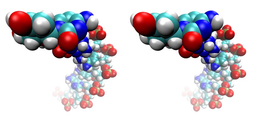
1   WORKING WITH STILL FRAMES                                                    5

1     Working with Still Frames
In this section, we will look at some of the variety of ways VMD can work with
still frames.

1.1    Graphical Representation Resolution
 Objects are drawn with an adjustable resolution, allowing users to balance fine-
ness of detail with drawing speed. The resolution setting directly controls the
smoothness of the surface molecular representation, and the quality of lighting,
texturing, and surface shading for interactive display. The resolution setting
also affects the quality of external renderers, but with important differences
which will be discussed later.

    1 Load the files dna.pdb and dna.psf.

    2 Show just the DNA, and use the VDW drawing method.

    3 Zoom in on one or two of the atoms, either by using the scroll wheel on
      your mouse, or by using Mouse → Scale Mode (shortcut s) and clicking
      and dragging.

    4 Notice that with the default resolution setting, the “spherical” atoms
      aren’t looking very spherical. In the Graphical Representations window,
      click on the representation you set up before for the DNA, and click on the
      Draw Style tab. Try adjusting the Sphere Resolution setting to something
      higher, and see what a difference it can make. (See Fig. 2.)

 Many of the drawing methods have a resolution setting. Try a few different
ones. When producing images, you can usually raise the resolution until it stops
making a visible difference.

1.2    Colors and Materials
 Nearly all aspects of the display are user-adjustable, including background and
display mode colors, and material properties of the objects drawn. Material
properties control the way that VMD calculates surface lighting and opacity of
displayed objects. Material properties can be used to create dull matte surfaces,
eye catching shiny or glass-like surfaces, and transparent ghost-like objects, each
suiting different needs. Dull, matte, or diffuse materials are frequently used for
background objects or low importance areas of structure, when one wishes to
provide context but not draw too much attention, and are also well suited to
production of high quality grayscale images. Shiny or glassy materials are useful
to attract attention, and emphasize surface curvature with specular highlights.
Shiny materials may be too “busy” for grayscale images, and tend to be best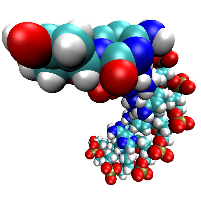
1   WORKING WITH STILL FRAMES                                                          6

    (a) Low resolution: Sphere Resolution    (b) High resolution: Sphere Resolution
    set to 8                                 set to 28

                  Figure 2: The effect of the resolution setting.

suited to use in color images. Opacity can be used to deemphasize areas of
structure or to provide context, and can be particularly useful when superim-
posing several objects.

    1 In the VMD Main window, choose Graphics → Colors. . . . Look through
      the Categories list. All display colors, e.g. the color of phosphorus atoms
      when coloring by name, are set here.

    2 Now we will change the background color. In Catagories, select Display.
      In Names, now click Background. Finally, choose white in Colors.

    3 When making a figure for a publication, we often don’t want the axes
      showing. Select Display → Axes → Off to disable them.

    4 You may have noticed the Material menu in the Graphical Representations
      window. Choose the DNA representation you made above, and experiment
      with the Material menu.

                   GLSL. Now is a good time to try out the GLSL Render Mode,
                   if your computer supports it. In the VMD Main window, choose
                   Display → Rendermode → GLSL. This mode uses your 3D graphics
                   card to render the scene with real-time raytracing of spheres and
                   alpha-blended transparency; see Fig. 3 for an example.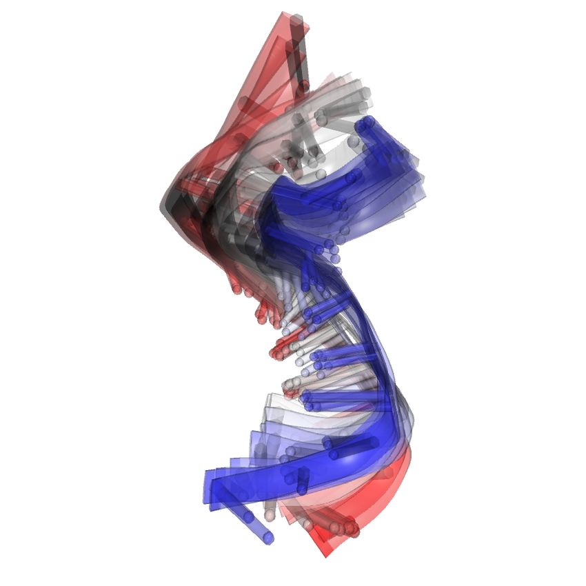
1   WORKING WITH STILL FRAMES                                                     7

      (a) The default transparent material.        (b) A user-defined material.

                 Figure 3: Examples of different material settings.

    5 Now we’ll make a new material. In the VMD Main window, choose Graph-
      ics → Materials. . . . In the window that appears, you’ll see a list of the
      materials you just tried out, and their adjustable settings. Click the Create
      New button, and give it the following settings:

                                    Setting     Value
                                    Ambient     0.62
                                    Diffuse     1.00
                                    Specular    0.87
                                    Shininess   0.85
                                    Opacity     0.11

       See if you can reproduce Fig. 3(b) (Hint: use two representations of DNA.)

1.3     Depth Perception
 Since the systems we are dealing with are three dimensional, VMD has multiple
ways of representing the third dimension. In this section we will explore the use
of VMD features which enhance or diminish depth perception.

    1 The first thing to consider is the projection mode. In the VMD Main
      window, click the Display menu. Here we can choose either Perspective
      or Orthographic. In perspective mode, things nearer the camera appear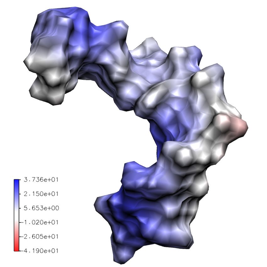
1   WORKING WITH STILL FRAMES                                                           8

      larger. Although perspective projection provides strong size-based visual
      depth cues, the displayed image will not preserve scale relationships or
      parallelism of lines, and objects very close to the camera may appear dis-
      torted. Orthographic projection preserves scale and parallelism relation-
      ships between objects in the displayed image, but greatly reduces depth
      perception. See Fig. 4 to see the difference this can make.

              (a) Perspective                          (b) Orthographic

Figure 4: Comparison of perspective and orthographic projection modes. These
were taken from above and to the side of the DNA.

                  Orthographic versus Perspective Mode. Orthographic mode
                  tends to be more useful for analysis, because alignment is easy to
                  see, while perspective mode is often used for producing figures and
                  stereo images.

    2 Another way VMD can represent depth is through so-called “depth cue-
      ing”. Depth cueing is used to enhance three-dimensional perception of
      molecular structures, particularly with orthographic projections. Choose
      Display → Depth Cueing in the VMD Main window. With depth cueing
      enabled, objects further from the camera are blended into the background.
      Depth cue settings are found in Display → Display Settings. . . . Here you
      can choose the functional dependence of the shading on distance, as well
      as some parameters for this function.

                  Linear Depth Cueing. If you choose Cue Mode → Linear in the
                  Display Settings window, you can achieve dramatic shading across
                  the subject of your figure by choosing the Cue Start and Cue End
                  parameters. See Fig. 5 for an example of this.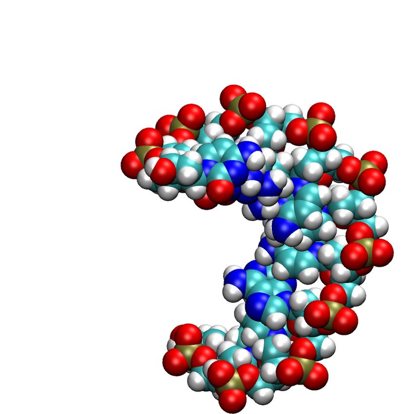
1   WORKING WITH STILL FRAMES                                                  9

Figure 5: Stereo image of DNA, also showing linear depth cueing, with Cue
Start = 1.5, Cue End = 2.75.

    3 Finally, VMD can also produce stereo images. In the VMD Main win-
      dow, look at the Display → Stereo menu, showing many different choices.
      Choose SideBySide, and return to Perspective mode as well. You should
      get something like that shown in Fig. 5

1.4    Rendering
 By now we’ve seen some techniques for producing attractive figures in VMD
interactively. In this section, we’ll explore the use of the snapshot feature and
external rendering programs to produce high quality image files. The interactive
graphics display in VMD is performed by OpenGL and uses fast-but-elementary
geometry, lighting, and transparency algorithms. In many cases, the interactive
renderings created by VMD are adequate for use in presentations, movies, and
small figures. The “snapshot” renderer saves the on-screen image and is handy
for these cases. When one desires higher quality antialiasing, transparency,
lighting, perfectly curved spheres, solid clipped volumes, or extremely high res-
olution images, renderers such as Tachyon and POV-Ray are better choices.
Several of the supported renderers use ray tracing for high quality rendering of
curved surfaces. Most of the supported renderers perform lighting calculations
at every pixel, and so there’s less need to set the graphical representation res-
olution parameters to high values. Renderers such as Tachyon and POV-Ray
actually perform better and create nice images with very conservative repre-
sentation resolution settings. Other rendering modes such as STL and VRML
can be used to export the VMD molecular scene to a variety of rendering and
animation tools, or for printing of 3-D solid models.

    1 Rendering is a simple matter. Once you have the scene set the way you
      like it, simply choose File → Render. . . in the VMD Main window. In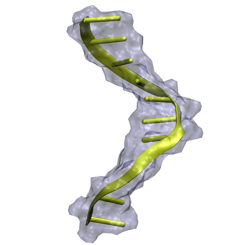
1   WORKING WITH STILL FRAMES                                                          10

      the File Render Controls window that appears, you choose the renderer
      to use, choose the file name, and click Start Rendering.

                   Command Line. The Tk Console can be useful for setting up your
                   scene in a precise way. Using display resize  , you can
                   set the size of the display window, and therefore also the size of
                   the rendered image. Using the rotate and scale commands, you
                   can change the camera angle and zoom. There is also a render
                   command — the menu command above is simply a GUI front end.

    2 Now let’s actually render something. Try rendering the scene you have set
      up currently, using the renderers snapshot, TachyonInternal, and POV3.

                   Renderers. The snapshot renderer saves exactly what is already
                   showing in your display window — in fact, if another window over-
                   laps the display window, it will show up in the rendering as well!
                   The other renderers reprocess everything, so it may not look exactly
                   as it does in VMD. In particular, they don’t “clip”, or hide, objects
                   very near the camera. If you select Display → Display Settings. . .
                   in the VMD Main window, you can set Near Clip to 0.01 to get a
                   better idea of what will appear in your rendering.

    3 OK, now for something more challenging. Try to reproduce Fig. 6 as best
      you can. Think about which parts of the system to show, the drawing and
      coloring method, the projection mode, and the materials.

1.5    Volumetric Data
 VMD has the ability to compute and display volumetric data. Volumetric data
is data that is a function of position, e.g. density, potential, solvent accessibil-
ity, stored as a 3-D grid of values. VMD can display volumetric data in a few
different ways. For this section, please turn GLSL rendering off, if it is on.

                   Creating Volumetric Data. VMD has a number of analysis plug-
                   ins that compute volumetric data, notably the VolMap and PMEpot
                   plugins.

    1 Load the file volmap-density.dx by selecting our molecule in the VMD
      Main window, clicking File → Load Data Into Molecule. . . , then browsing
      to the file.

                   volmap-density.dx. This volmetric data set was generated by the
                   VolMap plugin from a 1 ns simulation of the system we’ve been
                   looking at, and shows the mass density of DNA averaged over the
                   trajectory.
1 WORKING WITH STILL FRAMES 11
Figure 6: Example of POV3 rendering.
2 Our molecule now has one volumetric data set associated with it, as in-
dicated by the “1” in the Vol column of the VMD Main window. Now
we need a representation to display it. Create a new representation, and
select VolumeSlice as the Drawing Method.
3 With the new representation still selected, set Slice Axis to Y, Render
Quality to Medium, and Coloring Method to Volume.
4 Turn off all other representations, then type the following into the Tk
Console window:
display resetview
rotate x by -90
Play with the Slice Offset slider, which adjusts the y-coordinate of the slice.
Different colors represent different numerical values of the volumetric data,1 WORKING WITH STILL FRAMES 12
in this case mass density. When coloring by Volume, the color scale can
be set in the Trajectory tab of the Graphical Representations window.
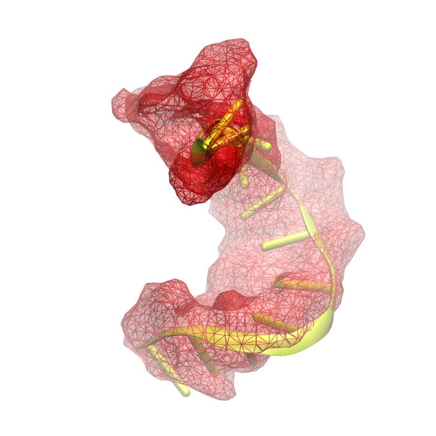
(a) Volume slices. (b) Mesh and transparent solid sur-
faces at isovalue 0.33.
Figure 7: Different ways of showing volumetric data of DNA mass density.
5 Now make a similar slice representation for the x- and z-directions as well,
and rotate you view with the mouse so that all three planes are visible.
Fig. 7(a) shows an example with slice planes normal to the x- and y-axes.
6 Now for a more three-dimensional way of representing the data. Hide
the current representations, then create a new one using the Isosurface
drawing method. In the Draw menu, select Solid Surface. Now, you can
see a surface of constant volumetric value, chosen using the Isovalue slider.
As you choose higher values, you see the surface shrinks down around a
core where the most average mass was located. Fig. 7(b) shows such an
isosurface, represented by both a wire mesh and a transparent surface.
7 Another common way to represent volumetric data is by coloring other
representations based on it. Load the file pmepot.dx by selecting your
current molecule, and choosing File → Load Data Into Molecule. . . in the
VMD Main window.
pmepot.dx. This file was generated from the same trajectory as the
other volumetric dataset you’ve been using, this time from the last
frame alone. As its name implies, it was made using the PMEpot
plugin, which calculates electrostatic potential.1 WORKING WITH STILL FRAMES 13
8 Now hide your current representations, and create a new one showing only
DNA, with MSMS drawing style and Volume coloring style. The DNA
surface is now colored based on the volumetric data value at each surface
point. The color scale range is automatically set, but can be changed in
the Trajectory tab of the Graphical Representations window.
9 We’ll use the Color Scale Bar VMD plugin to show the color scale of the
volumetric data. Choose Extensions → Visualization → Color Scale Bar in
the VMD Main window.
10 Enable the Autoscale option, set the label color to black, and click Draw
Color Scale Bar. This plugin will create a new molecule named Color Scale
Bar that is “fixed”, meaning when you rotate or scale the scene, the color
bar doesn’t change.
11 You can move the color bar by unfixing its molecule and fixing the DNA
molecule, then using the Translate mouse mode (shortcut T). Recall that
a molecule is fixed or unfixed by double-clicking the “F” directly to the
left of its name in the VMD Main window. An example is shown in Fig. 8.
Figure 8: Example of coloring by volumetric data and use of the Color Scale
Bar plugin.
1.6 Clipping Planes
In this section, we will learn one of the most useful techniques for producing
clear figures: the clipping plane. Clipping planes allow us to look at cross-
sections of the objects displayed, and can be applied very flexibly. We will learn
how to use them by going through the steps of making Fig. 9.1 WORKING WITH STILL FRAMES 14
Figure 9: A three-dimensional contour plot, made through the use of clipping
planes.
1 Start a fresh VMD session, and reload the files dna.psf, dna.pdb, and
volmap-density.dx.
2 Create the representations in the following table. For each, select Draw →
Solid Surface and Show → Isosurface in the Draw style tab. Once they’re
set up, you should see only a blue shell.
Drawing Method Isovalue Coloring Method
Isosurface 1.0 ColorID 1 (red)
Isosurface 0.6 ColorID 7 (green)
Isosurface 0.2 ColorID 0 (blue)
3 Now enter the following commands in the Tk Console:1 WORKING WITH STILL FRAMES 15
mol clipplane status 0 0 0 2
mol clipplane status 0 1 0 2
mol clipplane status 0 2 0 2
Let’s decipher this a bit. Every mol clipplane command is of the form
mol clipplane .
Here, we have used the status command, which we use to enable the
clipping planes. Thus, the first line refers to the first clipping plane of the
first representation of the first molecule. The final 2 is the new status of
each clip plane. Table 1 summarizes this command’s usage.
Possible s
status 0 (off), 1 (on), 2 (on, solid surface; material inherited from representation)
normal " ", a vector pointing normal to the surface
center " ", a vector pointing to the center of the surface
color " ", an RGB triple specifying the color of the surface, if it is solid
Table 1: Summary of mol clipplane usage.
Multiple Clipping Planes. All of these numbers you give the mol
clipplane commands show how flexible the command is — one
may define up to six different clipping planes per representation!
4 Let’s check the current settings of the clipping planes. Type the com-
mands:
mol clipplane center 0 0 0
mol clipplane normal 0 0 0
and likewise for the other two clipplanes. By providing no new value, the
command now print the current value instead of setting a new one. You
should find that all clipplanes are centered at the origin, and with normal
vector in the z-direction.
5 Now we’ll use a trick to set the center and normal vectors interactively,
using the Clipping Plane Tool VMD Plugin. Select Extensions → Visual-
ization → Clipping Plane Tool in the VMD Main window. This tool will
modify clipping planes of the molecules selected in the Apply To menu.
The Edit Clip Plane buttons select which clipid will be edited. However,
all representation clipping planes will be edited together, i.e. all the clip-
ping planes we’ve created will get the same normal and center — exactly
what we want.1 WORKING WITH STILL FRAMES 16
6 You should now see cross-sections of the isosurfaces you created. Rotate
down with the mouse. The clipping plane stays parallel to the screen,
letting us choose the normal vector (the flip button inverts this vector).
Try to set the normal vector so that we get a nice cross-section of the
isosurfaces.
7 Now, adjust the position of the plane in the normal direction by using the
Distance slider. Try to cut right through the center of the isosurfaces.
8 When you think you have a nice cross-section, click the Keep Aligned with
Screen button to turn this feature off. Now, you can rotate the scene
without changing the normal vector, letting you see your work from a
different angle.
9 Before we close the Clip Tool window, click the Render plane as solid option
near the bottom. This way, the status of our clipping planes will remain
2, as we set in the first step.
10 Now check the center and normal vectors of your clipping planes again,
just as you did before. You should find that they have new values. For
reference, here are the values used to produce Fig. 9:
Vector Value
Normal 0.03 0.93 -0.36
Center 0.13 -1.17 13.78
11 Now we’ll change the color of the planes to match the rest of the surface,
using the following commands:
mol clipplane color 0 0 0 "1 0 0"
mol clipplane color 0 1 0 "0 1 0"
mol clipplane color 0 2 0 "0 0 1"
corresponding to red, green, and blue respectively.
Finally, before rendering, we need to shift two of the planes slightly, so that all
three aren’t in exactly the same place. Otherwise, we would only see one of the
colors.
12 First decide a good shift direction — just reshow the axes, and see which
direction is roughly normal to your planes. For the case of Fig. 9 above,
this is the y-direction.
13 Now we’ll move the plane for the largest contour 0.1 Å in the direction
you chose, and the plane for the smallest contour by 0.1 Å in the opposite
direction, using the axes to get the correct sign. You can do this by setting1 WORKING WITH STILL FRAMES 17
the center to the value you found above, offset by the appropriate amount.
For example,
mol clipplane center 0 0 0 "0.13 -1.27 13.78"
mol clipplane center 0 2 0 "0.13 -1.07 13.78"
Now you’re ready. Just hide the axes once more, and render using the
POV renderer (the other renderers will not show the solid clipping plane
surfaces.)
1.7 Visualizing Large Systems
Before moving on to trajectory topics, we will very briefly look at a script
written by Jordi Cohen that uses volumetric data as a technique for visualizing
large systems very clearly.
1 Start a new VMD session, and load the ribosome structure, PDB code
1VS6. Now is a great time to try out VMD’s ability to download PDBs
directly. If you have an active internet connection, simply type 1VS6 as
the Filename in the Molecule File Browser window (menu item File → New
Molecule. . . ).
2 In the Tk Console, type the following commands:
source marshmallow.tcl
marshmellify
3 This may take a minute or two to complete. When it does, you’ll see
that many new representations have been created, one for each chain of
the ribosome. Examine the script to see how it works — it is surprisingly
short for how much it does.2 WORKING WITH TRAJECTORIES 18
2 Working With Trajectories
In the second unit, you will learn how to work with trajectories.
2.1 Basics
In this section, we will learn how to smooth trajectories, show multiple frames
at once, and make atom selections “follow” the trajectory.
1 Open VMD, and load the files dna.psf and trajectory.dcd. Before
clicking Load in the Molecular File Browser window, look at the Frames
section. Here you have precise control over how the file is loaded. Leave
them at the default setting, so that all frames of the trajectory are loaded.
2 Set up a representation showing only the DNA, in the NewCartoon drawing
style.
3 Play the animation, as you learned how to do in the VMD Tutorial. You
may want to lower the speed!
4 The movement is not very smooth, due to thermal fluctuations. VMD
can smooth the animation by averaging some number of frames. In the
Graphical Representations window, select your DNA representation, and
click the Trajectory tab. At the bottom, you see Trajectory Smoothing
Window Size set to zero. As your animation is playing, increase this setting.
Notice that the motion gets smoother and smoother as you go up.
5 Now we’ll see how to display many frames at once. Create a new DNA
representation, and hide the old one. (Hint: Select the old representation
before hitting the Create Rep button, so that the new one already has the
right selection and drawing style. Note that smoothing will be set to zero.)
6 Click the Trajectory tab again. Above the smoothing control, notice the
Draw Multiple Frames control. It is set to now by default, which is simply
the current frame. Enter 0:10:199, which selects every tenth frame from
the range 0 to 199.
7 Go back to the Draw style tab, and change the coloring mode to Timestep.
This will draw the beginning of the trajectory in red, the middle in white,
and the end in blue. Also set Material to Transparent.
8 We can also use smoothing, making the large-scale motion of the DNA
more apparent. Set the smoothing window to 10. You should have some-
thing like Fig. 10(a).2 WORKING WITH TRAJECTORIES 19
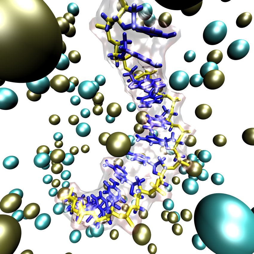
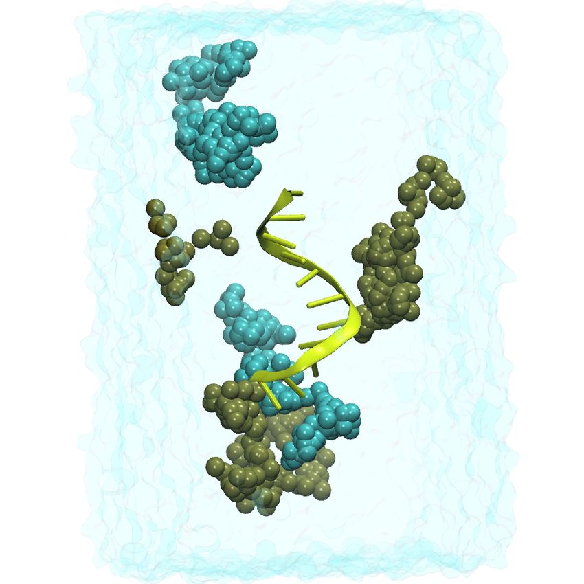
(a) Image of every tenth frame show- (b) Image of all frames showing at
ing at once, smoothed with a ten-frame once, for two Na+ ions and two Cl−
window. ions. Water is shown as a transparent
MSMS surface.
Figure 10: Two examples of showing multiple frames at once.
9 Finally, we’ll see how to make VMD “update” the selection each frame.
Hide the representation showing all frames, and reshow your first repre-
sentation, showing only DNA. Then make a new representation, with the
selection text
ions and within 5 of segname ADNA
This will show all ions within 5 Å of the DNA.
10 Now play the trajectory. (A movie of the trajectory is provided as noupdate.mpg,
and illustrated in Fig. 11.) Notice anything wrong? Although the ions
may be near the DNA for a little while, they soon wander off, and are
still shown despite no longer meeting the selection criteria. The Update
Selection Every Frame option in the Trajectory tab of the Graphical Rep-
resentations window remedies this, doing exactly what its name says. See
Fig. 12
CatDCD. On Linux/Unix systems, VMD comes with the CatDCD
program, which allows users to combine multiple trajectory files into
one, with a variety of options.2 WORKING WITH TRAJECTORIES 20
Figure 11: Movie noupdate.mpg.
Figure 12: Movie update.mpg.
You now know the basics of working with trajectories. We will next look at
some more advanced things we can do with them.
2.2 Advanced Trajectory Topic
In this section, we will explore an advanced technique for visualization. We will
look at a trajectory from a simulation in which a “virtual pore” was collapsed
around a short strand of DNA, and see how to use VMD to superimpose the
position of the virtual pore at each timestep. Along the way we will learn about
VMD’s custom graphics capabilities.2 WORKING WITH TRAJECTORIES 21
1 Start a fresh VMD session, and load the files pore.psf and pore.dcd,
and set up a representation showing just the DNA.
2 For this section, we will be examining a script. Let’s see what it does.
Type the following in the Tk Console window:
source pore.tcl
enabletrace
3 Start the animation. The blue cylinder is drawn at the radius of the
potential used in the simulation. (See Fig. 13.)
Figure 13: Movie pore.mpg.
4 Now hide your DNA representation, and type the command enablearrows.
5 Restart the animation. The DNA is now drawn by the script as well, rep-
resented as arrows. You should see something like Fig. 14. The command
disablearrows will turn this off. disabletrace will turn off everything
done by this script.
6 Now that we see what it does, let’s look at the script. Open the file
pore.tcl in a text editor.
7 The first few lines defines the procs for enabling and disabling the script:
proc enabletrace {} {
global vmd frame
trace variable vmd frame([molinfo top]) w drawcounter
}2 WORKING WITH TRAJECTORIES 22
Figure 14: DNA represented as arrows.
proc disabletrace {} {
global vmd frame
trace vdelete vmd frame([molinfo top]) w drawcounter
}
These procs use the trace feature of Tcl, which is a mechanism for setting
up some action when some variable changes. The command
trace variable vmd frame([molinfo top]) w drawcounter
says to call the command drawcounter everytime the variable vmd frame
([molinfo top]) is written (w above is short for write). See the VMD
User’s Guide at http://www.ks.uiuc.edu/Research/vmd/current/ug/ug.html
for a list of VMD variables that trace can be used with.
8 The next few lines set up the procs to turn the arrows on and off:
set pore draw arrows 0
proc enablearrows {} {
global pore draw arrows
set pore draw arrows 1
}2 WORKING WITH TRAJECTORIES 23
proc disablearrows {} {
global pore draw arrows
set pore draw arrows 0
}
9 Next we have procs which draw the arrows:
proc vmd draw arrow BASE {mol start end} {
set coneEnd [vecadd $end [vecscale 0.25 [vecsub $end $start]]]
graphics $mol cylinder $start $end radius 1.0
graphics $mol cone $end $coneEnd radius 1.5
}
proc vmd draw arrow {mol start end} {
set middle [vecadd $start [vecscale 0.8 [vecsub $end $start]]]
graphics $mol cylinder $start $middle radius 1.0
graphics $mol cone $middle $end radius 1.5
}
These simply draw the arrows by using built-in procs for drawing cylinders
and cones.
10 Next, the script sets some parameters defining the size of the pore cylinder
and how it changes through the trajectory:
set Rstart 14
set Rrate 0.00001
set Rtarget 4.0
set frameRate 10000
set Center 0.0
Obviously, these should coincide with those used in the original simulation.
11 Now we make note of the DNA residues:
set sel [atomselect top "segid ADNA and name P"]
set residList [lsort -integer [$sel get resid] ]
set residStart [lindex $residList 0]
set residEnd [lindex $residList end]
12 Now we get to the real meat of the script: the drawcounter proc. This is
the procedure called every time the frame changes.
proc drawcounter { name element op } {
...
}
trace calls the callback proc with three aruments, which are basically just
the arguments we provided trace to begin with, and which we don’t use.2 WORKING WITH TRAJECTORIES 24
Figure 15: Movie arrows.mpg.
13 Now let’s look at the drawcounter proc itself. First, it sets some global
variables, which we won’t reproduce here. Then it calculates the proper
radius of the cylinder for the current timestep:
set R [expr $Rstart - $Rrate*$frameRate \
*$vmd frame([molinfo top]) + 1.0]
if {$R < $Rtarget} {
set R $Rtarget
}
14 Next is the code which actually draws the cylinder:
draw delete all
draw color blue
draw material Transparent
set start pt [list 0 0 [expr $Center - 30]]
set stop pt [list 0 0 [expr $Center + 50]]
draw cylinder $start pt $stop pt radius $R resolution 32
Here we use VMD’s draw command to set the drawing parameters and
draw the cylinder.
15 Finally, we draw the DNA arrows, if it’s enabled:
if { $pore draw arrows } {
for {set resid [expr $residStart]} {$resid < $residEnd} {incr resid} {
set residONE [expr $resid + 1]
set tmpSel1 [atomselect top "resid $resid and name N1 C3’"
frame $vmd frame([molinfo top])]
foreach {coordN1 coordC1} [$tmpSel1 get "x y z"] { break }2 WORKING WITH TRAJECTORIES 25
draw color yellow
vmd draw arrow BASE top $coordC1 $coordN1
set tmpSel2 [atomselect top "(resid $resid and name P)
or (resid $residONE and name P)" frame $vmd frame([molinfo top])]
foreach {coordP1 coordP2} [$tmpSel2 get "x y z"] { break }
draw color 14
vmd draw arrow top $coordP1 $coordP2
$tmpSel1 delete
$tmpSel2 delete
}
}
The script simply uses the atomic coordinates of three of the atoms of
each base to define where the arrow should be drawn, then the appropriate
drawing command, defined above, is called.
You now have some powerful techniques for working with trajectories. The last
section of this tutorial will show you how to take everything you’ve learned to
produce movies of your system.
2.3 Making Movies
In this final section, you’ll first learn how to make a basic movie. Then we’ll see
how to do more advanced animations, again using Tcl’s callback functionality.
1 Leave everything loaded in VMD from the last section, or start a fresh
VMD session and type source makingmovies-restart.tcl in the Tk
Console window to load everything you need for this section. To make
our movies, we will use the VMD Movie Maker plugin. Go to Extensions
→ Visualization → Movie Maker.
2 First, let’s look at some of the options for our movie. Click on the Movie
Settings menu. In additon to a trajectory movie, Movie Maker can also
take still frames and animate camera motion.
3 Set up your representations and angle to something you like.
4 Select Rock and Roll, set the working directory to something convenient,
give your movie a name, and click Make Movie. You will see the VMD
display update as the movie is made.
5 Once VMD is finished, open the movie. This movie setting is good for
showing one side of your system primarily.
6 Now, try a trajectory movie. Select Movie Settings → Trajectory, give this
one a different name, and click Make Movie.2 WORKING WITH TRAJECTORIES 26
Renderers. For better-looking movies, try the different rendering
options in the Renderer menu.
7 It is possible to show multiple views of your molecule at once, which can be
very helpful in some cases. Load the files pore.psf and pore.dcd again,
creating a new molecule. (You may want to rename it by double-clicking
its name.)
8 Fix the original molecule by double-clicking the “F” next to its name in
the VMD Main window. Now you can manipulate the view of the second
copy without affecting the first. Make your window wider, and use the
Translate mouse mode to shift your second view to the left of the first.
Figure 16: Movie 2views.mpg.
9 Since the new copy is its own molecule, you have complete control of
how it is displayed, independent of the original copy. When you play the
trajectory or make a movie, VMD will keep the two views synchronized.
The file 2views.mpg shows an example of this technique, as does Fig. 17.
10 Finally, we’ll look at how to use user-defined scripts to dictate the anima-
tion. Type the following commands in the Tk Console:
source usermovie.tcl
enablemoviecallback
Now select Movie Settings → User Defined Procedure, and click Make Movie.
Now, in addition to simply going through the trajectory, the camera starts
above the DNA and rotates down and around it. An example movie is
provided, and shown in Fig. 182 WORKING WITH TRAJECTORIES 27
Figure 17: Example of showing the same object from multiple perspectives.
Figure 18: Movie usermovie.mpg
11 Let’s see how it works. Its contents are reproduced here:
set trajectory frames [molinfo top get numframes]
proc moviecallback { args } {
global trajectory frames
set frac [expr double($::MovieMaker::userframe)/$::MovieMaker::numframes]
rotate z to [expr $frac*360.0]
rotate x by [expr -90.0*$frac]
set frac [expr double($::MovieMaker::userframe)/$::MovieMaker::numframes]
animate goto [expr $frac * $trajectory frames]
}2 WORKING WITH TRAJECTORIES 28
proc enablemoviecallback { } {
animate goto 0
trace add variable ::MovieMaker::userframe write moviecallback
}
proc disablemoviecallback { } {
trace remove variable ::MovieMaker::userframe write moviecallback
}
This should look familiar. We are again using the trace feature of Tcl.
The Movie Maker plugin sets the writes the variable ::MovieMaker::userframe
each time it changes frames for animation, and when that happens, our
proc moviecallback is called. This proc rotates the scene, and advances
the animation frame.
You’ve now completed the tutorial. We’ve seen a number of techniques for
representing molecular systems clearly and effectively, and gotten a taste of
VMD’s capabilities. The VMD website, listed at the beginning of this tutorial,
has many other tutorials and resources for VMD users.
Acknowledgements
Development of this tutorial was supported by the National Institutes of Health
(P41-RR005969 - Resource for Macromolecular Modeling and Bioinformatics)You can also read