Void content computation using optical microscopy for carbon fiber composites
←
→
Page content transcription
If your browser does not render page correctly, please read the page content below
DEGREE PROJECT IN THE FIELD OF TECHNOLOGY
MATERIALS DESIGN AND ENGINEERING
AND THE MAIN FIELD OF STUDY
MATERIALS SCIENCE AND ENGINEERING,
SECOND CYCLE, 30 CREDITS
STOCKHOLM, SWEDEN 2020

Void content computation using
optical microscopy for carbon
fiber composites

FANNI, SAMAN

KTH ROYAL INSTITUTE OF TECHNOLOGY
SCHOOL OF ENGINEERING SCIENCES
Void content computation using
optical microscopy for carbon fiber
            composites

                   Fanni, Saman

    SE202X Degree Project in Solid Mechanics, Second Cycle
               KTH School of Engineering Sciences
              Department of Engineering Mechanics
                 Lightweight Structures Division
                   SE-100 44 STOCKHOLM

SE202X Degree Project in Solid
                      Mechanics, Second Cycle

                  Void content computation using
                 optical microscopy for carbon fiber
                             composites

                                   Saman Fanni
Approved       Examiner                  Supervisor(s)
2020-10-16     Bo Alfredsson             Sara Eliasson
                                         Per Wennhage
                                         Zuheir Barsoum
Commissioner   Contact Person(s)
Scania CV AB   Saman Fanni, Sara Eliasson, Per Wennhage,
               Zuheir Barsoum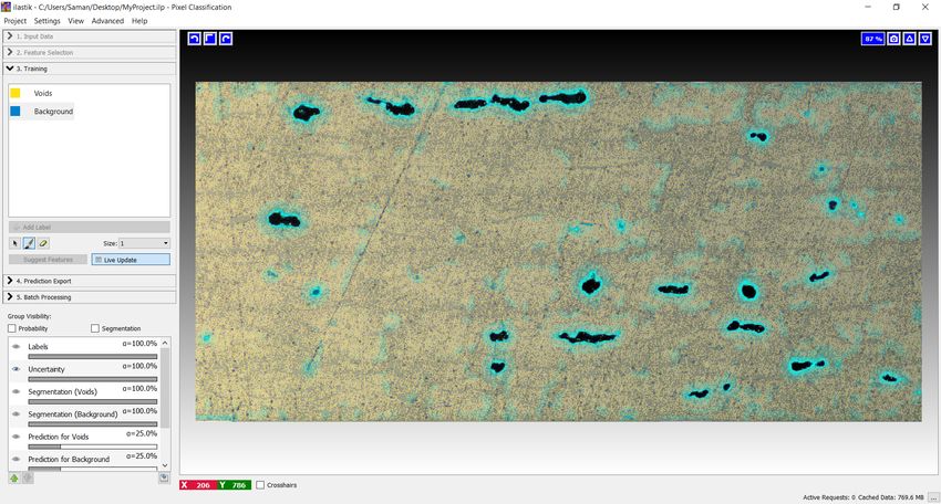
SE202X Examensarbete inom
                   Hållfasthetslära, avancerad nivå

                    Beräkning av kavitetshalter för
                    kolfiberkompositer med optisk
                              mikroskopi

                                   Saman Fanni
Godkänd        Examinator                Handledare
2020-10-16     Bo Alfredsson             Sara Eliasson
                                         Per Wennhage
                                         Zuheir Barsoum
Beställare     Kontaktperson(er)
Scania CV AB   Saman Fanni, Sara Eliasson, Per Wennhage,
               Zuheir Barsoum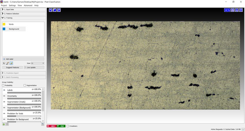
Abstract
Three different void content calculation techniques using optical microscopy were
compared in multiple-user trials. The three methods studied comprised of a selection,
thresholding, and semi-automatic machine learning method. The techniques were
applied to micrographs of three carbon fiber-epoxy composite plates manufactured
in-house, where one plate had reduced void content by means of debulking prior
to curing. The users performed the techniques on the sets of micrographs and the
standard deviation between the users void content results were measured. The
advantages of the three methods were discussed and their practical applications were
proposed.

The trials showed agreement between users on what are voids and not as well as
showing that uncertainties in void content are specimen-specific and not attributed to
different users or methods applied. All three methods showed satisfying precision in
calculating void content compared to void content quality levels provided by literature.
It was found that thresholding, which is the current standard method of void content
calculation using microscopy, inhabits an unscientific bias which compromises the le-
gitimacy of the method. The study formulates a manual selection-based method using
edge-detection selection tools intended to benchmark void content in images, as well
as proposing a route to the automation of void content analysis using microscopy.

Sammanfattning
Tre olika beräkningstekniker för kavitetshalter med hjälp av mikroskopi jämfördes
genom fleranvändar-tester. De tre metoderna innefattade en selektions-metod,
tröskelvärdesmetod, och en övervakad maskininlärningsmetod. Metoderna applicer-
ades på mikrografer av tre kolfiber-epoxi kompositplattor tillverkade internt, varav en
platta hade reducerad kavitetshalt genom en avbulkningsprocess innan härdning.
Användarna genomförde metoderna på mikrograferna och standardavvikelsen mellan
användarnas resulterande kavitetshalter mättes. För- och nackdelarna hos de tre
metoderna diskuterades och deras praktiska applikationer föreslogs.

Testerna visade en överensstämmelse mellan användare om vad som omfattar
kaviteter och inte, samt en påvisning på att osäkerheter kring kavitetshalter är
provbitberoende och inte användar- eller metodberoende. Alla tre metoder uppvisade
en tillfredsställande precision i kavitethaltsberäkning jämfört med kvalitetsnivåer av
kavitethalter erhållna från litteratur. Det konstaterades att tröskelvärdesmetoden, vilket
är nuvarande standardmetoden för kavitethaltsberäkning med mikroskopi, innehar en
bias som sätter validiteten av metoden i fråga. Studien formulerar även en manuell
selektions-metod som använder selektions-verktyg för randdetektering, ämnad för att
hitta referensvärden för kavitetshalter. Förslag ges även kring tillvägagångssättet till
att uppnå automatiserade metoder för kavitethaltsberäkning.

                                            ii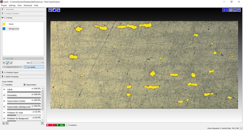
Foreword
This work was conducted at the Royal Institute of Technology, Centre for ECO2 Vehicle
Design on behalf of Scania CV AB. The work was part of a larger research project on
fatigue and void culture on fiber-reinforced plastics (FRPs).
Contents
Abstract                                                                                                                            i

Foreword                                                                                                                           iii

1 Introduction                                                                                                                      1

2 Literature review                                                                                                                 2
  2.1 Carbon fiber reinforced plastics (CFRP) . . . . . . . .                          .   .   .   .   .   .   .   .   .   .   .    2
  2.2 Void formation . . . . . . . . . . . . . . . . . . . . .                         .   .   .   .   .   .   .   .   .   .   .    3
       2.2.1 “Snap cure” epoxy resin . . . . . . . . . . . .                           .   .   .   .   .   .   .   .   .   .   .    4
  2.3 Effect of voids on the mechanical properties of FRPs .                           .   .   .   .   .   .   .   .   .   .   .    4
       2.3.1 Tensile properties . . . . . . . . . . . . . . . .                        .   .   .   .   .   .   .   .   .   .   .    5
       2.3.2 Compressive properties . . . . . . . . . . . .                            .   .   .   .   .   .   .   .   .   .   .    5
       2.3.3 Interlaminar shear properties . . . . . . . . .                           .   .   .   .   .   .   .   .   .   .   .    5
       2.3.4 Fatigue properties . . . . . . . . . . . . . . .                          .   .   .   .   .   .   .   .   .   .   .    6
  2.4 Void characterization techniques . . . . . . . . . . .                           .   .   .   .   .   .   .   .   .   .   .    7
       2.4.1 Density measurement . . . . . . . . . . . . .                             .   .   .   .   .   .   .   .   .   .   .    7
       2.4.2 Microscopy . . . . . . . . . . . . . . . . . . .                          .   .   .   .   .   .   .   .   .   .   .    8
       2.4.3 Ultrasonic testing . . . . . . . . . . . . . . . .                        .   .   .   .   .   .   .   .   .   .   .   11
       2.4.4 Radiographic methods . . . . . . . . . . . . .                            .   .   .   .   .   .   .   .   .   .   .   12

3 Methods                                                                                                                          13
  3.1 Material characteristics . . . . . . .   .   .   .   .   .   .   .   .   .   .   .   .   .   .   .   .   .   .   .   .   .   13
  3.2 Specimen preparation . . . . . . .       .   .   .   .   .   .   .   .   .   .   .   .   .   .   .   .   .   .   .   .   .   13
  3.3 Void content computation methods         .   .   .   .   .   .   .   .   .   .   .   .   .   .   .   .   .   .   .   .   .   14
      3.3.1 Selection-method . . . . . .       .   .   .   .   .   .   .   .   .   .   .   .   .   .   .   .   .   .   .   .   .   14
      3.3.2 Thresholding . . . . . . . .       .   .   .   .   .   .   .   .   .   .   .   .   .   .   .   .   .   .   .   .   .   15
      3.3.3 Machine learning-method .          .   .   .   .   .   .   .   .   .   .   .   .   .   .   .   .   .   .   .   .   .   17
  3.4 Multiple-user trials . . . . . . . . .   .   .   .   .   .   .   .   .   .   .   .   .   .   .   .   .   .   .   .   .   .   18
      3.4.1 Trial 1 . . . . . . . . . . . .    .   .   .   .   .   .   .   .   .   .   .   .   .   .   .   .   .   .   .   .   .   18
      3.4.2 Trial 2 . . . . . . . . . . . .    .   .   .   .   .   .   .   .   .   .   .   .   .   .   .   .   .   .   .   .   .   18

4 Results                                                                                                                          19
  4.1 Trial 1 . . . . . . . . . . . . . . . . . . . . . . . .                  .   .   .   .   .   .   .   .   .   .   .   .   .   19
  4.2 Trial 2 . . . . . . . . . . . . . . . . . . . . . . . .                  .   .   .   .   .   .   .   .   .   .   .   .   .   20
  4.3 Evaluation of void characteristics between plates                        .   .   .   .   .   .   .   .   .   .   .   .   .   23
  4.4 Final determination of total plate void content . .                      .   .   .   .   .   .   .   .   .   .   .   .   .   23

5 Discussion                                                                                                                       23
  5.1 Discussion of graphs and results . . . . . . . . . . .                       .   .   .   .   .   .   .   .   .   .   .   .   23
       5.1.1 Void content deviation effect on fatigue life                         .   .   .   .   .   .   .   .   .   .   .   .   25
  5.2 Comparison of the computation methods . . . . . .                            .   .   .   .   .   .   .   .   .   .   .   .   25
       5.2.1 Sensitivities and precision . . . . . . . . . .                       .   .   .   .   .   .   .   .   .   .   .   .   26
       5.2.2 When to use each method . . . . . . . . . .                           .   .   .   .   .   .   .   .   .   .   .   .   28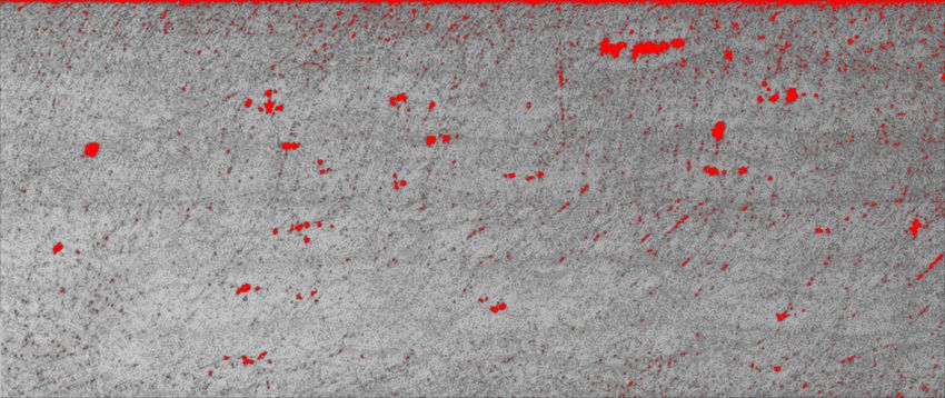
6 Conclusions                                                                         29

7 Future work and recommendations                                                     30

Acknowledgements                                                                      31

List of Figures                                                                       33

List of Tables                                                                        34

List of abbreviations and symbols                                                     35

References                                                                            36

Appendix A Trial results tables                                                       40

Appendix B Instructions for void content computation methods                          43
  B.1 Selection-method with Adobe® Photoshop® /Affinity® Photo . . . . . . .          43
  B.2 Thresholding with Fiji/ImageJ . . . . . . . . . . . . . . . . . . . . . . . .   44
  B.3 Machine Learning-method with ilastik and Fiji . . . . . . . . . . . . . . .     45

Appendix C Fiji macro for a more automated thresholding method                        50

Appendix D Fiji macro for void content calculation on ilastik-exported images 51

Appendix E Manufacturing details of CFRP plates                                       53

Appendix F Specimen preparation details                                               54
1    Introduction
Fiber composite materials are becoming much more frequently used by the vehicle and
transportation industry as they are corrosion resistant, can be tailored to fit specific
purposes, but foremost, for their high strength-to-weight ratio or “specific strength”.
With rising greenhouse emissions it is vital to find lighter materials to replace the
mainly metal components in today’s vehicles as it would increase energy efficiency.
Materials with high specific strength are distinctively suited for this advancement.

Although fiber composite materials allow lighter components to be made, they are
primarily made with a liquid resin matrix which after solidifying retains an amount
of gas bubbles within the material, creating porous inclusions or voids. These void
defects can act as failure initiation points, causing either delamination, where the
void weakens the bonding between laminae causing detachment, or matrix cracking,
where a crack propagation from the matrix through the material can cause a sudden
catastrophic failure [1]. Composite materials are greatly affected by voids due to their
usually brittle behaviour. Especially fatigue life and damage propagation are affected,
more so than static loading capacity or any other failure mechanism [1, 2]. Fatigue life
and damage propagation are detrimental in the reliability of a structural component
and are usually the culprits behind most of society’s mechanical failures [3]. Hence,
engineers commonly design their components to withstand a fatigue failure as it is the
dimensioning factor.

In summary, voids and pores can heavily reduce the strength and reliability of a fiber
composite structure. As such, the reduction of voids is detrimental to the reliability
of composite structures and a vital aspect when manufacturing fiber composites. The
methods of finding, studying and characterizing voids and pores in a fiber composite
are however not as well established and the different methods currently available have
different benefits and drawbacks.

A commonly used method for studying the insides of materials, microscopy, is preva-
lently used for void characterization. The process of taking images of cross-sections
inside the material is generally known to most practitioners of microscopy; the process
of calculating void content from these images is however not well-established. The
actual method of calculation itself is often left to the user, meaning uncertainties might
occur around the results depending on the user and method used.

This study aims to investigate in greater detail the practical side of void content com-
putation using microscopy. Carbon-fiber epoxy plates were manufactured in-house and
microscopic images were taken of cross-sections and prepared for void content com-
putation. Three void content computation methods using different approaches were
established and performed in multiple-user trials. The multiple-user trials examined
numerous aspects of each method: reproducibility of results between different users us-
ing the same method, consistency of results between different methods on same images,
ease of use for common users and lastly time-efficiency. The ambition was to find possi-
ble pitfalls, inconsistencies and deficiencies with the available void content computation
methods and propose suitable applications for each method.
                                            1
2 Literature review
2.1 Carbon fiber reinforced plastics (CFRP)
A composite material is a material made from two or more constituent materials that
when combined produce a material with characteristics different from the individual
constituents. Usually, composite materials inhibit higher specific strength and specific
stiffness than their constituent materials and are used for this purpose. Examples of
composite materials include steel-reinforced concrete, reinforced plastics such as fiber-
glass, wood composites such as plywood, composite glass, or the most used material
in the world, concrete. The different types of composites include particle-reinforced,
fiber-reinforced, and structural composites, illustrated in Figure 1. Particle- or fiber-
reinforced composites consist of two phases: matrix and reinforcement. The matrix
material binds to the reinforcement, maintaining its desired position and orientation,
protecting it from environmental damages and acting as a load transfer medium.
Meanwhile, the reinforcement increases the load-bearing capacity of the matrix and
is the main load-carrying constituent. Technologically, fiber-reinforced composites are
the most influential and effective type of composite due in part to the lack of defects
present in the thin fibers, giving them higher strength and stiffness than their precursor
bulk materials [1, 4].
Figure 1: A hierarchic schematic of different classes of composites [4].
Carbon fiber-reinforced plastics (CFRP) is a fiber-reinforced composite with a plastic as
the matrix phase and carbon fiber as the reinforcement phase. Epoxy is a commonly
used matrix material in CFRP composites due to its high strength and stiffness. Since
fibers only provide strength in the direction of the fiber length, layers of carbon fiber
are stacked with different orientations on top of each other, creating a laminate better
suited for various loadcases.
22.2 Void formation
Ideally, a composite would solely consist of fiber and matrix. In reality, manufacturing
defects such as voids and volatiles are a part of the volume of the composite and are
difficult to limit. The volume contents of the composite can be described by Equation 1
and 2, where Vf denotes the fiber volume fraction, Vm the matrix volume fraction, and
Vv the void volume fraction. Equation 1 describes the ideal composite volume fractions
and Equation 2 describes the true volume fractions.
Vf + Vm = 1 (1)
Vf + Vm + Vv = 1 (2)
The presence of voids can be traced to multiple sources: volatiles in the resin system,
moisture dissolved in the resin, mechanical air entrapment during stacking, mechanical
air entrapment between tows during impregnation, and fabrication mishaps such as a
leaking vacuum bag or pump [5]. Combined, these sources lead to two types of voids:
intra-laminar voids and inter-laminar voids. As their names suggests, the voids are
either present inside of a lamina or fiber tow, or between laminae [6], illustrated in
Figure 2.
Figure 2: An illustration of a composite with an inter- and intra-laminar void.
Void formation differ between manufacturing methods of composites. This is due to
the thermodynamic and rheological properties of the matrix material and how the man-
ufacturing process combines the constituent materials together. In Liquid Composite
Molding (LCM), a method including common manufacturing methods such as Vacuum-
Assisted Resin Transfer Method (VARTM) or Resin Transfer Molding (RTM), the matrix
3material is infused into a preform containing the reinforcement. The void formation
during these manufacturing methods differ from those using prepreg fiber sheets, where
the fibers have been impregnated with the matrix in advance. For prepregs, the main
sources of voids are the intra-laminar voids occuring during impregnation and inter-
laminar voids caused by air entrapment during stacking. During impregnation, the air
inside tows are challenging to remove since a viscous resin has only difficulty penetrat-
ing through tightly packed bundles of fibers, especially if the fibers have low wetability.
Earlier prepreg generations consisted of resins containing higher amounts of volatiles
leading to increased void content from this source type, something modern prepreg
sheets encounter less [6, 7]. Although difficult, for both prepreg and LCM manufactur-
ing methods, void content can be controlled by changing parameters such as pressure,
temperature, resin viscosity and curing time [8].
2.2.1 “Snap cure” epoxy resin
The curing time for fiber composites can be too lengthy for a cost-effective production
cycle. To permit a time- and cost-efficient production cycle, manufacturers have
developed resin systems able to cure in a few minutes. These types of resin systems are
commonly called “snap cure”. Snap cure epoxy resins are developed to enable rapid
manufacturing processes suitable for industries such as the vehicle industry. They are
designed to sustain a longer shelf life in room-temperature and to be made rapidly
by hot compression molding, a process commonly used in rapid manufacturing, with
curing times around 2-4 minutes [9, 10].
Due to the short cure time and low cure temperature needed for snap cure resins, air
bubbles will have a harder time migrating out of the resin due to the higher resin vis-
cosity and shorter migration time.
2.3 Effect of voids on the mechanical properties of FRPs
It is widely known that voids reduce the mechanical properties of fiber composites and
is the reason why voids are generally studied. Engineers have tried estimating the effect
of voids on structural reliability and strength, but these “rule-of-thumbs” are deemed
insufficient and inaccurate [11]. Purslow [12] proposed a chart shown in Table 1 as a
means of estimating the quality and performance of a composite containing a certain
void content level. The chart shows how a difference of just a few fractions of a percent
in void content can lead to a large difference in quality, compared to the much larger
50-70% levels of fiber and matrix contents.
An extensive number of studies have been performed investigating the effect of voids on
fiber composites trying to quantify the relationship between the two. With countless dif-
ferent combinations between material properties to investigate, load cases, constituent
materials and stacking sequences, there are plentiful relationships to be investigated. It
is therefore important to choose material properties, materials and stacking sequences
that are widely used for structures that require high quality and load cases most de-
manding for fiber composites, when choosing what to investigate.
4Table 1: Purslow’s [12] composite quality chart depending on void volume
content Vv .
Grade A Vv ≤ 0.2% Excellent
Grade B 0.2% < Vv ≤ 0.5% Very good
Grade C 0.5% < Vv ≤ 1% Good
Grade D 1% < Vv ≤ 2% Fair
Grade E 2% < Vv ≤ 5% Poor
Grade F 5% < Vv Very poor
2.3.1 Tensile properties
The effect of voids on tensile properties can be summarized with either a modulus or
strength reduction. For both properties, authors have reported similar effect with an
increase of voidage. Sisodia et al. [2] investigated the effect of voids on the quasi-static
behaviour of carbon-epoxy composites. They found a negligible effect of voids on the
static tensile properties of the composites and recommended not to assess the strength
of composites affected by voidage with static testing. Huang and Talreja [8] investigated
the effect of voids on the tensile modulus properties of fiber composites and found with
a void content increase of 1%, the longitudinal and transverse elastic moduli Ex and Ey
decreased proportionally with 1%, while the out-of-plane modulus Ez decreased with
between 4-7%. The out-of-plane sensitivity was thought to be due to voids at the ply
interface region.
2.3.2 Compressive properties
The compressive properties of fiber composites are not as widely studied as tensile
properties, as suggested by a reviewal study [7], even though there is consensus that
composites containing voids are more sensitive to compression than tension. Authors
have found a decrease of 3-7% in failure stress during compression with a void content
increase of 1% and a similar relationship with compression modulus [13].
2.3.3 Interlaminar shear properties
The interlaminar region of FRPs are weaker than the intralaminar region due to a lesser
presence of fibers. This interface is dominated by the properties of the matrix and since
voids greatly affect the usually weaker and brittle matrix, interlaminar shear strength
(ILSS) is one of the most studied properties linked to voids. In a literature review, Judd
and Wright [6] found an approximate decrease in ILSS of 7% for a 1% increase in void
content for void contents between 0-4%. They found the relationship to exist regardless
of resin, fiber or fiber surface treatment used in the manufacturing process. Hence
showing how important it is to aim for essentially void-free composites for high-load
bearing structures. In an experimental study, Ghiorse [5] found a decrease of 10% in
5ILSS for each 1% increase in void content for void contents between 0-5%, higher than
that found by Judd and Wright [6]. Similarly, it was concluded that this relationship
likely exists regardless of constituent materials.
2.3.4 Fatigue properties
Fatigue is a form of failure that occurs in structures subjected to cyclic or dynamic
loading. Structural components usually undergo this type of fluctuating load pattern
during their service lives, especially fiber composites since they are used mainly for
their stiffness and load-bearing capacities. An experimental fatigue study can be
arduous. In addition to choice of materials and stacking sequence, aspects such as load
frequency, load level, load direction and load ratio must be chosen carefully just for
the purpose of the test itself leading to a variety of combinations in literature. Albeit,
many studies have been performed on the effect of defects on fatigue resistance of
composites. Sisodia et al. [2] tested porous carbon fiber composites under both static
and fatigue loading. They recorded a significant drop in fatigue life with increased
void content compared to a negligible drop in static strength. With an increase of void
content from 1% to 2%, fatigue life is reduced with 77%. From their study, Figure 3
shows a comparison between static and fatigue strength as a function of void content.
(a) (b)
Figure 3: a) Normalised engineering properties as a function of void content
taken from Sisodia et al. [2]. b) Adapted version of the same chart displaying
the fatigue life reduction of 77% for a void content increase from 1% to 2%.
Maragoni et al. [14] studied the fatigue behaviour of glass-fiber composites under the
presence of voids. They reported a significant effect of voids on both fatigue life and
crack growth rate. Fatigue life was reduced by 80% for a void content of 0.34% on
a cross-ply laminate compared to a void-free one, and with 65% for a void content of
61.07% on an angle-ply laminate compared to the void-free one. Lambert et al. [15]
however did not find a reduction in fatigue life with higher void content, void spatial
distribution or average void size on their study on glass-fiber composites. Instead, a cor-
relation between reduced fatigue life and the size of the largest single void was found,
although below their 95% statistical confidence level. However, accounting for the void
location in the composite, void size in conjunction with critical locations showed a cor-
relation above the confidence level. These two studies [14,15] discussed the convention
of using void content as a form of structural reliability assessment. They proposed to
not only use void content but other void characteristics as well such as void size, spatial
distribution and location in a combined and improved assessment model.
2.4 Void characterization techniques
Many different void characterization methods are available with each having distinct
advantages and purposes. Void characteristics such as void content, size, shape (mor-
phology), location and spatial distribution are possible to obtain through the most com-
mon methods. Characteristics such as void size can occasionally be obtained through
the inherent software of the digital microscope, and void location is obtainable simply
by observing the micrograph. Following is a review of the most common void charac-
terization methods and their uses.
2.4.1 Density measurement
The void content can be obtained by measuring the density of the fibers and the resin
separately. Together with their weight fractions of the composite, this would yield a
theoretical density which can be compared to the actual density of the composite. The
theoretical density should theoretically only contain the fibers and the resin with no
void inclusions. In actuality, voids are presumably present. Since voids add volume but
not mass, the presence of voids will decrease density. Therefore, the difference between
the theoretical and measured density of the composite is the void content in volume
fraction. Described in ASTM D2734 [16], the void content can then be computed with
the following equation:
T
ρc − ρM
WR Wf c
ρTc = 100 + , Vv = 100 (3)
ρR ρf ρTc
or with a simplified version where the theoretical density is not directly computed:
WR Wf
Vv = 100 − ρM
c + (4)
ρR ρf
7where ρTc denotes the theoretical density of the composite, WR the resin weight
percentage, Wf the fiber reinforcement weight percentage, ρR the density of the resin,
ρf the density of the reinforcement, ρM
c the measured density of the composite, and Vv
the void content.
The densities of the resin and composite can be measured using Archimedes’ principle
of water buoyancy, described in ASTM D792, or by observing the level of which the
material sinks in a column of water, called the density-gradient technique, described
in ASTM D1505 [16–18]. However, the density of the fiber reinforcement should be
measured using Archimedes’ principle [7]. The weight fractions of the fiber reinforce-
ment and resin can also be done in primarily two ways, namely matrix burn-off (matrix
ignition) or matrix digestion. Matrix burn-off utilizes heat to burn away the resin, while
matrix digestion dissolves the resin matrix using acids, described in ASTM D2584 and
ASTM D3171 respectively [19, 20]. The weight of the specimen is measured before and
after removal of the resin, and the weight fraction can be determined. Matrix digestion
may produce toxic fumes during its process, making the method possibly dangerous
compared to matrix burn-off.
The density measurement method does bring some complication of errors. It is assumed
that the resin density by itself is the same as the resin density when in a composite. Re-
ally, the density of a resin can differ when in bulk compared to when constituting a
composite material, generally being lower when in bulk. This can be caused by differ-
ences in curing, heat, pressure, and the presence of boundary forces between fiber and
resin when manufacturing a composite [16]. The density measurement method also
requires high accuracy in its measurements and has a tendency to report negative void
content values which is a theoretical impossibility [21, 22]. It is estimated that its void
content accuracy lies around 0.5% [7]. Although being a destructive technique with
relatively low accuracy it can process large amounts of samples rapidly.
2.4.2 Microscopy
Also a destructive technique, microscopy uses optical or electron microscopy images
(micrographs) of cross sections from specimens to determine void characteristics.
Aside from void content, microscopy also allows the evaluation of void size, shape,
location and spatial distribution. Regarding calculating void content, various types
of image analysis methods are available. One such method, the “optical counting
technique”, uses probability to quickly estimate void content. By applying a regular
square grid pattern over the micrograph image, the void content can be estimated by
counting the fraction of the squares whose centers lies over a void. By probability,
that fraction should equal the void content. Possibly the quickest method of all
is the “optical comparison technique”. It estimates the void content by comparing
micrographs with catalogued figures or illustrations of other micrographs whose void
content is known; so a visual estimation can be done extremely quickly compared to
any other method [12]. The “area fraction” method, an intuitive approach, calculates
the void content by determining the area fraction of the micrograph that consists of
voids. This requires accuracy in the area calculation of the usually complex-shaped
8voids. Similar to the optical counting technique, void spatial distribution can be
assessed using the “local mapping technique”. By applying a square grid pattern
over the micrograph, the number and area fraction of voids in each square can be
counted, visualizing the void spatial distribution. This is nonetheless only a qualitative
and estimative evaluation of spatial distribution, whereas quantitative methods are
more useful [23, 24]. Fortunately, with the help of digital image processing tools
the calculation of void characteristics is quick and requires little effort, making the
estimative methods obsolete.
Calculating void characteristics in a micrograph imposes some obstacles which could
compromise repeatability and accuracy. A standardized method or software is still
nonexistent for microscopic void characterization and choice of method is often left
to the investigator or is a laboratory specific convention. In this section, different
softwares and image analysis techniques for void characterization are explored.
Raster graphics editors
These types of software allow users to create and manipulate pixel images, also called
“raster” images. Examples of raster graphics editors include, but is not limited to,
Adobe® Photoshop® software, Affinity® Photo, or GIMP© open-source image editor.
For void characterization it is especially useful to isolate and/or count specific pixels,
cut and trim the image, or adjust the colors of the image for improved visualization.
With raster graphics editors it is possible to calculate the void content of a micrograph
in a highly controlled fashion.
Image processing programs
Similar to raster graphics editors, image processing programs offer equivalent tools
but are created specifically for scientific image analysis. Although the number of
tools offered are fewer than in raster graphics editors, the tools in image processing
programs are selected for their convenience in image analysis and they offer many more
analytical tools. Most common image processing programs are free to use. Examples
of these include ImageJ, Fiji, Microscopy Image Browser, IrfanView, CellProfiler, and
ilastik. ImageJ is an open-source software developed at the National Institute of Health
and is the platform which other softwares such as Fiji is based on [25, 26]. Since it is
free and open-source, many researchers in the scientific community develop plugins
that add further tools to ImageJ. Fiji, which is an abbreviation for “Fiji Is Just ImageJ”,
is a software which is ImageJ but with several added plugins and features, revising
many deficiencies of ImageJ. Since Fiji is developed by the research community itself
and encases ImageJ, the community recommends the use of Fiji over ImageJ or other
image processing programs [26, 27]. With image processing tools it is possible to
calculate the void content as well as quantifying void shape, for example mean radius
calculation or circularity among others.
Cluster algorithms
In computer science, clustering is when a set of data points or objects are grouped into
clusters based on similar attributes they share; objects within a cluster are more similar
to each other than objects outside the cluster [28]. Applying this to void characteri-
9zation, a cluster algorithm can search an image for patterns and group together areas
that look like voids, since they have similar appearance. With all the void-looking areas
in one single group, the total void content can be calculated. Because objects can be
similar or dissimilar depending on the property being measured and because the notion
of a “cluster” is not well-defined, there are a large variety of clustering algorithms
with different approaches on how to find patterns in data sets [29]. Examples of
cluster algorithms suitable for image analysis are K-means clustering, Fuzzy C-means,
DBSCAN (Density-based spatial clustering of applications with noise), and Affinity
Propagation (not related to Affinity® graphics softwares). Each of these have distinct
advantages, and the choice of algorithm can be difficult to make [30]. For example,
K-means has a low calculation time and is simple to apply, but requires the number
of clusters as an initial input [31]. Fuzzy C-means is similar to K-means but is a
“soft” algorithm, meaning objects are assigned probabilities to whether they belong
to a cluster instead of strictly belonging to a cluster or not. Fuzzy C-means has been
shown to perform better at image segmentation than K-means [32]. DBSCAN does not
require the selection of cluster quantity and has high performance in images with a
high level of noise, but can perform inadequately in images with clusters where clusters
consist of many different colors [33]. Therefore, the choice of cluster algorithm must
take into account the underlying principles of calculation [29]. Additionally, machine
learning can be applied to algorithms by letting users annotate pixels or objects before
segmentation is performed by the program. With this approach, it is possible to
employ many different image processing algorithms in conjunction with initial user
supervision to produce more accurate results. There are a considerable amount of free
open-source machine learning programs available. Examples of these include ilastik,
Weka, TensorFlow and Google AI. With cluster algorithms and machine learning it
is possible to calculate void content and facilitate higher levels of automated calculation.
Tessellation
Lastly, in order to calculate void spatial distribution, another type of algorithm is avail-
able called “Tessellation”. In a plane containing points, tessellation involves partitioning
the plane around each point, called “sites”, into polygonal cells such that every point
inside each cell is closer to its own site than to any other site [23, 24, 34]. The subse-
quent cell diagram is called a Voronoi diagram. In Figure 4, the sequence of tessellation
is shown. Figure 4a shows a plane containing 7 sites. In Figure 4b the plane is parti-
tioned into a Voronoi diagram. Figure 4c illustrates a greyed cell as an example, where
any point within the grey area is closer to the red site within the cell than any of the
other sites. In the Voronoi diagram, each border in a cell indicates a nearest neighbor of
that cell’s site. The distance between each site and their nearest neighbors can then be
calculated. The variance of this distance describes how homogeneous the distribution
of the sites are. However, in void characterization, this distance should not be from
the centroid of the void, as it would not consider void area. The consequence of doing
so would mean voids with low circularity, especially larger ones, could neighbor other
voids closely but still have a large distance between them according to the diagram;
thus showing a higher homogeneity. Rather, the Voronoi diagram and the distances
between the nearest neighbors should be calculated from the edges of the sites.
10(a) (b) (c)
Figure 4: Illustration of a Voronoi diagram. a) Plane with 7 sites. b) Corre-
sponding Voronoi diagram of the plane. c) The grey cell consists of all points
closer to the red site than to any other site. Adapted image from [35].
In summary, microscopy is a relatively quick and simple void characterization technique
which can evaluate several void characteristics with minimal cost and user training.
It does however bring inherent errors. Microscopy is heavily section-biased, meaning
the results depend on the direction of the image section chosen for analysis [36, 37].
It is simultaneously location-biased, meaning the technique only analyzes the location
on the material in which the section is situated. This is detrimental in cases where
material properties vary depending on location. It is therefore critical and customary
that several micrographs are attained with a range of locations and sections to minimize
these biases. Around 20-25 images are recommended to reduce void content error and
provide statistically representative data [38].
2.4.3 Ultrasonic testing
Unlike density measurement and microscopy, ultrasonic testing is a non-destructive
technique (NDT), meaning it does not require the destruction of the test piece to
evaluate void characteristics. Ultrasonic testing uses high frequency sound waves to
detect the thickness of a material or potential defects within. The testing requires a
transducer, receiver, display unit and a couplant. Ultrasonic pulses are sent by the
transducer through the material while the receiving of the pulse can be done in two
ways: attenuation or reflection. With attenuation, the receiver picks up the pulse on a
different surface than the transducer, usually on the opposite side. By measuring the
amount of the pulse transmitted versus the amount received, the presence of voids can
be detected since sound intensity is greatly diminished by voids. Attenuation does not
however offer any additional information about voids. With reflection, the transducer
also receives the pulse as the sound reflects from the back wall of the material or
from imperfections within. The display unit will then show the signal transmitted and
received with their corresponding amplitude and time intervals. Some display units
may even produce images through the thickness of the material, offering information
about defect size and shape. If the velocity of sound in the material is known, the
location of the void can be determined from the time difference of the front surface
and defect reflections [39, 40]. The reflection mode is especially useful to detect
inclusions in the composite with similar acoustic impedance as the matrix, meaning
11the inclusion may otherwise go undetected. Such inclusions include peel ply material
which must be detected in critical aircraft components for instance. To detect voids or
porosity, the attenuation mode is preferable. Due to the simplicity of the attenuation
method and the prevalence of voids over inclusions in composite materials, the at-
tenuation method is more commonly used for void detection in fiber composites [7,39].
Ultrasonic testing is a technique which can detect small imperfections such as voids
with precision, which might not be detectable using other NDT such as radiographic
methods. However, ultrasonic testing can only detect defects perpendicular to the wave
propagation direction. Hence, through-thickness cracks and other defects could go un-
detected [39]. With ultrasonic testing it is possible to detect small voids and gain infor-
mation about void location, size and shape without destroying samples even on large
objects. Calculating void content with ultrasonic testing however is a difficult task al-
though possible [41].
2.4.4 Radiographic methods
Radiographic methods utilizes radiation emission, either X-rays or gamma rays, and
a detection film to inspect the internal structure of a sample. The high-frequency
radiation is attenuated by the material whereas it easily passes pores and voids. After
the light has crossed the specimen it is collected by the detection film where lighter
and darker areas emerge, lighter areas indicating material and darker areas indicating
pores [42, 43]. Traditional radiographic methods like X-ray radiography produces
two-dimensional (2D) images whereas newer methods such as tomography can create
three-dimensional (3D) representations of the sample. The tomographic method, the
most common type being X-ray computed tomography (CT), uses X-radiation to create
a volumetric visualization by reconstructing several cross-sectional radiographic images
using algorithms [42]. X-ray micro-CT is a similar variant which produces images with
micrometer (μm) resolution.
Nevertheless, radiographic methods are not without drawbacks. With 2D images, voids
with low cross-sectional area in the radiation direction may go unnoticed and planar
flaws such as delamination and cracks are usually not detectable using 2D or 3D ra-
diographic imaging [7, 42, 44]. Besides substantially high equipment and maintenance
costs, sample size is an issue. Resolution in radiography is inversely proportional to
the sample size, meaning high-resolution images requires samples a few millimeters
in dimension which decreases representation of the original sample [7]. Nonetheless,
radiography offers NDT’s with both 2D and 3D imaging capability which requires no
surface preparation and can analyze complex shapes while lacking section-bias or
location-bias [37]. With radiographic methods it is possible to calculate void content,
visualize and calculate void size, shape, location and spatial distribution in both 2D
and 3D, without destroying the sample.
For this study, microscopy was used as the void characterization technique together
with a raster graphics editor, image processing program and machine learning program
as the void content computation programs. Aside from satisfying accuracy, microscopy
12was chosen due to being a commonly used method by many institutions, inexpensive,
readily available and easily performed by engineers without much required training.
3 Methods
The method for void content computation consisted of composite manufacturing fol-
lowed by sample preparation, establishment of the computation techniques, and lastly
a series of multiple-user trials.
3.1 Material characteristics
The composite was made with Torayca™ T700S unidirectional (UD) prepreg carbon
fiber sheets with #2300 “snap cure” epoxy resin. The composite used a 12-layer cross-
ply [0°3 /90°3 ]S layup. A total of three plates were made where one plate was “debulked”
in order to reduce void content. Debulking is done by stacking the uncured prepreg
plies several at a time, vacuum bagging and depressurizing the stacked plies, opening
the vacuum bag and adding more plies and repeating the process for the entire layup.
This ensures that air trapped between plies during laying up is removed before final
curing. The plates were manufactured through hot press compression molding under
a pressure of 1 MPa and temperature of 150 °C. Detailed manufacturing information is
found in Appendix E.
3.2 Specimen preparation
In order to obtain microscopic images from different areas of the composite and reduce
location-bias, each plate was assigned a 3 by 3 grid containing 9 quartiles, shown in
Figure 5. Samples were taken from the edges, centers and corners of the plates and
labeled according to the K-labels.
Figure 5: Illustration showing the 9 quartiles samples were taken from, labeled
K1-9. This was done to reduce location-bias.
13Approximately 2cm wide specimens were cut out and polished with up to P4000 (5 μm)
grit silicon carbide abrasive papers. Micrographs were acquired with an Olympus BX53
optical microscope with 5 times magnification and the images were cropped to contain
only the composite cross-sections. The 90°-layers were cropped out for the void content
analysis. This is because the voids are elongated in the fiber-direction, making them
difficult to cut in the axial direction resulting in these layers displaying few voids, as
can be seen in Figure 6.
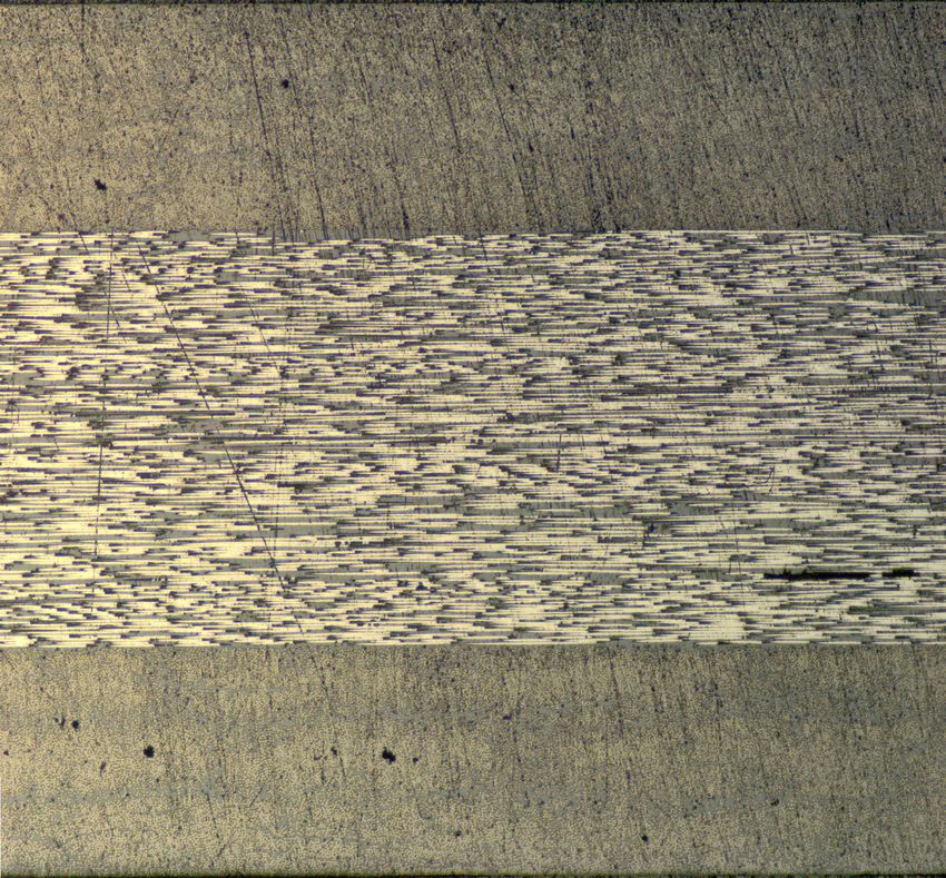
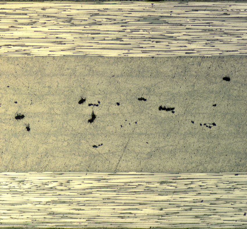
(a) Plate 1, K5, 90deg (2-1F) (b) Plate 2, K5, 0deg (2-2D)
Figure 6: Comparison of micrographs with different noise amounts with their
respective Table 5 labels. a) Low noise. b) High noise.
3.3 Void content computation methods
The computation of void content was performed using three methods: selection, thresh-
olding, and machine learning. The details are described in the following sections, with
instructions to the methods described in Appendix B.
3.3.1 Selection-method
The selection-method uses edge detection selection tools to compute void content. This
is done by manually selecting each void and count the area fraction of the void selection
over the entire image using a histogram, resulting in the void content for that image.
Manually tracing a void’s edge would be extremely tedious, but with edge detection
tools it usually only requires one mouse click inside the void area and the edge is im-
mediately selected.
Programs that include edge detection selection tools and histograms are raster graphics
editors, such as Adobe® Photoshop® version CS3 and on, or Affinity® Photo version
1.5 and on. Adobe calls this tool the “Quick Selection tool” while Affinity calls it the
“Selection brush tool”. The way edge detection tools can find an edge is by applying
edge detection algorithms on the selected pixels. These algorithms then analyze the
14differences in these and the surrounding pixels, usually searching for rapid changes in
intensity and brightness. This advantageously also means that the selection tool will
select the same edges regardless of user or if the pixels were deselected for example,
increasing repeatability and reproducibility between users. Examples of edge detectors
include Sobel, Prewitt, and Canny edge detectors [45]. As an example, a palm tree has
been separated from its background with the use of an edge detection selection tool in
Figure 7.
(a) (b)
Figure 7: Example showing the ability of edge detection selection tools in find-
ing and selecting detailed edges. Here, edges of a palm tree has been selected
and separated from its background.
3.3.2 Thresholding
Thresholding is the simplest method of image segmentation. The method is based on
selecting a level, or “threshold”, of brightness where all pixels in the image with higher
brightness become white/black and all other pixels become black/white, resulting in a
binary segmented image. Thresholding has a special function in void content computa-
tion due to voids always being black in color and explicitly darker than its surroundings,
resulting in an easier segmentation. A simple segmentation process is shown in Figure 8
with Figure 9 showing its corresponding histogram and threshold level. In a histogram,
the x-axis represents the intensity values of the pixels, 0 being an entirely black pixel
and 255 being an entirely white pixel, and the y-axis represents the number of pixels
with each intensity. The reason the values are 0-255 is because it is an 8-bit image
able to contain 256 (28 ) different colors. Due to the voids, a small peak is found in the
left-most side in the histogram in Figure 9a, but all the void pixels do not lie within this
peak due to some having a lighter hue.
15(a) (b) (c)
Figure 8: Sequence of images showing the process of thresholding. a) Original
image greyscaled. b) Selecting the threshold level where voids are separated
from background. c) Thresholded binary image.
(a) (b)
Figure 9: Corresponding histogram and threshold level for Figure 8. a) His-
togram. b) Thresholding using histogram.
Programs that can threshold images include raster graphics editors and image process-
ing programs, the latter being the most prominently used for this purpose. Fiji is an
open-source free image processing program recommended for this use. It has the ability
to provide analysis on the thresholded voids, such as the area fraction. Unfortunately
for scientific purposes, Fiji does provide the area fraction directly while thresholding,
as can be seen below the histogram in Figure 9b. This means that the user can directly
choose the void area fraction which is a clear bias.
In order to save time and effort, a macro was written in ImageJ Macro Language (IJM)
which automates the repeatable processes in the thresholding method, such as opening
an image, greyscaling it and saving the results. The macro lets the user choose the file
directory for the images, opens up the first image inside the directory and lets the user
16choose a threshold and optionally a noise filter, after which the macro saves the void
area fraction to a table and repeats the process for the next image in the directory. This
macro is available in Appendix C.
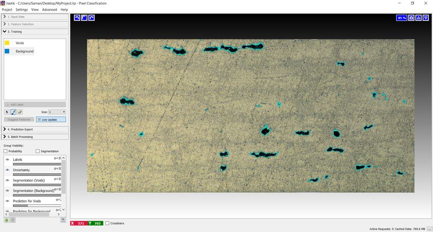
3.3.3 Machine learning-method
The machine learning-method is based on teaching a program to segment void areas
automatically by labelling parts of some training images as “voids” and “background”.
The machine learning program will then apply filters and algorithms on the image
and make qualified guesses on which label each pixel throughout the image belongs
to. Each pixel receives a probability on what label they belong to and pixels with
ambiguous results have higher uncertainty. The method is then used to classify pixels
in new images the program is unfamiliar with. This is called pixel classification.
An important element of machine learning is to reduce the uncertainty about its
classifications.
Ilastik is a free open-source machine learning program suitable for pixel classification.
Ilastik applies filters to the training images to find features inside the image. These
filters search for features including edges, color/intensity, and textures and can be
applied in different strength levels, called “sigma”-levels. The sigma-level refers to the
strength of the Gaussian smoothing applied on the image before applying the filter.
Figure 10 shows three different sigma-levels applied on a micrograph. Note how lower
sigma-levels fit to smaller details and how higher sigma-levels find the rougher outlines.
Higher sigma-levels can thus attain information about the larger neighborhoods while
smoothing out the finer details.
Figure 10: Different Gaussian filter strengths (sigma) applied to a micrograph
shows how different sigma-levels can extract information on different levels of
detail.
Once the filters are applied, the user labels pixels in the image and a pixel classifier
trains itself on these labelled pixels. Many different pixel classifier algorithms are avail-
able in ilastik, the default one being a “Random Forest” classifier which uses large
groups of decision trees to find a class for each pixel. When the training images have
been labelled and satisfyingly segmented by the machine learning program, the images
17can be exported and most importantly, batch processing can be applied. Batch pro-
cessing can apply the trained program to a large batch of images and process them at
once. The pixels in the exported images will have values corresponding to the label
number they belonged to. In other words, label number 1 will have pixel intensity 1
etc., making the exported image look entirely black. Next, the void area fraction of the
exported image has to be calculated. Since the exported image only has two labels, e.g.
“voids” and “background”, this can be done with thresholding. A macro was written in
Fiji automating the process of opening, thresholding, finding the void area fraction of
an image and saving the results in a table for a set of images, enabling the entire batch
of exported images to be analyzed altogether. This macro is available in Appendix D.
3.4 Multiple-user trials
The three void content computation methods were performed on the produced micro-
graphs by three users with academic backgrounds, experienced in digital image anal-
ysis, one of whom being the author. All three users followed the instructions for the
three methods described in Appendix B, to ensure the same procedures were carried
out by all users. The obtained void content results were then compared between users
and between methods. The aim was to find a method able to produce similar results
even between different users, able to produce consistent results on the same image for
different tries, and a method quick and simple to learn.
3.4.1 Trial 1
The first trial consisted of computing void content on 10 randomly selected images
from all three plates using the three methods. The void content for each image was
then compared between the users through population standard deviation. This stan-
dard deviation was used to compare the performance of the three methods in attaining
similar results between different users. Four of these images were used to train the
machine learning program.
3.4.2 Trial 2
The second trial consisted of computing void content using the three methods on the
three plates containing 12 images each. Aside from calculating the void contents for
each image, the total void content for each plate was calculated. The standard devia-
tions for the images were compared between users and methods. Six images from Plate
1 were used to train the machine learning program. All images were taken from Plate
1 to simulate the realistic use of the method where the program would be unfamiliar
with images from future specimens.
184 Results
4.1 Trial 1
A box diagram of the standard deviations between the three users void contents for
the three methods is shown in Figure 11. Population standard deviation was applied,
described in Equation 5 where σ is the population standard deviation, µ the population
mean value, n the number of data points, and x a data point in the set. The data
points in the diagram consists of the standard deviations between the three users void
content results on each of the 10 images. In contrast, Figure 12 compares the standard
deviations of each user between the three methods they used, revealing performance
differences in attaining consistent void content results when using different methods.
All resulting data points for trial 1 are specified in Table 4 in Appendix A.
s
Pn
i=1 |x − µ|2
σ= (5)
n
0.6%
0.55%
0.5%
0.45%
0.4%
Standard deviation
0.35%
0.3%
0.25%
0.2%
0.15%
0.1%
0.05%
0%
Selection-method Thresholding Machine Learning-
method
Figure 11: Standard deviation of each method’s results between the three users
in trial 1. The data points in each box chart consists of the standard deviation
between the three users void content results on each of the 10 images.
190.6%
0.55%
0.5%
0.45%
0.4%
Standard deviation
0.35%
0.3%
0.25%
0.2%
0.15%
0.1%
0.05%
0%
User 1 User 2 User 3
Figure 12: Standard deviation of each user’s results between the three methods
in trial 1. The data points in each box chart consists of the standard deviation
between the methods’ void content results on each of the 10 images.
4.2 Trial 2
Likewise for trial 2, Figure 13 shows a box diagram for the standard deviation of the
void contents for the three methods. Equivalently, the data points here consists of the
standard deviations between the three users void content results, but this time for the
12 images for each plate. Figure 14a shows the standard deviation between the meth-
ods for each user. In this diagram, each bar represents the standard deviation between
the total plate void content calculated by the three methods. Figure 14b shows the same
diagram but has the standard deviation normalized with each plate’s total void content
since the plates contain different void content levels. Additionally, Figure 15 shows the
Z-score, or standard score, for each of the three methods total plate void contents cate-
gorized by user. The Z-score is a measurement of how many standard deviations away
each data point is from the mean. In this case, there are three total plate void contents
obtained for each plate, one from each method. The mean value of these are taken and
the Z-score shows which method has the most deviating result from this mean. The Z-
score is useful since it does not show the standard deviation, but the number of standard
deviations away from the mean, which normalizes differences between the plates since
they do not have exactly the same void contents and standard deviations. Equation 6
describes the Z-score formula, where Z represents the Z-score, µ the population mean
20value, and σ the population standard deviation. The diagram is categorized by user to
reveal potential similarities or dissimilarities between the deviations for different users.
All resulting data points for trial 2 are specified in Table 5 and Table 6 in Appendix A.
|x − µ|
Z= (6)
σ
0.5%
0.45%
0.4%
0.35%
Standard deviation
0.3%
0.25%
0.2%
0.15%
0.1%
0.05%
0%
Selection-method Thresholding Machine Learning-
method
Plate 1 Plate 2 Plate 3
Figure 13: Standard deviation of each method’s results between the three users
in trial 2. The data points in each box chart consists of the standard deviation
between the three users void content results on each of the 12 images in each
plate.
210.15%
Standard deviation
25%
standard deviation
Normalized
20%
0.1%
15%
10%
0.05%
5%
User 1 User 2 User 3 User 1 User 2 User 3
Plate 1 Plate 2 Plate 3 Plate 1 Plate 2 Plate 3
(a) (b)
Figure 14: a) Standard deviation between the methods for each user in trial
2. Each bar represents the standard deviation between the total plate void
content calculated by the three methods. b) Normalized standard deviation
between the methods for each user in trial 2, normalized for each plate’s total
void content. Each bar represents the fraction of the total plate void content
the standard deviation consisted of.
140%
120%
100%
Z-score
80%
60%
40%
20%
User 1 User 2 User 3
Selection-method
Thresholding
Machine Learning-method
Figure 15: Z-score for the methods’ total plate void contents categorized by
user in trial 2. The Z-score is a measurement of how many standard deviations
away each data point is from the mean.
22You can also read